ANALYSIS OF DIFFUSION PROBLEMS USING HOMOTOPY PERTURBATION AND VARIATIONAL ITERATION METHODS

ANALYSIS OF DIFFUSION PROBLEMS USING HOMOTOPY

PERTURBATION AND VARIATIONAL ITERATION METHODS

A. Barari1*, A. Tahmasebi Poor2, A. Jorjani3& H. Mirgolbabaei4

1

Department of Civil Engineering, Aalborg University, Sohngårdsholmsvej 57, 9000 Aalborg, Aalborg 2

Khazar Ab Consulting Engineers Corporation, Sari, Mazandaran, Iran 3

Department of Civil Engineering, University of Mazandaran, Babol, Iran 4

School of Mechanic, Islamic Azad University, Jouybar Branch, Jouybar, Iran

ABSTRACT

In this paper, variational iteration method and homotopy perturbation method are applied to different forms of diffusion equation. The diffusion equations have found wide applications in heat transfer problems, theory of consolidation and many other problems in engineering. The methods proposed to solve the diffusion equations herein have been applied to a variety of problems in the recent past, and have proved to yield highly accurate solutions. Comparison is made between the exact solutions and the results of the variational iteration method (VIM) and homotopy perturbation method (HPM) in order to verify the accuracy of the results, revealing the fact that these methods are very effective and simple.

Keywords: homotopy perturbation method (HPM); variational iteration method (VIM); diffusion equation; exact solution

1. INTRODUCTION

Diffusion equations have important applications in various fields of applied mathematics. In soil mechanics applications, Terzaghi [1] showed that the theory of one dimensional consolidation is governed by the diffusion equation. Many other applications have been

mentioned in the literature for different variations of the diffusion equation [2-4]. It is of prime importance therefore, to develop effective solution procedures for this equation.

Aside from analytical solutions, finite difference methods have been traditionally used to solve the diffusion equation. In this paper, the variational iteration method (VIM) [5-9] and the homotopy perturbation method (HPM) [10-14] have been successfully applied to solve the diffusion equations. These methods were introduced to overcome the shortcomings of the conventional perturbation methods, which are dependent on assuming small parameters and therefore the results are valid only for small values of the small parameter chosen. Specifically, the VIM provides the solution (or an approximation to it) to ordinary and partial differential equations as a sequence of iterates and does not require that the nonlinearities be differentiable with respect to the dependent variable and its derivatives. The merits of this method make it attractive for application to problems in different fields of applied mathematics.

In the following sections, an overview of VIM and HPM is presented, followed by the application of these methods to both linear and nonlinear forms of the diffusion equation.

2. BASIC IDEA OF HOMOTOPY-PERTURBATION METHOD

To explain this method, let us consider the following function:

A u

( )



f r

( )



0,

r

 

(1)

with the boundary conditions of:

B u

( ,

u

)

0,

r

,

n





 



(2)

where

A

,

B

,

f r

( )

and



are a general differential operator, a boundary operator, a known analytical function and the boundary of the domain



, respectively.

L u

( )



N u

( )



f r

( )



0,

(3) By the homotopy technique, we construct a Homotopy

v r p

( , ) :

 

[0,1]



R

which satisfies

( , )

(1

)

( )

(

0

)



( )

( )



0,

[0,1],

,

H v p

p

L v

L u

p A v

f r

p

r

 











 









₍₄₎

or

H v p

( , )



L v

( )



L u

(

₀

)



pL u

(

₀

)



p N v



( )



f r

( )





0,

(5)

where

p



[0,1]

is an embedding parameter, while

u

₀ is an initial approximation of Eq. (1), which satisfies the boundary conditions. Obviously, from Eqs. (4) and (5) we will have:

H v

( , 0)



L v

( )



L u

(

₀

)



0,

(6)

H v

( ,1)



A v

( )



f r

( )



0,

(7)

The changing process of p from zero to unity is just that of

v r p

( , )

from

u

₀ to

u r

( )

.In topology, this is called deformation, while

( )

(

)

0

L v



L u

and

A v

( )



f r

( )

are called homotopy.

According to the HPM, we can first use the embedding parameter p as a “small parameter”, and assume that the solutions of Eqs. (4) and (5) can be written as a power series in p:

2

...,

0

1

2

v



v



pv



p v



(8)

Setting

p



1

yields in the approximate solution of Eq. (8) to:

lim

₀

₁

₂

,

1

u

v

v

v

v

p





 







(9)

The combination of the perturbation method and the homotopy method is called the HPM, which eliminates the drawbacks of the traditional perturbation methods while keeping all its advantage.

The series (9) is convergent for most cases. However, the convergent rate depends on the nonlinear operator

A v

( )

. Moreover, He [10] made the following suggestions:

 The second derivative of

N v

( )

with respect to v must be small because the parameter may be relatively large, i.e.

p



1

.

 The norm of 1 N

L v

 

 must be smaller than one so that the series converges.

3. BASIC IDEA OF VARIATIONAL ITERATION METHOD

To clarify the basic ideas of VIM, we consider the following differential equation:

( ),

Lu



Nu



g t

(10)

where

L

is a linear operator,

N

is a nonlinear operator and

g

(t

)

is a homogeneous term. According to VIM, we can write down a correction functional as follows:

 



 



_



 



   







t

n n

n

n

t

u

t

Lu

N

u

g

d

u

0 1

~

_

_

_





(11)

where



is a general lagrangian multiplier which can be identified optimally via the variational theory. The subscript n indicates the nthapproximation and

u

_n is considered as a restricted variation, i.e.



u

~

_n



0

.

4. NUMERICAL ILLUSTRATIONS:

Example 1: First, consider the simple form of the equation [15]:

2 2

( , )

( , ) , 0

1, 0

1

u x t

u x t

x

t

t

x



_



_{ }

_{ }





(12)

While in reality the value of x and t would vary between [0, l] and [0, t], the range [0, 1] given in Eq. (12) indicates a normalization of the variables relative to their maximum value. The exact solution along with the initial and boundary conditions of Eq. (12) are known to be:

2

( )

( , )

t

sin(

), 0

1, 0

1

U x t



e





x

 

x

 

t

(13)

To solve Eq. (12) by means of HPM, we consider the following process after separating the linear and nonlinear parts of the equation. A homotopy can be constructed as follows:

2

0 2

( , ) (1 ) (

( , )

( , )

( , )

( , ) ,

H v p p p

t

v x t

t

v x t

t

v x t

x

v x t

   

  

   







_



_

















(14)

Substituting

v



v

₀



pv

₁



...

in to Eq. (14) and rearranging the resultant equation based on powers of p-terms, it can be written:

with the following conditions:

0( , 0) sin

( , 0) 0

1, 2,...

i

v x x

v x

i

 





(18)

The effective initial approximation for

v

₀ may be obtained from the conditions stated in Eq. (18) and therefore solutions of Eqs. (15-17) may be written as follows:

v

₀

( , )

x t



sin(



x

)

(19)

2

1

( , )

sin(

)

v x t

 

 

x

t

(20)

4 2

2

( , )

1

sin(

)

2

v

x t



 

x

t

(21)

In the same manner, the rest of components were obtained using the Maple package. According to the HPM, we can conclude that:

( , )

lim ( , )

0

( , )

1

( , ) ... ,

1

u x t

v x t

v x t

v x t

p











(22)

Therefore, substituting the values of

v x t

₀

( , )

,

v x t

₁

( , ),

v x t

₂

( , )

from Eqs. (19-21) in to Eq. (22) yields:

2 4 2

( , )

sin(

) sin(

)

1

sin(

)

2

u x t





x



 

x

t



 

x

t

(23)

Further manipulation of Eq. (23) will give:

2 4 2

( , )

sin(

)(1

1

)

2

u x t





x





t





t

(24)

p

0

:

v x t

₀

( , )

0,

t







(15)

2 1

1 2 0

:

( , )

( , )

0,

p

v x t

v x t

t

x



_



_





(16)

2 2

1 2 0

:

( , )

( , )

0,

p

v x t

v x t

t

x



_



_

It should be noted that Eq. (24) is the result of only three terms calculated from Eqs. (15-17). If further calculation of higher powers of pwere to be derived, then it would be clear that the second part on the right hand side of Eq. (24) i.e (1 2 1 4 2)

2

t t





  is the expansion of series e



2tand therefore Eq. (24) will take the following form:

u x t

( , )



sin(



x

)

e

2t (25)

which is the exact solution of Eq. (12).

Now, we will show that Eq. (12) may be effectively solved by means of the VIM to reach the same exact solution. In order to do so, one can construct the following correction functional,

2

2 0

( , )

( , )

1

( , )

( , )

t

n n

u

x t

u

_n

x t

n

u

x

u

x

d

x





















_







_

_









(26)

Stationary conditions for Eq. (26) can be obtained as follows:

0,

1

0,

t

t

 

















(27)

We obtain the lagrangian multiplier:



 

1

(28)

As a result, we obtain the following iteration formula:

2

2 0

( , )

( , )

1

( , )

( , )

t

n n

u

x t

u

_n

x t

n

u

x

u

x

d

x

























_



_











(29)

The above formulation needs to start with an initial approximation which satisfies the initial conditions. Obviously, in this case the initial approximation may be obtained from the initial condition of the problem, i.e.

u x t

0

( , )



sin(



x

)

(30)

Using the above variational formula (29) and substituting the initial approximation from Eq. (30), it can be written:

1

2 2 0

( , )

sin(

)

sin(

)

sin(

)

t

u x t

x

x

x

d

x

















_



_







_

_









(31)

The rest of the components of the iteration formula can be obtained, each time by replacing the approximation from the previous iteration into the new iteration formula. Solving Eq. (31),u1(x,t) will be obtained as:

2

1

( , )

sin(

)( 1

)

u x t

 



x

 



t

(32)

The second iteration can then be obtained following the same procedure. Therefore,

2 2

2

2 2

2 0

( , )

sin(

) ( 1

)

( sin(

) ( 1

))

( sin(

) ( 1

))

t

u x t

x

t

x

x

d

x







 



 





 

 





_



_

_{ }

_



_

_{ }





_

_









(33)

2 4 2 2

1

( , )

sin(

)(2 2

)

2

u x t





x





t





t

(34)

It can be seen that if further iterations are added to the above calculations, the second part of the right hand side of Eq. (34) will form the series expansion of e



2t. Therefore once again the exact solution of the diffusion problem is achieved through the VIM. Figure (1) shows variation of u(x,t) for several values of tobtained from solution of VIM and HPM for Eq.(12). Furthermore, three dimensional comparison of exact solution and results of HPM and VIM are plotted in Figure (2) which reveals the high agreement between the results.

Fig 1.Results of VIM, HPM and exact solution for Eq.(12)

Fig 2.Results of exact solution, VIM and HPM for Eq. (12)

Example 2:The second example used to illustrate the ability of the HPM and VIM in solving diffusion equations involves a nonlinear term. Consider the following diffusion equation with a nonlinear reaction term [16]:

2

2 3

2

( , )

( , )

( , )

( , ) , 0

10,

0

u x t

u x t

u x t

u x t

x

t

t

x



_



_

_

_{ }

_





(35)

With the initial and boundary conditions taken from the exact solution given by [16]:

( )

1

1

( , )

,

1

x t

2

u x t

e

 









(36)

To solve Eq. (35) by means of HPM, we consider the following process after separating the linear and nonlinear parts of the equation. A homotopy can be constructed as follows:

0 2

2 3

2

( , )

(1

) (

( , )

( , )

( , )

( , )

( , )

( , )

,

H v p

p

t

t

p

t

v x t

v x t

v x t

v x t

v x t

v x t

x





 



























_



_

_





_







(37)

p

0

:

v x t

₀

( , )

0,

t







(38) 2

1 2 3

0 2 0 1 0

:

( , )

( , )

( , )

( , )

0,

p

v x t

v x t

v x t

v x t

x

t



















(39)

2

2 2

1 0 1 0 1 2

2

: (

( , )) 3 ( , )

( , ) 2 ( , ) ( , ) (

( , ))

0,

p

v x t

v x t v x t

v x t v x t

v x t

x

t



















(40)

With the following conditions:

(0.7071 ) 1 ( , 0)

0 ₁

( , 0) 0

1, 2,...

x x e x i

v

v

i

  



(41)

With the effective initial approximation for

v

₀ from the conditions (41) and solutions of Eqs. (38-40) may be written as follows:

₀

( , )

1

_{(0.7 )}

,

1

x

v x t

e





(42) 7 7 ( ) ( ) 10 10 1 7 ( ) 3 10

( , )

49

51

,

100(1

)

x x x

v x t

te

e

e



















(43) 7 7 ( ) ( )

7 10 5

( ) 2 ₁₀

21 ( )

10

2 _{7 7 21 14 7}

( ) ( ) ( ) ( ) ( )

4 _{10 5 10 5 2}

( , )

2589

2989

2601 2401

,

2 10

1 5

10

10

5

x x

x

x

x x x x x

v x t

e

e

t e

e

e

e

e

e

e

 





































_

_





































_

_







(44)

In the same manner, the rest of components were obtained using the Maple package. According to the HPM, we can conclude that:

u x t

( , )



lim ( , )

v x t



v

₀

( , )

x t



v x t

₁

( , ) ... ,



p



1

(45)

Therefore, substituting the values of

v x t

₀

( , )

,

v x t

₁

( , ),

v x t

₂

( , )

from Eqs. (42-44) in to Eq. (45) yields:

7 7 ( ) ( ) 10 10 7 (0.7 )

( ) ₃ 10

7 7

( ) ( )

7 10 5

( ) 2 ₁₀

21 ( )

10

7 7 21 14 7

( ) ( ) ( ) ( ) ( )

4 10 5 10 5 2

( , )

49 51

1 1

100(1 )

2589 2989 2601 2401

,

2 10 1 5 10 10 5

x x x x x x x x

x x x x x

u x t

te e e e e e t e e

e e e e e

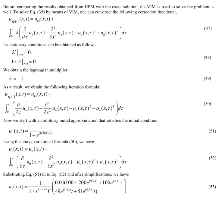
Before comparing the results obtained from HPM with the exact solution, the VIM is used to solve the problem as well. To solve Eq. (35) by means of VIM, one can construct the following correction functional,

2

2 3

2 0

( , )

( , )

1

( , )

( , )

( , )

( , )

t

n n n n

u

x t

u

_n

x t

n

u x

u x

u x

u x

d

x





































_

_









(47)

Its stationary conditions can be obtained as follows:

0,

1

0,

t

t

 

















(48)

We obtain the lagrangian multiplier:

1



 

(49)

As a result, we obtain the following iteration formula:

2

2 3

2 0

( , )

( , )

1

( , )

( , )

( , )

( , )

t

n n n n

u

x t

u

_n

x t

n

u x

u x

u x

u x

d

x























_



_

_





_

_









(50)

Now we start with an arbitrary initial approximation that satisfies the initial condition:

0 (0.7071 )

1

( , )

1

x

u x t

e





(51)

Using the above variational formula (50), we have:

1 0

2

2 3

0 2 0 0 0

0

( , )

( , )

( , )

( , )

( , )

( , )

t

u x t

u x t

u x

u x

u x

u x

d

x

































_

_









(52)

Substituting Eq. (51) in to Eq. (52) and after simplifications, we have: (0.7 ) 1.4 1 (0.7 ) 3 (1.4 ) (0.7 )

0.01(100 200

100

1

( , )

1

)

49

51

)

x x

x x x

e

e

u x t

e

e

t

e

t















_



_



_



_

(53)

and so on. In the same way the rest of the components of the iteration formula can be obtained. The comparison of the results is illustrated in Figs. (3) and (4).

5. CONCLUSIONS

Homotopy perturbation method and variational iteration method are employed successfully to study two different forms of diffusion equation. In conclusion, HPM and VIM provide highly accurate numerical solutions for linear and nonlinear problems. As it is mentioned, these methods avoids linearization and physically unrealistic assumptions. Finally, Comparison with exact solution reveals that homotopy perturbation method and variational iteration method are remarkably effective for solving nonlinear problems.

REFERENCES

[1] Terzaghi, K. (1943). Theoretical Soil Mechanics. John wiley, New York.

[2] Seed, H. B., Philippe, P. M. and Lysmer, J. (1975). The Generation and Dissipation of Pore Water Pressures During Soil Liquefaction. Report, EERC-75-26, 27p.

[3] Pironneau, O. (1982). On The Transport-Diffusion Algorithm and its Applications to The Navier–Stokes Equations.Numerische Mathematik, 38, 309–332.

[4] Li,W. (2000). Mixed Finite Analysis Methods for Viscous Fluids. China Science Press, Beijing.

[5] He, J. H. (1999). Variational Iteration Method: A Kind of Nonlinear analytical technique: some examples.

Internat.J. Nonl. Mech, 34, 699–708.

[6] He, J. H. (2000).Variational Iteration Method for Autonomous Ordinary Differential Systems. Appl. Math. Comput,114, 115–123.

[7] Ganji, D. D. and Sadighi, A. (2007). Application of Homotopy–Perturbation and Variational Iteration Methods to Nonlinear Heat Transfer and Porous Media Equations. J. Comput. Appl. Math, 207, 24-34.

[8] Ganji, D.D., Jannatabadi, M. and Mohseni, E. (2007). Application of He’s Variational Iteration method to nonlinear Jaulent–Miodek equations and comparing it with ADM.

J. Comput. Appl. Math, 207, 35-45.

[9] Rostamian, M., Barari, A. and Ganji, D.D. (2008). Application of Variational Iteration Method to Dissipative Wave Equation, J. Phys, 96, 1-5.

[10] He, J. H. (1999). Homotopy Perturbation Technique. Comput Methods Appl. Mech. Eng,178, 257–262.

[11] He J. H., (2006). New Interpretation of Homotopy Perturbation Method. Int. J. Mod. Phys. B,20,2561–2568.

[12] Rafei, M. and Ganji, D.D. (2006). Explicit Solutions of Helmholtz Equation and Fifth–order Kdv Equation using Homotopy–perturbation Method.Int. J. Nonlinear Sci. Numer. Simul,7,321–328 .

[13] Ganji, D.D., Sadighi, A. (2006). Application of He’s Homotopy–Perturbation Method to Nonlinear Coupled Systems of Reaction–diffusion Equations, Int. J. Nonlinear Sci. and Num. Simu, 7,411–418.

[14] Barari, A., Omidvar, M., Gholitabar, S. and Ganji, D. D. (2007). Variational Iteration Method and Homotopy-Perturbation Method for Solving Second-Order Non-Linear Wave Equation, AIP Conference Proceedings,

936, 81-85.

[15] Sulaiman, J., Othman, M. and Hasan, M. K. (2004). Quarter-sweep Iterative alternating decomposition explicit algorithm applied to diffusion equations, International Journal of Computer Mathematics, 81, 1559 – 1565. [16] Chawla, M. M. and Evans, D. J. (2005). A new L-stable Simpson-type rule for the diffusion equation,