Recent developments of some asymptotic methods and their
applications for nonlinear vibration equations in engineering
problems:A review
Abstract
This review features a survey of some recent developments in asymptotic techniques and new developments, which are valid not only for weakly nonlinear equations, but also for strongly ones. Further, the achieved approximate analytical solutions are valid for the whole solution domain. The lim-itations of traditional perturbation methods are illustrated, various modified perturbation techniques are proposed, and some mathematical tools such as variational theory, homo-topy technology, and iteration technique are introduced to over-come the shortcomings.In this review we have applied different powerful analytical methods to solve high nonlin-ear problems in engineering vibrations. Some patterns are given to illustrate the effectiveness and convenience of the methodologies.
Keywords
Nonlinear Vibration; Nonlinear Response; Analytical Meth-ods ;Parameter Perturbation Method (PPM) ; Variational Iteration Method(VIM);Homotopy Perturbation Method (HPM); Iteration Perturbation Method (IPM); Energy Bal-ance Method (EBM); Parameter-Expansion Method (PEM) ; Variational Approach (VA);Improved Amplitude Frequency Formulation (IAFF);Max-Min Approach (MMA); Hamilto-nian Approach (HA); Homotopy Analysis Method (HAM); Review
Mahmoud Bayat∗a,Iman Pakara and Ganji Domairryb
a
Department of Civil Engineering, Mashhad Branch, Islamic Azad University, Mashhad, Iran
Tel/Fax : (+98 111 3234205)
b
Department of Mechanical Engineering, Babol University of Technology, Babol, Iran
Received 02 Feb 2011; In revised form 22 May 2012
∗Author email: mbayat14@yahoo.com
1
Contents 2
1 INTRODUCTION 3
3
2 Parameterized Perturbation Method (PPM) 3
4
2.1 Basic idea of Parameterized Perturbation Method . . . 4
5
2.2 Application of Parameterized Perturbation Method . . . 4
3 Variational Iteration Method (VIM) 7 7
3.1 Basic idea of Variational Iteration Method . . . 7
8
3.2 Application of Variational Iteration Method . . . 8
9
4 Homotopy Perturbation Method (HPM) 14
10
4.1 Basic idea of Homotopy Perturbation Method . . . 14
11
4.2 Application of Homotopy Perturbation Method . . . 15
12
5 Iteration Perturbation Method (IPM) 21
13
5.1 Basic idea of Iteration Perturbation Method . . . 21
14
5.2 Application of Iteration Perturbation Method . . . 22
15
6 Energy Balance Method (EBM) 26
16
6.1 Basic idea of Energy Balance Method . . . 27
17
6.2 Application of Energy Balance Method . . . 28
18
7 Parameter –Expansion Method (PEM) 37
19
7.1 Basic idea of Parameter–Expansion Method . . . 38
20
7.2 Application of Parameter –Expansion Method . . . 39
21
8 Variational Approach (VA) 42
22
8.1 Basic idea of Variational Approach . . . 42
23
8.2 Application of Variational Approach . . . 43
24
9 Improved Amplitude-Frequency Formulation (IAFF) 51 25
9.1 Basic idea of Improved Amplitude-Frequency Formulation . . . 51
26
9.2 Application of Improved Amplitude-Frequency Formulation . . . 52
27
10 Max-Min Approach (MMA) 62
28
10.1 Basic idea of Max-Min Approach . . . 63
29
10.2 Application of Max-Min Approach . . . 64
30
11 Hamiltonian Approach (HA) 76
31
11.1 Basic idea of Hamiltonian Approach . . . 76
32
11.2 Application of Hamiltonian Approach . . . 77
33
12 Homotopy Analysis Method (HAM) 80
34
12.1 Basic idea of Homotopy Analysis Method . . . 80
35
12.2 Application of Homotopy Analysis Method . . . 82
36
13 Conclusions 83
1 INTRODUCTION 38
Most of engineering problems, especially some oscillation equations are nonlinear, and in most
39
cases it is difficult to solve such equations, especially analytically. Recently, nonlinear oscillator
40
models have been widely considered in physics and engineering. It is obvious that there are
41
many nonlinear equations in the study of different branches of science which do not have
42
analytical solutions. Due to the limitation of existing exact solutions, many analytical and
43
numerical approaches have been investigated. Therefore, these nonlinear equations must be
44
solved using other methods. Many researchers have been working on various analytical methods
45
for solving nonlinear oscillation systems in the last decades. Perturbation technique is one the
46
well- known methods [3, 11, 34, 37, 39, 85], the traditional perturbation method contains
47
many shortcomings. They are not useful for strongly nonlinear equations, so for overcoming
48
the shortcomings, many new techniques have been appeared in open literatures.
49
It should be mentioned that several books appeared on the subject of mathematical
meth-50
ods in engineering problem during the past decade [10, 48, 54, 77, 113, 125, 133, 137, 144–
51
146, 180, 186, 187].
52
The aim of this article is to review the recent research on the approximate analytical
53
methods for nonlinear vibrations. The applications of these methods have been appeared in
54
open literatures in the last three years. There are hundreds of published papers too numerous to
55
refer to all of them, but for the purpose of filling the gaps in the present summary, Refs[14, 15,
56
28, 30, 36, 40, 47, 55, 66, 75, 76, 83, 88, 89, 94, 142, 166, 170, 173, 178, 192, 193, 210, 217]may
57
offer good help in overcoming the inevitable shortcomings in a condensed presentation. To
58
show the efficiency and accuracy of the methods some comparisons have done with the results
59
obtained by those methods and numerical methods and they are valid for whole domain. Some
60
of the ideas first appeared in this review article, and most cited references were published in
61
the last three years, revealing the most emerging research fronts. In this review, the basic
62
idea of each method is presented then some examples are illustrated and discussed to show the
63
application of these methods.
64
2 PARAMETERIZED PERTURBATION METHOD (PPM) 65
Recently, nonlinear oscillator models have been widely considered in physics and engineering.
66
Study of nonlinear problems which are arisen in many areas of physics and also engineering
67
is very significant for scientists. Surveys of the literature with numerous references have been
68
given by many authors utilizing various analytical methods for solving nonlinear oscillation
69
systems. Non-linear problems continue to be as a challenge, and heed has mainly concentrated
70
on qualitative changes of systems bifurcations and instability. Parameterized Perturbation
71
Method (PPM) is one of the well-known methods for solving nonlinear vibration equations.
72
The method was proposed in by He in 1999 [80].It was rarely used recently, but this method is
73
a kind of powerful tool for treating weakly nonlinear problems, but they are less effective for
74
analyzing strongly nonlinear problems [37, 50, 86, 92, 115, 160].
2.1 Basic idea of Parameterized Perturbation Method 76
For the nonlinear equation L(u)+N(u)=0, whereL and N are general linear and nonlinear
77
differential operators respectively, a linear transformation can be introduced as:
78
u=εν (2.1)
We can assume that ν can be written as a power series inε,as following
79
ν=ν0+εν1+ε2ν2+..., (2.2)
And
80
ν=lim ε→1ν
=ν0+ν1+ν2+ν3+... (2.3)
2.2 Application of Parameterized Perturbation Method 81
Two examples have considered showing the applicability of this method.
82
83
Example 1 84
Consider the following Duffing equation:
85
¨
u+αu+βu3=0, u(0)=A, u˙(0)=0 (2.4)
We let u=εν in Eq. (2.4) and obtain
86
¨
ν+αν+ε2βν3=0, ν(0)=A/ε , ν˙(0)=0 (2.5)
Supposing that the solution of Eq. (2.5)and ω2can be expressed in the form
87
ν=ν0+ε2ν1+ε4ν2+ε6ν3 (2.6)
α=ω2+ε2ω1+ε4ω2+ε6ω3 (2.7)
Substituting Eqs. (2.6) and (2.7) into Eq. (2.5) and equating coefficients of like powers of
88
εyields the following equations
89
¨
ν0+ω2ν0=0, ν0(0)=A/ε , ν˙0(0)=0, (2.8)
90
¨
ν1+ω2ν1+ω1ν0+βν03=0, ν1(0)=0,ν˙1(0)=0 (2.9)
Solving Eq. (2.8) results in
91
ν0=
A
ε cosω t (2.10)
Equation (2.9), therefore, can be re-written down as
¨
ν1+ω2ν1+(ω1+ 3βA2
4ε2 )
A
ε cos(ω t)+ βA3
4ε3 cos(3ω t)=0. (2.11)
Avoiding the presence of a secular terms needs:
93
ω1=−
3βA2
4ε2 (2.12)
Substituting Eq. (2.12) into Eq. (2.7)
94
ωP P M = √
α+3
4βA
2 (2.13)
Solving Eq. (2.11), gives:
95
ν1=−
A3β
32ω2ε3(cos(ω t)−cos(3ω t)) (2.14)
Its first-order approximation is sufficient, and then we have:
96
u=εν=ε(ν0+ε2ν1)=Acos(ω t)−
A3β
32ω2ε3[cos(ω t)−cos(3ω t)] (2.15)
The exact frequency of this problem is:
97
ωExact=2π/4 √
2∫ π/
2
0
dt
√
βA2cos2(t)+βA2+2α (2.16)
Table 2.1 Comparison of the approximate frequencies with the exact period.
A α β Present Study Exact Error %
(PPM) Solution (ωP P M−ωex) /ωex
0.1 0.5 0.1 0.7076 0.7076 0.0000
0.5 0.1 2 0.6892 0.6800 1.3501
1 2 0.5 1.5411 1.5403 0.0520
2 5 2 3.3166 3.2958 0.6313
5 2 5 9.7852 9.5818 2.1228
10 1 0.5 6.2048 6.0772 2.0994
15 0.5 2 18.3848 17.9866 2.2135
20 5 1 17.4642 17.0977 2.1436
The maximum relative error is less than 2.2135% for this example.
98
Example 2 99
We consider the following nonlinear oscillator [89];
100
(1+u2)u¨+u=0, u(0)=A ,u˙(0)=0. (2.17)
We letu=ενin Eq. (2.17) and obtain
¨
ν+1.ν+ε2ν2ν¨=0, ν(0)= A
ε , ν˙(0)=0. (2.18)
Supposing that the solution of Eq. (2.18)and ω2can be expressed in the form
102
ν =ν0+ε2ν1+ε4ν2+... (2.19)
1=ω2+ε2ω1+ε4ω2+... (2.20)
Substituting Eqs. (2.19) and (2.20) into Eq. (2.18) and equating coefficients of like powers
103
of εyields the following equations
104
¨
ν0+ω2ν0=0, ν0(0)=
A
ε , ν˙0(0)=0, (2.21)
105
¨
ν1+ω2ν1+ω1ν0+ν02ν¨0=0, ν1(0)=0,ν˙1(0)=0. (2.22)
Solving Eq. (2.21) results in
106
ν0=
A
ε cosω t (2.23)
Equation (2.22), therefore, can be re-written down as
107
ν′′
1 +ω 2ν
1+
ω1A
ε cosω t− ω2A3
ε3 cos 3ω t
=0 (2.24)
Or
108
ν′′
1 +ω 2ν
1+(
ω1A
ε −
3ω2A3
4ε3 )cos 3ω t=0. (2.25)
We let
109
ω1=
3ω2A2
4ε2 (2.26)
In Eq. (2.25) so that the secular term can be eliminated. Solving Eq. (2.25) yields;
110
ν1=
A3
32ε3(cosω t−cos 3ω t) (2.27)
Thus we obtain the first-order approximate solution of the original Eq. (2.17), which reads
111
u=ε(ν0+ε2ν1)=Acosω t−
A3
32(cosω t−cos 3ω t) (2.28)
Substituting Eq. (2.26) into Eq. (2.20) results in
112
1=ω2+ε2ω1=ω2+
3ω2A2
Then we have;
113
ωP P M =
1 √
1+3
4A 2
(2.30)
Eq. (2.30) gives the same frequency as that resulting from the artificial parameter Linstedt–
114
Poincare method [89].
115
3 VARIATIONAL ITERATION METHOD (VIM) 116
Nonlinear phenomena play a crucial role in applied mechanics and physics. By solving
nonlin-117
ear equations we can guide authors to know the described process deeply. But it is difficult for
118
us to obtain the exact solution for these problems. In recent decades, there has been great
devel-119
opment in the numerical analysis and exact solution for nonlinear partial equations. There are
120
many standard methods for solving nonlinear partial differential equations. The variational
it-121
eration method was first proposed by He [82]used to obtain an approximate analytical solutions
122
for nonlinear problems.In VIM in most cases only one iteration leads to high accuracy of the
123
solution and it doesn’t need any linearization or discretization, and large computational work.
124
The VIM is useful to obtain exact and approximate solutions of linear and nonlinear
differen-125
tial equations [35, 57, 62, 99, 104, 117, 122, 136, 139, 153, 167, 177, 179, 184, 191, 202, 206].We
126
have considered three examples to show the implement of the VIM.
127
3.1 Basic idea of Variational Iteration Method 128
To illustrate its basic concepts of the new technique, we consider following general differential
129
equation[82]:
130
Lu+N u=g(x) (3.1)
Where, L is a linear operator, and N a nonlinear operator, g(x) an inhomogeneous or forcing
131
term. According to the variational iteration method, we can construct a correct functional as
132
follows:
133
u(n+1)(t)=un(t)+∫ t
0
λ{Lun(τ)+Nu˜n(τ)−g(τ)}dτ (3.2)
Where λis a general Lagrange multiplier, which can be identified optimally via the
varia-134
tional theory, the subscript n denotes the nth approximation, ˜un is considered as a restricted
135
variation, i.e. ˜ = 0 n δu.
136
For linear problems, its exact solution can be obtained by only one iteration step due to
137
the fact that the Lagrange multiplier can be exactly identified.
3.2 Application of Variational Iteration Method 139
Example 1 140
The equation of motion of a mass attached to the center of a stretched elastic wire in
141
dimensionless is[181]:
142
¨
u+u−√ηu
1+u2
=0, 0<λ≤1 (3.3)
With initial conditions
143
u(0)=A ,u˙(0)=0 (3.4)
Assume that the angular frequency of the system (3.3) isω, we have the following linearized
144
equation:
145
¨
u+ω2u=0 (3.5)
So we can rewrite Eq. (3.3) in the form
146
¨
u+ω2u+g(u)=0 (3.6)
Where g(u)=(1−ω2)u−√ηu
1+u2 147
Applying the variational iteration method, we can construct the following functional
equa-148
tion:
149
un+1(t)=un(t)+∫ t
0
λ(u¨(τ)+ω2un(τ)−g(τ))dτ (3.7)
Where ˜g is considered as a restricted variation, i.e.,δg˜=0.
150
Calculating variation with the respect to un and nothing thatδg˜(un) = 0. We have the
151
following stationary conditions:
152
λ′′
+ω2λ(τ)=0,
λ(τ) ∣τ=t=0, 1−λ′
(τ) ∣τ=t =0.
(3.8)
The Lagrange multiplier, therefore, can be identified as;
153
λ= 1
ωsinω(τ−t) (3.9)
Substituting the identified multiplier into Eq.(3.7) results in the following iteration formula:
154
un+1(t)=un(t)+
1
ω∫
t
0 sinω(τ
−t)×(u¨(τ)+u(τ)−√ηu(τ)
1+u2(τ))dτ (3.10)
Assuming its initial approximate solution has the form
u0=Acos(ω t) (3.11)
And substituting Eq. (3.11) into Eq. (3.3) leads to the following residual:
156
R0(t)=−Aω2cos(ωt)+Acos(ωt)−(
Aη
√
1+A2 +
1 2
A3ηω2t2
(1+A2) +O(t
3))cos(ωt). (3.12)
By the formulation (3.10), we can obtain
157
u1(t)=Acos(ωt)+∫ t
0 1
ωsinω(τ−t)R0(τ)dτ., (3.13)
In order to ensure that no secular terms appear in u1, resonance must be avoided. To do
158
so, the coefficient of cos(ω t)in Eq. (3.12) requires being zero, i.e.,
159
ωV IM = √
1+A2−√1+A2η
√
1+A2 (3.14)
And period of oscillation for this system by variational iteration method is;
160
TV IM =
2π√1+A2 √
1+A2−√1+A2η
(3.15)
Table 3.1 Comparison of the approximate periods with the exact period[1].
A η TV IM Texact[181] Error %
0.1 0.1 6.621237 6.62168 0.00669
1 0.1 6.517854 6.537508 0.300634
10 0.1 6.314678 6.322938 0.130635
0.1 0.5 8.863794 8.869257 0.061595
1 0.5 7.814722 7.992133 2.21982
10 0.5 6.445572 6.490208 0.687744
0.1 0.75 12.47385 12.49673 0.183088
1 0.75 9.168186 9.625404 4.750118
10 0.75 6.531632 6.602092 1.067237
Table 3.1 shows an excellent agreement of the VIM with the exact one.
161
Example 2 162
For the second example, we consider Duffing equation:
163
¨
u+u+εu3=0 (3.16)
With initial conditions
u(0)=A ,u˙(0)=0 (3.17)
Assume that the angular frequency of the Eq.(3.16) is ω, we have the following linearized
165
equation:
166
¨
u+ω2u=0 (3.18)
So we can rewrite Eq. (3.16) in the form
167
¨
u+ω2u+g(u)=0 (3.19)
Where g(u)=u+εu3−ω2u.
168
Applying the variational iteration method, we can construct the following functional
equa-169
tion:
170
un+1(t)=un(t)+∫ t
0
λ(u¨(τ)+ω2un(τ)−g(τ))dτ (3.20)
Where ˜g is considered as a restricted variation, i.e.,δg˜=0.
171
Calculating variation with the respect to un and nothing that δg˜(un) = 0. We have the
172
following stationary conditions:
173
λ′′
+ω2λ(τ)=0,
λ(τ) ∣τ=t=0, 1−λ′
(τ) ∣τ=t =0.
(3.21)
The Lagrange multiplier, therefore, can be identified as;
174
λ= 1
ωsinω(τ−t) (3.22)
Substituting the identified multiplier into Eq.(3.20) results in the following iteration
for-175
mula:
176
un+1(t)=un(t)+
1
ω∫
t
0 sinω(τ
−t)×(u¨n(τ)+un(τ)+εu3n(τ))dτ (3.23)
Assuming its initial approximate solution has the form
177
u0=Acos(ω t) (3.24)
And substituting Eq. (3.24) into Eq. (3.16) leads to the following residual:
178
R0(t)=(1−ω2+ 3
4εA
2)Acos(ωt)+1
4εA
3cos(3ωt). (3.25)
By the formulation (3.23), we can obtain
u1(t)=Acos(ωt)+∫ t
0 1
ωsinω(τ−t)R0(τ)dτ., (3.26)
To avoid secular terms appear in u1,the coefficient of cos(ω t) in Eq. (3.25)requires being
180
zero, i.e.
181
ωV IM = √
1+3
4εA
2 (3.27)
And period of this system is ;
182
TV IM =
2π
√
1+(3/4)εA2 (3.28)
The exact solution is[89]:
183
TExact=
4 √
1+εA2∫
π/2
0
dt
√
1−ksin2t (3.29)
Where k=0.5εA2/(1+εA2).
184
185
Example 3 186
The governing equation of Mathieu-Duffing system which is considered in this study is
187
described by the following high-order nonlinear differential equation[45];
188
¨
u+[δ+2εcos(2t)]u−φu3=0 (3.30)
Where dots indicate differentiation with respect to the time (t),ε<<1 is a small parameter,φ
189
is the Parameter of nonlinearity andδ is the transient curve and can be defined as [45];
190
δ=φu20(1− 2ε
2+φu2
0
). (3.31)
The initial condition considered in this study is defined by [45];
191
u(0)=0.1,u˙(0)=0 (3.32)
According to the VIM, we can construct the correction functional of Eq. (3.30) as follows
192
u(n+1)(t)=un(t)+∫ τ
0 λ{u¨n
+[δ+2εcos(2τ)]un−φu3n}dτ (3.33)
Where λis General Lagrange multiplier.
193
Making the above correction functional stationary, we can obtain following stationary
con-194
ditions
λ′′
(τ)=0,
λ(τ)τ=t=0, 1−λ′
(τ) ∣τ
=t=0,
(3.34)
The Lagrange multiplier, can be identified as:
196
λ=τ−t (3.35)
Leading to the following iteration formula
197
u(n+1)(t)=un(t)+∫ t
0 (
τ −t){u¨n+[δ+2εcos(2t)]un−φu3n}dτ (3.36)
If, for example, the initial conditions areu(0)=0.1 and ˙u(0)=0, we began withu0(t)=0.1, by
198
the above iteration formula (3.33) we have the following approximate solutions
199
u1(t)=0.1−0.05ε−0.05δt2+0.05εcos(2t)+0.0005φt2 (3.37)
In the same way, we obtain as u2 (t)follows:
200
u2(t)=0.1−0.05ε−0.05δt2+0.05εcos(2t)+0.0005φt2+0.1875ε2−0.328125×10
−3φε2
+0.2724609375×10⁻⁵φ2ε2−0.5625×10⁻⁵εφ2+0.9461805556×10⁻⁴εφ3
+6.696428×10⁻⁸δ2φ2t8+1.171875×10⁻⁷ε2φ2t2+0.125×10⁻⁵φ2t4+3.75×10⁻⁸t3εφ3sin(2t)
+0.140625×10⁻⁴εδφ2cos(2t)+8.4375×10⁻⁸t2εφ3cos(2t)+0.1875×10⁻⁵t2ε2φ2cos(2t)
−0.375×10⁻⁵tε2φ2sin(2t)+0.00025t2φεcos(2t)−0.375×10⁻⁵εφ2cos(2t)t2
−2.34375×10⁻⁷ε2φ2cos2(2t)t2−0.87890625×10⁻⁵φε2δcos(2t)2−0.025t2δεcos(2t)
+0.00028125φε2δcos(2t)−0.000703125φεδ2cos(2t)−0.0005625φεδcos(2t)
−0.140625×10⁻⁴εδφ2+0.05tδεsin(2t)−0.5×10⁻³tφεsin(2t)+0.75×10⁻⁵εφ2sin(2t)t
−1.125×10⁻⁷tεφ3sin(2t)−9.375×10⁻⁹t4εφ3cos(2t)+0.5625×10⁻³φεδ+0.70312×10⁻³φεδ2
−0.2724609375×10⁻³φε2δ−0.05δε+0.00075φε+7.03125×10⁻⁸εφ3+4.6875×10⁻⁷ε2φ2t4
+0.9461805556×10⁻⁴φε3−0.5625×10⁻⁵εφ2−0.46875×10⁻⁴φε2δt4+0.000125φεδt4
−0.125×10⁻⁴t6φδ2ε+2.5×10⁻⁹φ3t6+0.2724609375×10⁻⁵ε2φ2−0.328125×10⁻³φε2
+0.1875×10⁻⁵t4δεφ2cos(2t)+2.23214285710−12φ4t8−
7.03125×10⁻⁸εφ3cos(2t)
−0.28125×10⁻⁵ε2φ2cos(2t)−0.75×10⁻³φεcos(2t)+0.375×10⁻³φε2cos(2t)
−0.46875×10⁻⁴φε2cos2(2t)−0.34722222×10⁻⁵φε3cos3(2t)+0.5625×10⁻⁵εφ2cos(2t)+...
(3.38)
And so on. In the same manner, the rest of the components of the iteration formula can
201
be obtained.
202
Figures 3.1 to 3.3 indicate that the VIM experiences a high accuracy. The figures illustrate
203
the time history diagram of the displacement, velocity and phase plan, respectively.
0 1 2 3 4 5 6 7 8 0.0980
0.0985 0.0990 0.0995 0.1000
u
time
VIM RK
Figure 3.1 Comparison of time history diagram of displacements between VIM and RK solutions at
ϕ=2,ε=0.01,u(0)=0.1,u˙(0)=0.
0 1 2 3 4 5 6 7 8
-0.0010 -0.0005 0.0000 0.0005 0.0010
u
time
VIM RK
.
Figure 3.2 Comparison of time history diagram of velocity between VIM and RK solutions atϕ = 2,ε =
0.01,u(0)=0.1,u˙(0)=0.
0.0980 0.0985 0.0990 0.0995 0.1000 -0.0010
-0.0005 0.0000 0.0005 0.0010
u
u
VIM RK
.
4 HOMOTOPY PERTURBATION METHOD (HPM) 205
Until recently, the application of the homotopy perturbation method in nonlinear problems
206
has been devoted by scientists and engineers, because this method is to continuously deform a
207
simple problem easy to solve into the difficult problem under study. The homotopy
perturba-208
tion method proposed by He in 1999[81]. Elementary introduction and interpretation of the
209
method are given in the following publications [5, 9, 24, 27–33, 59, 63, 64, 68, 84, 91, 93, 95,
210
96, 98, 101, 102, 123, 148, 168, 174, 176, 208, 218]. HPM can solve a large class of nonlinear
211
problems with approximations converging rapidly to accurate solutions. This method is the
212
most effective and convenient one for both weakly and strongly nonlinear equations.
213
4.1 Basic idea of Homotopy Perturbation Method 214
To explain the basic idea of the HPM for solving nonlinear differential equations, one may
215
consider the following nonlinear differential equation[81]:
216
A(u)−f(r)=0 r∈Ω (4.1)
That is subjected to the following boundary condition:
217
B(u,∂u
∂t)=0r∈Γ (4.2)
WhereAis a general differential operator,B a boundary operator,f(r) is a known
analyt-218
ical function, Γ is the boundary of the solution domain(Ω), and∂u/∂tdenotes differentiation
219
along the outwards normal to Γ. Generally, the operatorA may be divided into two parts: a
220
linear partL and a nonlinear part N. Therefore, Eq. (4.1) may be rewritten as follows:
221
L(x)+N(x)−f(r)=0r∈Ω (4.3)
In cases where the nonlinear Eq. (4.1) includes no small parameter, one may construct the
222
following homotopy equation
223
H(ν, p)=(1−p) [L(ν)−L(u0)]+p[A(ν)−f(r) ]=0 (4.4)
Where
224
ν(r, p)∶ Ω×[0,1]→R (4.5)
In Eq. (4.4), p∈[0, 1] is an embedding parameter and u0 is the first approximation that
225
satisfies the boundary condition. One may assume that solution of Eq. (4.4) may be written
226
as a power series in p, as the following:
227
ν=ν0+pν1+p2ν2+ ⋯ (4.6)
The homotopy parameter p is also used to expand the square of the unknown angular
228
frequency u as follows:
ω0=ω2−pω1−p2ω2−... (4.7)
Or
230
ω2=ω0+pω1+p2ω2+... (4.8)
Whereω0is the coefficient ofu(r) in Eq. (4.1) and should be substituted by the right hand
231
side of Eq. (4.8). Besides,ωi(i=1,2, ...)are arbitrary parameters that have to be determined.
232
The best approximations for the solution and the angular frequency ω are
233
u=limp→1ν=ν0+ν1+ν2+ ⋯ (4.9)
ω2=ω0+ω1+ω2+... (4.10)
When Eq. (4.4) corresponds to Eq. (4.1) and Eq. (4.9) becomes the approximate solution
234
of Eq. (4.1)
235
4.2 Application of Homotopy Perturbation Method 236
Example 1.
237
We consider the mathematical pendulum. When friction is neglected; the differential
equa-238
tion governing the free oscillation of the mathematical pendulum is given by[82];
239
¨
θ+Ω2sinθ=0, θ(0)=A, θ˙(0)=0 (4.11)
Figure 4.1 The simple pendulum
When θdesignates the deviation angle from the vertical equilibrium position, Ω2= g
lwhere
240
g is the gravitational acceleration, lthe length of the pendulum[82].
241
In order to apply the homotopy perturbation method to solve the above problem, the
242
approximation sinθ≈θ−(1/6)θ3+(1/120)θ5is used
243
Now we apply homotopy perturbation to Eq. (4.11). We construct a homotopy in the
244
following form:
245
According to HPM, we assume that the solution of Eq. (4.12) can be expressed in a series
246
of p;
247
θ(t)=θ0(t)+pθ1(t)+p2θ2(t)+... (4.13)
Just the coefficient of θ,(Ω2) expanded into a series in p in a similar way:
248
Ω2=ω2−pω1−p2ω2+... (4.14)
Substituting Eq.(4.13) and Eq. (4.14) into Eq. (4.12) after some simplification and
substi-249
tution and rearranging based on powers of p-terms, we have:
250
p0∶ θ¨0+ω2θ0=0, θ0(0)=A, θ˙0(0)=0 (4.15)
p1∶ θ¨1+ω2θ1=ω1θ+(Ω 2
6 )ω
2
θ3−(Ω 2
120)ω
2
θ5, θ1(0)=0, θ˙1(0)=0 (4.16)
. . .
Considering the initial conditions θ0(0) = Aand ˙θ0(0) = 0 the solution of Eq. (4.15) is
251
θ0=AcosωtSubstituting the result into Eq. (4.16), we have:
252
p1∶ θ¨1+ω2θ1=ω1Acos(ωt)+ 1
6ω
2A3cos3(ωt)− 1
120ω
2A5cos5(ωt) (4.17)
For achieving the secular term, we use Fourier expansion series as follows:
253
Φ(ω, t)=(−1 8ω
2A3+ 1 192ω
2A5−ω
1A)cos(ω t)−241 ω2A3cos(3ω t)
+ 1 1920ω
2A5cos(5ω t)+ 1 384ω
2A5cos(3ω t)
=
∞
∑
n=0
b2n+1cos[(2n+1)ωt]
=b1cos(ωt)+b3cos(3ωt)+...
(4.18)
Substituting Eq. (4.18) into right hand of Eq. (4.17) yields:
254
p1∶ θ¨1+ω2θ1=[−(1/8)ω2A3+(1/192)ω2A5−ω1A]cos(ω t)+
∞
∑
n=0
b2n+1cos[(2n+1)ωt] (4.19)
Avoiding secular term, gives:
ω1=− 1
192ω
2
A2(−24+A2) (4.20)
From Eq. (4.14) and settingp=1, we have:
256
Ω2=ω2−ω1 (4.21)
Comparing Eqs. (4.20) and (4.21), we can obtain:
257
ω=Ω √
1−1
8A
2+ 1
192A
4 (4.22)
The exact frequency of this problem is:
258
ωExact=2π/2 √
2∫ π/
2
0
Asin2(t)dt
Ω√cos(Acos(t))−cos(A)
(4.23)
Table 4.1 Comparison of the approximate frequencies with the exact period.
A Ω Present Study Exact Error %
(HPM) Solution (ωHP M−ωex) /ωex
0.1 2 1.99875 1.99875 0.0000
0.2 3 2.992503 2.992502 0.0001
0.5 4 3.937665 3.937579 0.0022
0.8 2 1.920555 1.92025 0.0159
1 1 0.938194 0.937792 0.0429
1.2 2 1.822965 1.821145 0.0999
1.5 1 0.863202 0.860608 0.3013
1.8 0.5 0.403012 0.399787 0.8066
2 1 0.763763 0.7525 1.4968
259
Example 2 260
The motion of a particle on a rotating parabola is considered for second example. The
261
governing equation of motion and can be expressed as;
262
¨
u+a uu˙2+a uu¨+α1u+α2u3+α3u5=0, u(0)=A, u˙(0)=0 (4.24)
Now we apply homotopy-perturbation to Eq(4.24).We construct a homotopy in the
follow-263
ing form:
264
H(u, p)=(1−p) [u¨+α1u]+p[u¨+a uu˙2+auu¨+α1u+α2u3+α3u5]=0 (4.25)
According to HPM, we assume that the solution of (4.25) can be expressed in a series ofp
265
The coefficient α1 expanded into a series in p in a similar way.
266
α1=ω2−pω1−p2ω2+... (4.27)
Substituting (4.26) and (4.27) into (4.25) after some simplification and substitution and
267
rearranging based on powers of p-terms, we have:
268
p0=u¨0+ω2u0=0, u0(0)=A, u˙0(0)=0 (4.28)
And,
269
p1=u¨1+ω2u1=ω1u0−au0u˙20−au0u¨0−α2u30−α3u50, u1(0)=0, u˙(0)=0 (4.29)
Considering the initial conditions u0(0) = A and ˙u0(0) = 0 the solution of Eq. (4.28) is
270
u0=Acos(ωt) Substituting the result into Eq. (4.29), we have:
271
p1=u¨
1+ω2u1=ω1Acos(ωt)−aω2A3cos(ωt)sin2(ωt)−aω2A3cos3(ωt) −α2A3cos3(ωt)−α3A5cos5(ωt)
(4.30)
No secular term in p1 requires that
272
ω1=− 1
8A
2(−4aω2+6α
2+5α3A2) (4.31)
Substituting (4.31) in to Eq (4.27) and setting p =1, we can obtain the frequency of the
273
nonlinear oscillator as follows:
274
ωHP M =
1 2
√
(2+A2a) (8α
1+5A4α3+6α2A2)
(2+A2a) (4.32)
Table 4.2 shows the high accuracy of the Homotopy Perturbation Method with the
Runge-275
Kutta Method.
276
277
Example 3 278
In this section, we will consider the system with linear and nonlinear springs in series as it
279
is shown in Fig. 4.2.
280
In this figure, k1 is the stiffness coefficient of the first linear spring , the coefficients
asso-281
ciated with the linear and nonlinear portions of spring force in the second spring with cubic
282
nonlinear characteristic are described byk2 and k3, respectively. Letεbe defined as:
283
ε=k2/k3 (4.33)
The case of k3 >0 corresponds to a hardening spring while k3 < 0 indicates a softening
284
one.
Case1: A=0.5, a=0.2, Case2: A=1, a=0.5, α1=1, α1=2, α3=0.5 α2=0.5, α3=0.2
t HPM Runge -Kutta t HPM Runge -Kutta
u(t) u(t) u(t) u(t)
0 0.4 0.4 0 1 1
0.5 0.299437 0.299766 0.5 0.860691 0.853713
1 0.049196 0.049299 1 0.469752 0.457651
1.5 -0.225475 -0.225875 1.5 -0.080103 -0.072308
2 -0.387780 -0.387848 2 -0.600724 -0.581112
2.5 -0.355266 -0.355443 2.5 -0.927124 -0.919896
3 -0.144634 -0.144902 3 -0.988938 -0.989543
3.5 0.137916 0.138260 3.5 -0.774269 -0.769674
4 0.351899 0.352131 4 -0.325557 -0.324619
4.5 0.389486 0.389524 4.5 0.237755 0.215412
5 0.231375 0.231700 5 0.715872 0.692419
5.5 -0.042066 -0.042245 5.5 0.972568 0.966842
6 -0.295018 -0.294619 6 0.955930 0.958391
Let xand y denote the absolute displacements of the connection point of two springs, and
286
the mass m, respectively. By introducing two new variables
287
u=y−x, r=x. (4.34)
Telli and Kopmaz [185] obtained the following governing equation for υ andr:
288
(1+3εη u2)u¨+6εηuu˙2+ωe2u+εωe2u3=0, (4.35)
r=x=ξ(1+ε u2)u, y=(1+ξ+ξ ε u2)u, (4.36)
Where a prime denotes differentiation with respect to time and
289
ξ=k2/k1, η= ξ
1+ξ, ω
2 0=
k2
m(1+ξ). (4.37)
Eq. (4.35) is an ordinary differential equation in u. For Eq. (4.35), we consider the
290
following initial conditions:
291
u(0)=A, u˙(0)=0 (4.38)
Eq. (4.35) can be rewritten as the following form:
292
¨
u+1.u=p.[−3 ¨u ε η u2−6ε η uu˙2−ω02εu3−ω20u+u]=0, p∈[0,1]. (4.39)
Substituting Eqs. (4.6)and (4.7) into Eq. (4.39) and expanding, we can write the first two
293
linear equations as follows:
Figure 4.2 Nonlinear free vibration of a system of mass with serial linear and Nonlinear stiffness on a frictionless contact surface[185]
p0∶ u¨0+ω2u0=0, u0(0)=A, u˙0(0)=0 (4.40)
p1∶u¨1+ω2u1=−3u”0ηεu 2
0−6ηεu0u
′2
0ω 2 0εu
3
0+(1+γ1−ω02)u0,⋮ (4.41)
Solving Eq. (4.40) gives: u0=Acosω t. Substitutingu0 into Eq. (4.41) , yield:
295
p1u1+ω2u1=9A3ηεω2cos3ω t−6ηεω2A3cosω t+(1+γ1−ω20)Acosω t−ω 2 0εA
3
cos3ω t,⋮
(4.42) For achieving the secular term, we use Fourier expansion series as follows:
296
9A3η ε ω2cos3ω t−6η ε ω2A3cosω t−ω2 0εA
3cos3ω t
=
∞
∑
n=0
b2n+1cos[(2n+1)ωt]
=b1cos(ω t)+b3cos(3ω t)+... ≈ 3A
3
ε 4 (η ω
2−ω2
0)cos(ω t)+... .
(4.43)
Substituting Eq. (4.43) into Eq. (4.42) yields:
297
p1∶ u¨1+ω2u1=[ 3A2ε
4 (ηω
2−ω2
0)+(1+γ1−ω20)] ×Acos(ω t) (4.44)
Avoiding secular term, gives:
298
γ1= 3A2ε
4 (ω
2 0−ηω
2)+(ω2
0−1) (4.45)
From Eq. (4.7) and settingp=1, we have:
299
γ1=ω−1 (4.46)
Comparing Eqs. (4.45) and (4.46), we can obtain:
300
ωHP M = 3A 2ε
4 (ω
2 0−ηω
2)
+ω02 (4.47)
Solving Eq. (4.47), gives:
ωHP M =
ω0 √
(4+3A2εη) (4+3A2ε)
4+3A2εη , (4.48)
Table 4.3 Comparison of error percentages corresponding to various parameters of system
Constant parameters Relative error %
m A ε k1 k2 ωHP M numerical ωH P M
−ωnum
ωnum
1 0.5 0.5 50 5 2.220265 2.220231 0.00153
1 0.5 0.5 50 5 3.162277 3.175501 0.41644
1 2 0.5 5 5 1.889822 1.903569 0.72170
1 2 0.5 5 50 2.192645 2.195284 0.12021
3 5 1 8 16 1.612706 1.615107 0.14866
3 5 1 10 5 1.739775 1.749115 0.53398
5 10 2 12 16 1.545360 1.545853 0.03189
2 2 -0.1 10 10 1.434860 1.446389 0.00520
3 4 -0.02 30 10 1.313064 1.318370 0.40247
4 10 -0.008 6 3 0.703731 0.705412 0.23830
Table 4.3 represents the comparisons of angular frequencies for different parameters via
302
numerical is presented in Table 1. The maximum relative error between the HPM results and
303
numerical results is 0.72170 %.
304
5 ITERATION PERTURBATION METHOD (IPM) 305
The study of nonlinear oscillators is of interest to many researchers and various methods of
306
solution have been proposed. The iteration perturbation method (IPM) is considered to be
307
one of the powerful methods which is capable for nonlinear problems, it can converge to an
308
accurate solution for smooth nonlinear systems. The iteration perturbation method was first
309
proposed by He [87] in 2001 and used to give approximate solutions of the problems of nonlinear
310
oscillators. The application of this method is used in [26, 61, 149].
311
5.1 Basic idea of Iteration Perturbation Method 312
Many researchers have devoted their attention to obtaining approximate solution of nonlinear
313
equations in the form:
314
¨
u+u+εf(u,u˙)=0, (5.1)
Subject to the following initial conditions:
315
u(0)=A, u˙(0)=0 (5.2)
We rewrite Eq. (5.1) in the following form:
316
¨
Where g(u,u˙)=f/u.
317
We construct an iteration formula for the above equation:
318
¨
un+1+un+1+εun+1.g(un,u˙n)=0, (5.4)
Where we denote byunthenth approximate solution. For nonlinear oscillation,Eq. (5.4) is
319
of Mathieu type. We will use the perturbation method to find approximatelyun+1the technique
320
is called iteration perturbation method.
321
In order to assess the advantages and the accuracy of the iteration perturbation method
322
we will consider the following examples.
323
Here, we will introduce a nonlinear oscillator with discontinuity in several different forms:
324
d2u
dt2 +h(u)+βsgn(u)u=0, (5.5)
Or
325
d2u
dt2 +h(u)+βu∣u∣=0, (5.6)
With initial conditions
326
u(0)=A,du(0)
dt =0 (5.7)
In this work, we assume that h(u)is in a polynomial form. The reason for this assumption
327
is that the discontinuity equations found in the literature belong to this family. Since there
328
are no small parameters in Eq. (5.6) the traditional perturbation methods cannot be applied
329
directly. In the following example, we assume a linear formh(u).
330
5.2 Application of Iteration Perturbation Method 331
Example1 332
We let h(u)=α u, in Eq. (5.6).
333
We can rewrite Eq. (5.6) in the following form;
334
u′′
+α.u+βu∣u∣=0 (5.8)
To apply the Iteration Perturbation Method, the solution is expanded and the series of ε
335
is introduced as follows:
336
u=u0+ n
∑
i=0
εiui (5.9)
α=ω2+ n
∑
i=0
β= n
∑
i=0
εidi (5.11)
Substituting Eqs. (5.9), (5.10) and (5.11) into Eq. (5.8) and equating the terms with the
337
identical powers of ε, a series of linear equations are obtained. Expanding the first two linear
338
terms becomes as follows;
339
ε0∶ u¨0+ω2u0 =0 , u0(0)=A , u˙0(0)=0 (5.12)
ε1∶ u′′
1+ω 2u
1+a1u0+d1u0∣u0∣=0 , u1(0)=0, u˙1(0)=0 (5.13)
Substituting the solution into Eq. (5.12), e.g.u0=Acos(ω t), the deferential equation for
340
u1 becomes;
341
u′′
1+ω2u1+a1Acos(ω t)+d1Acos(ω t) ∣Acos(ω t)∣=0,
u1(0)=0, u
′
1(0)=0
(5.14)
Note that the following Fourier series expansion is valid.
342
∣Acos(ωt)∣cos(ωt)2n−1 =
∞
∑
k=0
c2k+1cos((2k+1)ωt)
=c1cos(ωt)+c3cos(3ωt)+...
(5.15)
Where ci can be determined by Fourier series, for example,
343
c1= π2∫ π
0 ∣cos(ωt)∣ 2n
cos(ωt)d(ωt)
= 2 π(∫
π
2
0 cos(ωt) 2n+1
d(ωt)−∫π
0 cos(ωt) 2n+1
d(ωt))
= √2 π
Γ(n+1) Γ(n+3/2)
(5.16)
Eq. (5.16) in Eq. (5.14) gives
344
u′′
1+ω 2
u1+a1Acos(ωt)+d1A
∞
∑
k=0
c2k+1cos((2k+1)ωt)=0 (5.17)
Avoiding the presence of a secular term requires that
345
a1+d1c1A2=0 (5.18)
Also, substituting ε=1,into Eqs. (5.9) and (5.10) gives:
346
β =d1 (5.20)
From Eqs. (5.18) ,(5.19)and (5.20), the first-order approximation to the angular frequency
347
is:
348
ω= √
α+8εA
3π (5.21)
Case 1:
349
If α=1,we have
350
ωIP M = √
1+8εA
3π (5.22)
It is the same as that obtained by the Homotopy perturbation method and the Variational
351
method [95, 182].
352
Case 2:
353
If α=0,we have
354
ωIP M = √
8εA
3π (5.23)
The obtained frequency in Eq. (5.23) is valid for the whole solution domain 0<A<∞.
355
356
Example 2 357
If h(u)=αu3, in Eq. (5.6) .
358
Then we have
359
d2u dt2 +α.u
3+βu∣u∣=0 (5.24)
To apply the Iteration Perturbation Method, the solution is expanded and the series of ε
360
is introduced as follows:
361
u=u0+∑i=0nεiui (5.25)
0=ω2+
n
∑
i=0
εiai (5.26)
1=
n
∑
i=0
εidi (5.27)
Substituting Eqs. (5.25),(5.26) and (5.27) into Eq. (5.24) and equating the terms with the
362
identical powers of ε, a series of linear equations are obtained. Expanding the first two linear
363
terms becomes as follows;
ε0∶ u¨0+ω2u0 =0 , u0(0)=A , u˙0(0)=0 (5.28)
ε1∶ u′′
1+ω 2u
1+a1u0+d1αu30+βu0∣Acos(ωt)∣=0, u1(0)=0, u˙1(0)=0 (5.29)
Substituting the solution into Eq. (5.28), e.g.u0= Acos(ωt), the deferential equation for
365
u1 becomes;
366
u′′
1+ω 2u
1+a1Acos(ωt)+d1αA3cos3(ωt)
+βAcos(ωt) ∣Acos(ωt)∣=0 (5.30)
We have the following identity;
367
cos3(ω t)=3
4cos(ω t)+ 1
4cos(3ω t) (5.31)
Note that the following Fourier series expansion is valid.
368
∣Acos(ωt)∣2n−1cos(ωt)=
∞
∑
k=0
c2k+1cos((2k+1)ωt)
=c1cos(ωt)+c3cos(3ωt)+...
(5.32)
cican be determined by Fourier series, for example :
369
c1=π2∫ π
0 ∣cos(ωt)∣ 2n
cos(ωt)d(ωt)
= 2 π(∫
π
2
0 cos(ωt) 2n+1
d(ωt)−∫π
0 cos(ωt) 2n+1
d(ωt))
= √2 π
Γ(n+1) Γ(n+3/2)
(5.33)
By means of Eqs. (5.31),(5.32) and (5.33) we find that
370
u′′
1+ω 2u
1+(a1+d1A2 34)Acos(ωt)+d1A3 14cos(3ωt)) +A2
∞
∑
k=0
c2k+1cos((2k+1)ωt)=0 (5.34)
No secular term in u1requires that
371
a1+d1αA2 3
4+βA
8
3π =0 (5.35)
Also, substituting ε=1,into Eqs. (5.26) and (5.27) gives:
372
0=ω2+a1+... (5.36)
From Eqs. (5.35) ,(5.36)and (5.37), the first-order approximation to the angular frequency
373
is:
374
ωIP M = √
3αA2
4 +
8βA
3π (5.38)
Case 1:
375
If α=β, β=εwe have
376
ωIP M = √
3βA2
4 +
8εA
3π (5.39)
This agrees well with that obtained by the Homotopy perturbation method and the
Vari-377
ational method [95, 182].
378
And its period is given by
379
TIP M =
2π ω =
2π
√ 3βA2
4 +
8εA 3π
(5.40)
Case 2 :
380
If ε=0, its period can be written as;
381
TIP M =
4π
√
3β
−1
2A−1 (5.41)
The exact period was obtained by Acton and Squire in 1985 [2].
382
Tex=7.4164β
−1
2A−1 (5.42)
The maximal relative error is less than 2.2% for allβ>0!
383
6 ENERGY BALANCE METHOD (EBM) 384
Nonlinear oscillator models have been widely used in many areas of physics and engineering
385
and are of significant importance in mechanical and structural dynamics for the comprehensive
386
understanding and accurate prediction of motion. This method was proposed by He [90] in
387
2002. This method can be seen as a Ritz method and leads to a very rapid convergence of
388
the solution, and can be easily extended to other nonlinear oscillations. In short, this method
389
yields extended scope of applicability, simplicity, flexibility in application, and avoidance of
390
complicated numerical and analytical integration as compared to others among the previous
391
approaches, such as, the perturbation methods, and so could widely applicable in engineering
392
and science.Energy balance method used heavily in the literature in [17, 19, 22, 25, 55, 56, 58,
393
60, 65–67, 116, 120, 141, 150, 178, 209]and the references therein.
6.1 Basic idea of Energy Balance Method 395
In the present paper, we consider a general nonlinear oscillator in the form [90]:
396
¨
u+f(u(t))=0 (6.1)
In which u and t are generalized dimensionless displacement and time variables,
respec-397
tively. Its variational principle can be easily obtained:
398
J(u)=∫ t
0 ( −1
2u˙ 2
+F(u))dt (6.2)
Where T = 2π
ω is period of the nonlinear oscillator, F(u)=∫ f(u)du.
399
Its Hamiltonian, therefore, can be written in the form;
400
H= 1 2u˙
2+F(u)+F(A)
(6.3)
Or
401
R(t)=−1
2u˙ 2
+F(u)−F(A)=0 (6.4)
Oscillatory systems contain two important physical parameters, i.e. ωis the frequency and
402
A is the amplitude of the oscillation. So let us consider such initial conditions:
403
u(0)=A, u˙(0)=0 (6.5)
We use the following trial function to determine the angular frequency ω
404
u(t)=Acosω t (6.6)
Substituting (6.6) intou term of (6.4), yield:
405
R(t)= 1
2ω
2
A2sin2ω t+F(Acosω t)−F(A)=0 (6.7)
If, by chance, the exact solution had been chosen as the trial function, then it would be
406
possible to makeR zero for all values oft by appropriate choice ofω. Since Eq. (6.6) is only
407
an approximation to the exact solution, R cannot be made zero everywhere. Collocation at
408
ω t= π 4gives:
409
ω= √
2(F(A))−F(Acosω t)
A2sin2ω t (6.8)
Its period can be written in the form:
410
T = √ 2π
2(F(A))−F(Acosω t) A2sin2
ω t
6.2 Application of Energy Balance Method 411
Example 1 412
In this section, we will consider the system with linear and nonlinear springs in series.
413
In Eq. (4.35), Its Variational principle can be easily obtained:
414
J(u)=∫ t
0 (
−1
2u˙ 2(
1+3
2ε η u 2)+ω2
0( 1
2u
2+1
4εu
4))dt
(6.10)
Its Hamiltonian, therefore, can be written in the form:
415
H= 1 2u˙
2(1+3 2ε η u
2)+ω2 0(
1 2u
2+1 4ε u
4)
= 1 2ω
2 0A
2+1 4ω
2 0ε A
4 (6.11)
or
416
R(t)= 1 2u˙
2(1+3 2ε η u
2)+ω2 0(
1 2u
2+1 4ε u
4)
−1 2ω
2 0A2−
1 4ω
2
0ε A4=0
(6.12)
Oscillatory systems contain two important physical parameters, i.e. the frequency ω and
417
the amplitude of oscillation, A. So let us consider such initial conditions:
418
u(0)=A, u˙(0)=0 (6.13)
Assume that its initial approximate guess can be expressed as:
419
u(t)=Acosωt (6.14)
Substituting Eq. (6.14) into Eq. (6.12), yields:
420
R(t)= 1
2(−Aωsinωt) 2(
1+3
2ε η(Acosωt) 2)+ω2
0( 1
2(Acosωt) 2
+1
4ε(Acosωt) 4) −1
2ω
2 0A
2−1
4ω
2 0ε A
4 =0
(6.15)
Which trigger the following result:
421
ω= ω0 √
2
Asinωt
¿ Á Á
À −(1
2(Acosωt) 2+1
4ε(Acosωt) 4)+1
2A 2+1
4ε A 4
(1+3
2ε η(Acosωt)
2) (6.16)
If we collocate at ωt= π
4 , we obtain:
422
ωEBM =
ω0 √
(4+3A2εη) (4+3A2ε)
4+3A2εη , (6.17)
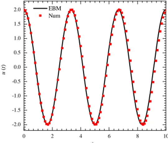
Its period can be written in the form:
0 2 4 6 8 10 -2.0
-1.5 -1.0 -0.5 0.0 0.5 1.0 1.5 2.0
u
(
t)
time
EBM Num
Figure 6.1 Comparison between approximate solutions and numerical solutions form=1, A=2, ε=0.5, k1=
5, k2=5
0 2 4 6 8 10 12
-5 -4 -3 -2 -1 0 1 2 3 4 5
u
(
t)
time
EBM Num
Figure 6.2 Comparison between approximate solutions and numerical solutions form=3, A=5, ε=1, k1=
8, k2=16
TEBM = 2
π(4+3A2εη)
ω0 √
(4+3A2εη) (4+3A2ε) (6.18)
To further illustrate and verify the accuracy of this approximate analytical approach,
com-424
parison of the time history oscillatory displacement responses for the system with linear and
425
nonlinear springs in series with numerical solutions are depicted in Figures 6.1 and 6.2. Figures
426
6.1 and 6.2 represent the displacements of u(t)for a mass with different initial conditions and
427
spring stiffnesses.
428
429
Example 2 430
From Hamden [79], it is known that the free vibrations of an autonomous conservative
431
oscillator with inertia and static type fifth-order non-linearties is expressed by
¨
x+λx+ε1x2x¨+ε1xx˙2+ε2x4x¨+2ε2x3x˙2+ε3x3+ε4x5=0, (6.19)
With the initial conditions:
433
x(0)=A x˙(0)=0 (6.20)
Motion is assumed to start from the position of maximum displacement with zero initial
434
velocity. λ is an integer which may take values of λ = 1,0 or −1, and ε1, ε2, ε3andε4 are
435
positive parameters.
436
The solution of nonlinear equation with the Energy Balance method is:
437
¨
x+λx+ε1x2x¨+ε1xx˙2+ε2x4x¨+2ε2x3x˙2+ε3x3+ε4x5=0, (6.21)
in whichxandtare generalized dimensionless displacement and time variables, respectively.
438
Its Variational principle can be easily obtained:
439
x(0)=A, x˙(0)=0 (6.22)
in whichxandtare generalized dimensionless displacement and time variables, respectively.
440
Its Variational principle can be easily obtained:
441
J(x)=∫ t
0 (
−1
2x˙ 2(
1+ε1x2+ε2x4)+
λ
2x
2+ε3
4x
4+ε4
6 x
6)dt
(6.23)
Its Hamiltonian, therefore, can be written in the form:
442
H =1 2x˙
2(
1+ε1x2+ε2x4)+
λ
2x
2+ε3
4x
4+ε4
6 x
6 =λ
2A
2+ε3
4A
4+ε4
6 A
6
(6.24)
Or
443
R(t)= 1 2x˙
2(
1+ε1x2+ε2x4)+
λ
2x
2+ε3
4x
4+ε4
6 x
6−λ
2A
2−ε3
4A
4−ε4
6A
6
=0 (6.25)
Oscillatory systems contain two important physical parameters, i.e. the frequency ωand
444
the amplitude x(t)=Acosω t of oscillation,A. So let us consider such initial conditions:
445
x(0)=A, x˙(0)=0 (6.26)
Assume that its initial approximate guess can be expressed as:
446
x(t)=Acosωt (6.27)
Substituting Eq. (6.27) into Eq. (6.25) yields:
R(t)= 1
2(−Asinωt) 2(
1+ε1(Acosωt)2+ε2(Acosωt)4)+
λ
2(Acosωt) 2
+ε3
4 (Acosωt)
4
+ε4
6(Acosωt) 6−λ
2A
2−ε3
4A
4−ε4
6 A
6=0
(6.28)
Which trigger the following results
448
ω= √
2
Asinωt
¿ Á Á Á Àλ2(A
2−(Acosωt)2)+ε3 4 (A
4−(Acosωt)4)+ε4 6 (A
6−(Acosωt)6)
1+ε1(Acosωt) 2
+ε2(Acosωt)
4 (6.29)
If we collocate at ωt= π
4 , we obtain:
449
ωEBM = √
3 3
√
12λ+9ε3A2+7ε4A4 4+2ε1A2+ε2A4
(6.30)
Substituting Eq. (6.30) into Eq. (6.27) yields:
450
x(t)=Acos⎛ ⎝
√ 3 3
√
12λ+9ε3A2+7ε4A4 4+2ε1A2+ε2A4
t⎞
⎠ (6.31)
The numerical solution with Runge-Kutta method for nonlinear equation is:
451
˙
x1=x2 x1(0)=A (6.32)
And
452
˙
x2=−
1 1+ε1x21+ε2x41
(λx1+ε1x1x22+2ε2x31x 2
2+ε3x31+ε4x51), x2(0)=0 (6.33)
Motion is assumed to start from the position of maximum displacement with zero initial
453
velocity. λIs an integer which may take values ofλ=1,0or−1, andε1, ε2, ε3andε4 are positive
454
parameters .The values of parametersε1, ε2, ε3andε4associated for a mode is shown in Table
455
6.1.
456
Table 6.1 Values of dimensionless parametersεiin Eq.(6.31)for a mode
Mode ε1 ε2 ε3 ε4
1 0.326845 0. 129579 0. 232598 0. 087584 2 1.642033 0.913055 0.313561 0.204297 3 4.051486 1.665232 0.281418 0.149677
It can be seen from Figures 6.3-6.4 EBM results have a good agreement with the numerical
457
solution for 3 modes.Figures show the motion of the system is a periodic motion and the
458
amplitude of vibration is a function of the initial conditions.
0 2 4 6 8 10 12 -1.0
-0.5 0.0 0.5 1.0
x
(t
)
time EBM
RKM
Figure 6.3 The Comparison between energy balance method solution and the numerical solution (Runge-Kutta method), withλ=1,A=1 for mode-1.
460
Example 3 461
Consider a straight Euler-Bernoulli beam of lengthL, a cross-sectional area A, the mass
462
per unit length of the beam m, a moment of inertia I, and a modulus of elasticity E that
463
is subjected to an axial force of magnitude P as shown in Fig.6.6. The equation of motion
464
including the effects of mid-plane stretching is given by:
465
m∂
2w′
∂t′2 +EI
∂4w′ ∂x′2 +P¯
∂2w′ ∂x′2 −
EA
2L
∂2w′ ∂x′2 ∫
L
0 (
∂2w′ ∂x′2)
2
dx′
=0 (6.34)
For convenience, the following non-dimensional variables are used:
466
x=x′/L,w=w′/ρ ,t=t′(EI/ml4)1/2, P =P L¯ 2/EI (6.35)
Where ρ =(I/A)1/2 is the radius of gyration of the cross-section. As a result Eq. (6.34)
467
can be written as follows:
468
∂2w
∂t2 +
∂4w
∂x4 +P
∂2w
∂x2 − 1 2
∂2w
∂x2 ∫ L
0 (
∂2w
∂x2) 2
dx=0 (6.36)
Assuming w(x, t)=V(t)φ(x)whereφ(x)is the first eigenmode of the beam [189] and
ap-469
plying the Galerkin method, the equation of motion is obtained as follows:
470
d2V(t)
dt2 +(α1+P α2)V(t)+α3V
3(t)=0 (6.37)
The Eq. (6.37) is the differential equation of motion governing the non-linear vibration of
471
Euler-Bernoulli beams. The center of the beam is subjected to the following initial conditions:
0 2 4 6 8 10 12 14 -1.0
-0.5 0.0 0.5 1.0
x
(t
)
time EBM
RKM
Figure 6.4 The comparison between energy balance method solution and the numerical solution (Runge-Kutta method), withλ=1, A=1 for mode-2.
V(0) = ∆, dV(0)
dt =0 (6.38)
Where ∆ denotes the non-dimensional maximum amplitude of oscillation and α1, α2 and
473
α3are as follows:
474
α1=(∫ 1
0 (
∂4φ(x)
∂x4 )φ(x)dx) /∫ 1
0
φ2(x)dx (6.39a)
α2=(∫ 1
0 (
∂2φ(x)
∂x2 )φ(x)dx) /∫ 1
0 φ
2(x)dx (6.39b)
α3=⎛ ⎝(−
1
2)∫
1
0 ⎛ ⎝
∂2φ(x)
∂x2 ∫ 1
0 (
∂2φ(x)
∂x2 ) 2
dx⎞
⎠ φ(x)dx⎞⎠/∫ 1
0
φ2(x)dx (6.39c)
Variational formulation of Eq. (6.37) can be readily obtained as follows:
475
J(V)= ∫ t
0 (
−1
2
dV(t) dt +
1
2(α1+P α2)V 2(
t)+α3V4(t))dt . (6.40)
Its Hamiltonian, therefore, can be written in the form:
476
H=−1
2
dV(t) dt +
1
2(α1+P α2)V 2(
t)+α3V4(t) (6.41)
And
477
Ht=0= 1
2∆
2(α
1+P α2)+ 1
4α4∆
0 4 8 12 16 20 -1.0
-0.5 0.0 0.5 1.0
x
(t
)
time EBM
RKM
Figure 6.5 The comparison between energy balance method solution and numerical solution (Runge-Kutta method), withλ=1, A=1 for mode-3.
Figure 6.6 A schematic of an Euler-Bernoulli beam subjected to an axial load.
Ht−Ht=0= 1 2
dV(t) dt +
1
2(α1+P α2)V 2(
t)+α3V4(t)− 1
2∆
2(
α1+P α2)− 1
4α4∆
4
(6.43)
We will use the trial function to determine the angular frequency ω, i.e.
478
V (t)=Acosω t (6.44)
If we substitute Eq. (6.46) into Eq. (6.45), it results the following residual equation
479
1
2(−∆ω sin(ωt)) 2
+1
2(α1+P α2) (∆ cos(ω t)) 2
+1
2α3(∆ cos(ωt)) 4
−1 2∆
2(α
1+P α2)−14α3∆4 =0
(6.45)
If we collocate atω t= π
4we obtain:
480
1
4∆
2ω2−1
4∆
2(α
1+P α2)− 3
16α3∆
4 =0 (6.46)
The non-linear natural frequency and the deflection of the beam center become as follows:
ωN L = √
4(α1+P α2)+3α3∆2
2 (6.47)
According to Eq. (6.49) and Eq. (6.46), we can obtain the following approximate solution:
482
V (t)=∆ cos( √
4(α1+P α2)+3α3∆2
2 t) (6.48)
Non-linear to linear frequency ratio is:
483
ωN L
ωL = 1
2 √
4(α1+pα2)+3α3∆2
√α
1+pα2
(6.49)
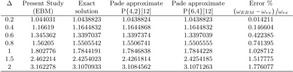
Table 6.2 shows the comparison of non-linear to linear frequency ratio (ωN L/ωL) ∆ Present Study Exact Pade approximate Pade approximate Error %
(EBM) solution P{4,2}[12] P{6,4}[12] (ωEBM−ωex) /ωex
0.2 1.044031 1.0438823 1.0438824 1.0438823 0.014211
0.4 1.16619 1.1644832 1.1644868 1.1644832 0.146604
0.6 1.345362 1.3397037 1.3397374 1.3397039 0.422385
0.8 1.56205 1.5505542 1.5506741 1.5505555 0.741395
1 1.802776 1.7844191 1.7846838 1.7844228 1.028712
1.5 2.462214 2.4254023 2.4261814 2.4254185 1.517775
2 3.162278 3.1070933 3.1084562 3.1071263 1.776077
0 2 4 6 8 10 12 14 16 18
-0.6 -0.4 -0.2 0.0 0.2 0.4 0.6
W
(t
)
time EBM
Exact
Figure 6.7 Comparison of analytical solution ofW(t)based on timewith the exact solution for simply supported beam,∆=0.6, α1=1, α2=0, α3=3
To show the accuracy of Energy Balance Method (EBM) , comparisons of the time history
484
oscillatory displacement response for Euler-Bernoulli beams with exact solutions are presented
485
in Figs. 6.7 and 6.8 .
0 1 2 3 4 5 6 7 8 -2.0
-1.5 -1.0 -0.5 0.0 0.5 1.0 1.5 2.0
W
(t
)
time
EBM Exact
Figure 6.8 Comparison of analytical solution ofW(t)based on timewith the exact solution for simply supported beam,∆=1.5, α1=1, α2=0, α3=3
It can be observed that the results of EBM require smaller computational effort and only a
487
first-order approximation leads to accurate solutions. The Influence ofα3on nonlinear to linear
488
frequency and α1are presented in figures 6.9 and 6.10. It has illustrated that Energy Balance
489
Method is a very simple method and quickly convergent and valid for a wide range of vibration
490
amplitudes and initial conditions. The accuracy of the results shows that the Energy Balance
491
Method can be potentiality used for the analysis of strongly nonlinear oscillation problems
492
accurately.
-3 -2 -1 0 1 2 3 1.0
1.2 1.4 1.6 1.8 2.0
ωNL
/
ωL
∆ α3=0.2
α3=0.4
α3=0.6
α3=0.8
α3=1.0
Figure 6.9 Influence ofα3 on nonlinear to linear frequency base on∆forα1=1, α2=0.5, p=2
-3 -2 -1 0 1 2 3
1.0 1.2 1.4 1.6 1.8 2.0 2.2 2.4 2.6
ωNL
/
ωL
∆ α1=0.5 α1=1.0 α1=1.5 α1=2.0 α1=2.5
Figure 6.10 Influence ofα3 on nonlinear to linear frequency base on∆forα2=1, α3=3, p=3
7 PARAMETER –EXPANSION METHOD (PEM) 494
Various perturbation methods have been applied frequently to analyze nonlinear vibration
495
equations. These methods are characterized by expansions of the dependent variables in power
496
series in a small parameter, resulting in a collection of linear deferential equations which can
497
be solved successively. He proposed the parameter expanding method for the first time in his
498
review article [100].The main property of the method is to use parameter-expansion technique
499
to eliminate the secular terms and to achieve the frequency. PEM was successfully applied to
500
various engineering problems [8, 42, 69, 97, 103, 118, 134, 147, 161, 190, 195–197, 201].
7.1 Basic idea of Parameter–Expansion Method 502
In order to use the PEM, we rewrite the general form of Duffing equation in the following
503
form[100]:
504
¨
u+ε u+1. N(u, t)=0. (7.1)
Where N(u, t) includes the nonlinear term. Expanding the solutionu,εas a coefficient of
505
u,and 1 as a coefficient of N(u, t), the series ofp can be introduced as follows:
506
u=u0+p u1+p1u2+p2u3+... (7.2)
ε=ω2+p d1+p1d2+p2d3+... (7.3)
1=p a1+p1a2+p2a3+... (7.4)
Substituting (7.2)-(7.4) into (7.1)and equating the terms with the identical powers ofp, we
507
have
508
p0∶u¨0+ω2u0=0 , (7.5)
p1∶u¨
1+ω2u1+d1u0+a1N(u0, t)=0 ,
⋮ (7.6)
Considering the initial conditions u0(0) = A and ˙u0(0) = 0, the solution of (7.5) is u0 =
509
Acos(ω t). Substitutingu0into (7.6), we obtain
510
p1∶u¨1+ω2u1+d1Acos(ω t)+a1N(A cos(ω t), t)=0 . (7.7)
For achieving the secular term, we use Fourier expansion series as follows:
511
N(Acos(ω t), t)=
∞
∑
n=0
b2k+1cos((2k+1)ωt). (7.8)
Substituting (7.8) into(7.7) yields;
512
p1∶u¨1+ω2u1+(d1A+ a1b1)cos(ω t)=0 . (7.9)
For avoiding secular term, we have
513
(d1A+a1b1)=0 . (7.10)
Setting p=1 in (7.3)and (7.4) ,we have:
514

![Figure 4.2 Nonlinear free vibration of a system of mass with serial linear and Nonlinear stiffness on a frictionless contact surface[185]](https://thumb-eu.123doks.com/thumbv2/123dok_br/18884604.423527/20.892.96.814.76.1040/figure-nonlinear-vibration-nonlinear-stiffness-frictionless-contact-surface.webp)