ANALYTICAL AND NUMERICAL
ANALYSIS OF MHD
BOUNDARY-LAYER FLOW OF AN
INCOMPRESSIBLE
UPPER-CONVECTED MAXWELLFLUID
M. RAHIMI EOSBOEE*
Department of Mechanical Engineering, Faculty of Engineering, Urmia University, Urmia, 57169-33111, Iran
N. POURMAHMOUD, I. MIRZAIE, P. MOHAJERI KHAMENEH, S. MAJIDYFAR Department of Mechanical Engineering, Faculty of Engineering, Urmia University,
Urmia, 57169-33111, Iran
D. D. GANJI
Department of Mechanical Engineering, Babol University of Technology, Babol, P. O. Box 484, Iran.
Abstract:
In this study magnetohydrodynamics (MHD) boundary layer flow of an upper-convected Maxwell fluid has been investigated. Similarity transformation has been used to reduce the governing differential equations into an ordinary non-linear differential equation. homotopy perturbation Method (HPM) has applied to solve this developed nonlinear equation. In this article firstly, the basic idea of the HPM for solving nonlinear differential equations is briefly introduced and then it is employed to derive solution of nonlinear governing equation of MHD boundary layer flow with highly nonlinear term. The obtained results from HPM have been compared with numerical Boundary Value problem Method (BVP) to verify the accuracy of the proposed method. The effects of the Hartman number (M) and Deborah number (β) for various conditions have been shown through graphs.
Keywords: MHD maxwell fluid boundary layer flow; Homotopy perturbation method (HPM); Numerical boundary value problem method (BVP).
1. Introduction
Magnetohydrodynamics (MHD) is a part of the mechanics of continuous media which studies the motion of electrically conducting media in the presence of a magnetic field. MHD is essential in plasma physics and astrophysics and the earliest investigations in this area was conducted by Alfven [1] around 1940 (Nobelprize in physics 1970). Most of the main applications of MHD in nature are the Earth’s core and solar flares, and also it has many applications in engineering such as the electromagnetic casting of metals and the confinement of plasmas [2].
In the recent decades, non-Newtonian fluid flows have attracted considerable attention due to their important engineering applications. Unlike the Newtonian fluids, the flows of non-Newtonian fluids don’t obey the Navier-Stokes theory. There are several constitutive equations that have been proposed to various types of non-Newtonian fluids. One type of fluids in which the relaxation type phenomena taken into account is known as Maxwell model. This kind of fluid has significant application in viscoelastic problems which have small dimensionless relaxation time [3-5]. The present work has been undertaken to provide an analytical and numerical solution for MHD boundary layer flow of an upper-convected Maxwell fluid.
upper-convected Maxwell fluid has been studied. In 1999, the initial works in HPM was studied by J. H. He [6-10] and after that these investigations inspired a lot of researchers [11-20] to solve nonlinear equations with this method. It was shown by many authors that this method could provide improvements in numerical techniques.
This paper is organized as follows: Section 2 is devoted to the description of the problem. In section 3, the mathematical model of this method is introduced and then its application in this model is studied. Section 4 deals with the results of the HPM solution. Section 5 gives the conclusions.
2. Description of the problem
In this section the flow equations and constitutive relations are given. Two-dimensional MHD flow of an incompressible upper-convected Maxwell fluid has been investigated in this paper. The two independent velocity components are u (in x-direction) and v (in y-direction) and B0 is a uniform static magnetic field in y-direction. For either laminar or turbulent flow, the two-dimensional continuity equation is given by:
0
y v x u
(1) The constitutive equation for the Cauchy stress (T) in a Maxwell fluid [21] is expressed, as:
T pI S (2)
Where the extra stress tensor (S) is calculated [21] by eq. (3), as: 1
dS
S LS SL A
dt
(3)
In which "µ" is the viscosity, "λ" is the relaxation time and the first Rivlin–Ericksen tensor (A1) is defined by [21]:
1
A V V (4)
Momentum differential equation is given by: V p f dt dV
b
2
(5)
There is a magnetic body force on the x-direction and is called Lorenz force [22,23] that its relation is shown below, as:
Lorenz force
J
B
(6)Where "J" is the electric current density and "B" is the magnetic flux. The current density is obtained by Ohm’s law [22,23], as:
E V B
J (7)
Where "σ" is the electrical conductivity and "E" is the electric field. A magnetic field in the medium will be induced by motion of an electrically conducting fluid in an applied magnetic field. The summation of the applied and induced magnetic field will produce the total field. The magnetic Reynolds number (Rem=σ µm U L
with characteristic values of velocity and length, U and L, and µm is magnetic permeability) was used to
describe the relative strength of the induced field. In order to neglect the induced magnetic field, it should be assumed that the magnetic Reynolds number has a small value [24]. According to above assumptions, the electric field is zero because the external electric field and the effect of polarization of the ionized fluid are assumed to be zero. Hence:
0
E (8)
By substituting Eq. (8) into Eq. (7) and then by inserting the obtained result in Eq. (6), yields:
V B
B B Vfbx
2 0
, (9)
2
0 S S
1 B 1 xx xy
u u p
u v u
x y x x y
(10)
S S 1 1 yx yy
v v p
u v
x y y x y
(11)
Where "ρ" is the fluid density, "σ" is the electrical conductivity and "Sxx", "Sxy", " Syx" and "Syy" are the
components of the extra stress tensor. By using the boundary layer approximations [25] and in the absence of a pressure gradient, the equation for the MHD boundary layer flow of an incompressible upper-convected Maxwell fluid is transformed to Eq. (12), as:
2
2 2 2 2
2 2 0
2 2 2 2
B
u u u u u u
u v u v uv u
x y x y x y y
(12)
Also the boundary condition for this problem is as follows:
, 0 0
0
u U v at y
u as y
(13)
By introducing the stream function ψ: , u v y x
(14)
The continuity equation is automatically satisfied and Eq. (12) reduces to:
2 2
2
2 2 3 3 3 3
0
2 3 2 3 2 2
B
y x y x y y y y x y x y y x x y
(15)
Base on Eq. (16), Similarity transformation is used to reduce the governing differential equation reduces to an ordinary non-linear differential equation.
,
U
y xU f
x
(16)
The Eqs. (15) and (13) become:
''' 2 ' '' ' '' 2 ''' '2 ''
2
f
2
M f
f f
2
f f f
f
f
f
f
0
(17)
' '
0, 1 0
0
f f at
f as
(18)
Here M2=σB02x/ρU and β=λU/2x. The homotopy perturbation method is exerted to solve Eqs. (17) and (18) in
the next section.
3. Homotopy Perturbation Method (HPM)
3.1.Basic idea of HPM
( ) ( ) 0,
A u f r rΩ, (19)
Subject to boundary condition:
( , ) 0 ,
B u u n rΓ, (20)
Where "A" is a general differential operator, "B" is a boundary operator, f(r) is a known analytical function, "Γ" is the boundary of domain "Ω" and ∂u/∂n denotes differentiation along the normal drawn outwards from"Ω". The operator "A" can, generally speaking, be divided into two parts: a linear part "L" and a nonlinear part "N". Therefore Eq. (19) can be rewritten as follows:
,
0
)
(
)
(
)
(
u
N
u
f
r
L
(21)In case that the nonlinear Eq. (19) has no “small parameter”, we can construct the following homotopy:
,
0
))
(
)
(
(
)
(
)
(
)
(
)
,
(
v
p
L
v
L
u
0
pL
u
0
p
N
v
f
r
H
(22)Where,
r,p :
0,1 R, (23)
In Eq. (22), pא[0,1] is an embedding parameter and u0 is the first approximation that satisfies the boundary
condition. We can assume that the solution of Eq. (22) can be written as a power series in "p", as following: ,
... 2 2 1
0
p p (24)And the best approximation for solution is:
,
...
lim
1
0
1
2
p
u
(25)When, Eq. (22) correspond to Eq. (19) and Eq. (25) becomes the approximate solution of Eq. (19) some interesting results have been attained using this method. Convergence and stability of this method was shown in Ref [26].
3.2. Solution with Homotopy Perturbation Method
In order to solve Eq. (17), the HPM is exerted to this equation. According to the HPM, the homotopy form of Eq. (17) is constructed as follows:
''' 2 '
''' 2 ' '' ' '' 2 ''' ' 2 ''
, 1 2 2
2 2 2 0
H f p p f M f
p f M f f f f f f f f f f
(26)
2
0 1 2
( ) ( ) ( ) ( ) ...
f f p f p f (27)
By substituting Eq. (27) into Eq. (26) and collect H (f , p) and then by inserting the coefficients of "p" equal to zero, we have:
3
0 2
0 3 0
0 0 0
: 2 2 0
0 0, 0 1, 0
d d
p M f f
d d
d d
f f f
d d (28)
2 2 1 20 2 0 1 0 0 2 0
2
3 3 2
2
0 3 0 3 1 0 2 0
0
: 2 2
- 2 0
0
d d d d
p f f M f f f f
d d d d
d d d d
f f f f f
d d d d
f
0 00, d f 0 0, d f 0
d d
4 4
4 4
0 4 4
M M
M M
M M
e e e e
f
M e e
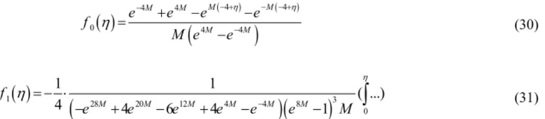
(30)
1 3
28 20 12 4 4 8
0
1 1
( ...)
4 M 4 M 6 M 4 M M M 1
f
e e e e e e M
(31)f1 (η) is too long that is not shown in this paper. By substituting Eqs. (30) and (31) into Eq. (27), yields:
4 4
4 4
4 4
3
28 20 12 4 4 8
0
1 1
( ...)
4 4 6 4 1
M M
M M
M M
M M M M M M
e e e e
f
M e e
e e e e e e M
(32)4. Result and Discussion
In Fig. (1) the results of Homotopy Perturbation Method is compared with boundary value problem (BVP). Good accuracy of this method can be seen in figure (1) and table (1). It is very interesting that HPM with two stages converge to the results with a good accuracy.
Fig. 1. comparison between HPM and BVP for M=1, β=0.4
Table. 1. The results of HPM solution and Comparison of these results with BVP
η fHPM fBVP Error=│fHPM- fBVP│
0 0 0 0
0.5 0.38662 0.386325 0.000295
1 0.60613 0.605299 0.000831 1.5 0.72485 0.724257 0.000593
2 0.78562 0.786745 0.001125 2.5 0.81461 0.818662 0.004052
3 0.82698 0.834332 0.007352
3.5 0.83119 0.841253 0.010063
In Figs. (2-7), effects of Hartman number (M) and Deborah number (β) on the velocity components f and f ' have been investigated.
Effect of the Hartman number on the velocity components f and f ' has been shown In Figs. (2) and (3). It should be indicated that, these figures have been drawn for β=0.5. As it can be seen with an increase in the Hartman number, the velocity components f and f ' decrease gradually. It is concluded that with increasing in "M", magnetic body force will be increased and it lead to decrease in thickness of boundary layer.
Fig. 2. Effects of the Hartman number on the velocity component (f ) when β= 0.5
Fig. 3. Effects of the Hartman number on the velocity component (f '
) when β= 0.5
In Figs. (4–7) effect of the Deborah number (β) on the velocity components f and f'
Fig. 4. Effects of the Deborah number on the velocity component (f ) when M= 0
Fig. 5. Effects of the Deborah number on the velocity component (f '
) when M= 0
As it can be seen in Figs. (6) and (7) at high Hartman number (M > 0.5) with enlarging"β", f at low Deborah number increases and at high Deborah number firstly increases and then decreases. Also f ' at low Deborah number decreases and at high Deborah number firstly decreases and then increases. Figs. (6) and (7), have been drown for M=2.
Fig. 7. Effects of the Deborah number on the velocity component (f '
) when M= 2
5. Conclusion
In this study, MHD boundary layer flow of an upper-convected Maxwell fluid was investigated. The nonlinear equation was solved by Homotopy Perturbation Method and the influence of Hartman number and Deborah number was studied on the velocity field. The result of HPM was compared with BVP and it was observed that HPM with two stages was converged to the BVP results with a good accuracy. As it was obtained with an increase in the parameter "M"the boundary layer thickness was decreased gradually. Finally the effect of the parameter "β" was investigated on the velocity components f and f ' and it was deduced that the behavior of the velocity components at low Hartman number (0 ≤ M ≤ 0.5) is different with high Hartman number (M > 0.5). References
[1] Khater, A. H.; Callebaut, D. K.; Abdelhameed, T. N. (2006): Potential symmetry and invariant solutions of Fokker-Planck equation in cylindrical coordinates related to magnetic field diffusion in magnetohydrodynamics including the Hall current, Eur. Phys. J. B 50, pp. 17–21.
[2] Gurion, B. and et al. (1984): Single- and multi-phase flows in an electromagnetic field: energy, metallurgical, and solar applications, 4th Edition, American Institute of Aeronautics and Astronautics, preface.
[3] Fetecau, C.; Fetecau, C. (2003): The Rayleigh–Stokes problem for a fluid of Maxwellian type, Int. J. Non-Linear Mech. 38, pp. 603– 607.
[4] Fetecau, C.; Fetecau, C. (2005): Starting solutions for some unsteady unidirectional flows of a second grade fluid, Int. J. Eng. Sci. 43, pp. 781-789.
[5] Sadeghy, K.; Najafi, A.H.; Saffaripour, M. (2005): Sakiadis flow of an upper-convected Maxwell fluid, Int. J. Non-Linear Mech. 40, pp. 1220–1228.
[6] He, J.H. (2009): An elementary introduction to the homotopy perturbation method, Computers & Mathematics with Applications, Volume 57, Issue 3, pp. 410-412.
[7] He, J.H. (1998): Approximate analytical solution for seepage flow with fractional derivatives in porous media, J. Comput. Math. Appl. Mech. Eng , pp. 167:57-68.
[8] He, J.H. (2000): A review on some new recently developed nonlinear analytical techniques, Int J Non-linear Sci Numer Simul, 1, pp. 51-70.
[9] He, J.H. (2001): Modified Lindstedt–Poincare methods for some non-linear oscillations. Part III: double series expansion, Int. J. Non- linear Sci Numer Simul, 2:317-20.
[10] He, J.H. (2005): Homotopy perturbation method for bifurcation on nonlinear problems, Int. J. Non-linear Sci. Numer. Simul, 6:207-8. [11] Ganji, D. D.; Rajabi, A. (2006): Assessment of homotopy-perturbation and perturbation methods in heat radiation equations, Internat.
Comm. Heat Mass Transfer, 33, pp. 391-400.
[12] Ganji, D. D.; Sadighi, A. (2006): Application of He’s Homotopy–perturbation Method to Nonlinear Coupled Systems of Reaction– diffusion Equations, Int. J. Nonl. Sci. and Num. Simu, 7(4), pp. 411-418.
[13] Ariel, P.D.; Hayat, T.; Asghar, S. (2006): Homotopy perturbation method and axisymmetric Flow over a stretching sheet, Internat J. Nonlinear Sci. Numer. Simul, 7(4), pp. 399-406.
[14] Hosein Nia, S.H.; Ranjbar, A.N.; Ganji, D. D.; Soltani, H.; Ghasemi, J. (2008): Maintaining the stability of nonlinear differential equations by the enhancement of HPM, Physics Letters A, 372(16), pp. 2855-2861.
[15] Ganji, Z.Z.; Ganji, D. D. (2008): Approximate Solutions of Thermal Boundary-layer Problems in a Semi-infinite Flat Plate by using He's Homotopy Perturbation Method, International Journal of Nonlinear Sciences and Numerical Simulation, 9(4), pp. 415-422. [16] Beléndez, A.; Beléndez, T.; Márquez, A.; Neipp, C. (2008): Application of He's homotopy perturbation method to conservative truly
nonlinear oscillators, Chaos, Solitons & Fractals, 37(3), pp. 770-780.
[18] Siddiqui, A.M.; Zeb, A.; Ghori, Q. K.; Benharbit, A. M. (2008): Homotopy perturbation method for heat transfer flow of a third grade fluid between parallel plates, Chaos, Solitons & Fractals, 36(1), pp. 182-192.
[19] Zhang, B.G.; Li, S.Y.; Liu, Z.R. (2008): Homotopy perturbation method for modified Camassa-Holm and Degasperis-Procesi, Physics Letters A, 372(11), pp. 1867-1872.
[20] Zhang, L.N.; He, J. H. (2006): Homotopy perturbation method for the solution of the electrostatic potential differential equation, Mathematical Problems in Engineering, Art. No. 83878.
[21] Hayat, T.; Sajid, M. (2007): Homotopy analysis of MHD boundary layer flow of an upper-convected Maxwell fluid, International Journal of Engineering Science, 45, pp. 393–401.
[22] Paris, D. T.; Hurd, F. K. (1969): Basic electromagnetic theory, McGraw-Hill, New York.
[23] Plonsey, R.; Collin, R. E. (1982): Principles and applications of electromagnetic fields, 2th edition, McGraw-Hill, New York. [24] Wang, Y.; Hayat, T.; Hutter, K. (2005): On non-linear magnetohydrodynamic problems of an Oldroyd 6-constant fluid, International
Journal of Non-Linear Mechanics, 40, pp. 49– 58.
[25] Schichting, H. (1964): Boundary Layer Theory, sixth ed., McGraw-Hill, New York.