Abstract—This paper summarizes the related works about feature selection via the induction of Markov blanket which can be traced back to 1996, and the concept of Markov blanket itself firstly appeared even earlier in 1988. Our review not only covers a series of published algorithms, including KS, GS, IAMB and its variants, MMPC/MB, HITON-PC/MB, Fast IAMB, PCMB and IPC-MB (ordered as their appearing time), but why they were invented and their relative advantage as well as disadvantages, from both theoretical and practical viewpoint. Besides, it is noticed that all of these mentioned works are all constraint learning which depends on conditional independence test to induce the target, instead of via score-and-search, another mainstream manner as applied in the structure learning of one closely related concept, Bayesian network. Bing the first one, we discuss the cause which uncovers that this choice is not accidental, though not in a formal way. The discussion covered here is believed a valuable reference for academic researchers as well as applicants.
Index Terms—Feature selection, Markov Blanket.
I. INTRODUCTION
As of 1997, when a special issue (of the journal of Artificial Intelligence) on relevance including several papers on variable and feature selection was published [1], [2], few domains explored used more than 40 features. The situation has changed considerably in the past decade, and currently domains involving many more variables, hundreds to
Shunkai Fu is with the Computer Engineering Department, Ecole
Polytechnique de Montreal, Canada, and the Computer Science and
Technology College, Donghua University, China (e-mail: shunkai.fu@
polymtl.ca)
Michel C.Desmarais is with the Computer Engineering Department,
Ecole Polytechnique de Montreal, Canada (e-mail:
thousands, are becoming common. Therefore, feature selection has been an active research area in pattern recognition, statistics and data mining communities. The main idea of feature reduction is to select a subset of input variables by eliminating features with little or no predictive ability, but without scarifying the performance of the model built on the chosen features. It is also known as variable selection, feature reduction, attribute selection or variable
subset selection. By removing most of the irrelevant and
redundant features from the data, feature reduction brings many potential benefits to us:
Alleviating the effect of the curse of dimensionality to improve prediction performance;
Facilitating data visualization and data understanding, e.g. which are the important features and how they are related with each other;
Reducing the measurement and storage requirements;
Speeding up the training and inference process;
Enhancing model generalization.
A principle solution to the feature reduction problem is to determine a subset of features that can render of the rest of whole features independent of the variable of interest [3], [4], [5]. From a theoretical perspective, it is known that optimal feature reduction for supervised learning problems requires an exhaustive search of all possible subsets of features of the chosen cardinality, of which the complexity is known as exponential function of the size of whole features. In practice, the target is demoted to a satisfactory set of features instead of an optimal set due to the lack of efficient algorithms.
Feature selection algorithms typically fall into two categories, feature ranking and subset selection. Feature ranking ranks all variables by a metric and eliminates those that do not achieve an adequate score. Selecting the most relevant variables is usually suboptimal for building a
Markov Blanket based Feature Selection: A
Review of Past Decade
predictor, particularly if the variables are redundant. In other words, relevance does not imply optimality [2]. Besides, it has been demonstrated that a variable which is irrelevant by itself can provide a significant performance improvement when taken with others [2], [6].
Subset selection, however, evaluates a subset of features that together have good predictive power, as opposed to sorting variables according to their individual relevance. Essentially it can be divided into wrappers, filters and embedded [6]. In the wrapper approach, the feature selection
algorithm conducts a search through the space of possible combination of features and evaluates each subset by utilizing the learning algorithm of interest as a black box [2]. Wrappers can be computationally expensive because model training and cross-validation must be repeated over each feature subset, and the outcome is tailored to a particular model. Filters are similar to wrappers in the search approach, but instead of evaluating against a predictor, a simple filter is utilized as preprocessing. Therefore, filters work independent of the chosen predictor. However, filters have the similar weakness as feature ranking since they imply that irrelevant features are useless though it is proved not true [2], [6]. Embedded methods perform variable selection in the process of training and are usually specific to given learning algorithms. Compared with wrappers, embedded methods may be more efficient in several respects: they make better use of the available data without having to split the training data into a training and validation set; they reach a solution faster by avoiding retraining a predictor from scratch for every variable subset to investigate [6]. Embedded methods are found in decision trees such as CART, for example, which have a built-in mechanism to perform variable selection [7].
Koller and Sahami (KS) [3] first showed that the Markov blanket (MB) of a given target variable is the theoretically optimal set of features to predict ’s value, although Markov blanket itself is not a new concept and can be traced back to the work of Pearl [8] in 1988. Based on the findings that the full knowledge of is enough to determine the probability distribution of and that the values of all other variables become superfluous, inducing actually is a procedure of feature selection [3, 4, 9]. From our point of view, Markov blanket based feature selection can be categorized into filters, which means that it works independently of the later processing. Therefore, it is
expected to be much more efficient than wrapper approaches. Furthermore, it conquers the defect of conventional filters, with an output containing only relevant and useful attributes. Compared with embedded ways, it is obviously a more general choice and could work with all learning algorithms.
Since KS’s work in 1996, there are several attempts to make the learning procedure more efficient and effective, including GS (Grow-Shrink) [10], IAMB (Iterative Associative Markov Blanket) and its variants [4, 9], MMPC/MB (Max-Min Parents and Children/Markov Blanket) [11], HITON-PC/MB [12], Fast-IAMB [13], PCMB (Parent-Children Markov Blanket learning) [5] and IPC-MB (Iterative Parent and Children Markov Blanket learning, or with another name BFMB) [14, 15].
In Section 2, the Markov blanket itself is defined, as well as its relation with Bayesian Network. Then, in Section 3, we review all major algorithms on learning Markov blanket. In Section 4, we discuss why all these algorithms are constraint learning, instead of score-and-search, another primary family of algorithms for inducing Bayesian Network. We conclude with a summary about all algorithms covered in this paper for quick reference.
II. BAYESIAN NETWORK AND MARKOV BLANKET Bayesian network is a graphical tool that compactly represents a joint probability distribution over a set of random variables using a directed acyclic graph (DAG) annotated with conditional probability tables of the probability distribution of a node given any instantiation of its parents. Therefore, the graph represents qualitative information about the random variables (conditional independence properties), whiles the associated probability distribution, consistent with such properties, provides a quantitative description of how the variables related to each other. One example of Bayesian network is shown in Fig.1. The probability distribution and the graph of a Bayesian network are connected by the Markov condition property: a node is conditionally independent of its non-descendants, given its parents.
Given the faithfulness assumption, the Markov blanket of is unique, and it becomes trivial to retrieve it from the corresponding Bayesian network over the problem domain . It is known as composed of ’s parents, children and spouses (Fig.1). However, this requires the Bayesian network to be ready in advance. Indeed, traditionally, we have to learn the target Bayesian network first to get the Markov blanket of some variable, but the structure learning of Bayesian network is known as NP-complete problem. Therefore, an ideal solution will allow us to induce the Markov blanket but without having to have the whole Bayesian network ready first, which, potentially, reduces the time complexity greatly so that we can solve larger scale of problem with the same computing resource.
Fig.1. An example of a Bayesian network. The are the variables in
gray, while additionally includes the texture-filled variable O.
Definition 2 Markov Blanket (Probability viewpoint). Given the faithfulness assumption, the Markov blanket of T is a minimal set conditioned on which all other nodes are independent of T, i.e.∀X U\MB T \ T, I X, T|MB T .
Definition 3 Markov Blanket (Graphical viewpoint). Given the faithfulness assumption, the Markov blanket of T is identical to T’s parents, children and children’ parents (spouses), i.e. MB T Pa T ⋃Ch T ⋃Sp T .
Theorem 1. If a Bayesian network G is faithful to a joint probability distribution P, then: (1) There is an edge between the pair of nodes X and Y iff. X and Y are conditionally dependent given any other set of nodes; (2) for each triplet of nodes X, Y and Z in G such that X and Y are adjacent to Z but X is not adjacent to Y, X → Z ← Y is a subgraph of G iff. X and Y are dependent conditioned on every other set of nodes that contains Z [17].
Given the faithfulness assumption, Definition 2 and Definition 3 define the Markov blanket from probability and
graphical view respectively.
Definition 3 plus Theorem 1 are the topology information as referred by more recent and finer algorithms such as MMPC/MB, HITON-PC/MB, PCMB and IPC-MB. Of course, faithfulness assumption is the basis for all, including GS, IAMB and its variants. Lucky enough, the vast majority of distributions are faithful in the sample limit [18].
III. ALGORITHMS FOR LEARNING MARKOV BLANKET (1996 – PRESENT)
A. KS
Pearl is the first one to define the concept and study the property of Markov blanket in his early work on Bayesian network [8]. However, Koller and Sahami’s work towards optimal feature selection is the original one to recognize that Markov blanket of the target of interest is the theoretically optimal set of features to predict its value [3]. Their finding attracted many following trials aiming at inducing the Markov blanket with better performance in the past decade.
Koller and Sahami proposed a theoretically justified framework for optimal feature selection based on using cross-entropy to minimizing the amount of predictive information lost during feature elimination [3]. They also proposed one approximate algorithm based on their theoretical model, and this algorithm is referred as KS by many since then. KS is the first algorithm for feature selection to employ the concept of Markov blanket. Although it is theoretically sound, the proposed algorithm itself doesn’t guarantee correct outcome. KS algorithm requires two parameters: (1) the number of variables to retain, and (2) the maximum number of variables the algorithm is allowed to condition on. These two limits are helpful to reduce the search complexity greatly, but with a sacrifice of correctness [4], [5].
B. GS
them from becoming more widespread. These two disadvantages are: exponential execution time and proneness to errors in dependence tests used. The former one is addressed in two ways. One is by identifying the local neighborhood of each variable in the Bayesian network as a pre-processing step in order to facilitate the recovery of the local structure around each variable in polynomial time under the assumption of bounded neighborhood size. The second, randomized version goes one step further, employing a user-specific number of randomized tests in order to ascertain the same result with high probability. The second disadvantage of this research approach, namely proneness to errors, is also addressed by the randomized version, by using multiple data sets and Bayesian accumulation of evidence.
Like the constraint-based learning algorithm, GS depends on two basic assumptions, faithfulness and correct/reliable conditional independence (CI) test. Here, the second assumption is required in practice since only when the number of observations is enough, the result of one statistical testing would be trustable. Actually, these two assumptions are also the basis of the following algorithms. As its name indicates, GS proceeds in two steps, growing greedily first then shrinking by removing false positives. It is the first algorithm proved correct, but it is not efficient and can’t scale to large scale applications. However, the soundness of the algorithm makes it a proven subject for future research.
In [10], Margaritis and Thrun also proposed one randomized version of GS algorithm to solve problems involving large amount of variables or variables with many possible values. It requires manually defined parameter to reduce the number of conditional tests, similar to KS algorithm; hence, it cannot guarantee correct output, and it is ignored without further discussion.
C. IAMB and Its Variants
IAMB was proposed in 2003 for classification problems in microarray research where thousands of attributes are quite common. It is an algorithm based on the same two assumptions of GS, sound in theory and especially simple in implementation. IAMB algorithm is structurally similar to GS, consisting of two phases – growing and shrinking. However, there is one important difference: GS orders the variables when they are considered for inclusion in the first
step, according to their strength of association with given the empty set. It then admits into candidate the next variable in the ordering that is not conditionally independent with given the current . One problem with this heuristic is that when the contains spouses of , the spouses are typically associated with very weakly given the empty set and are considered for inclusion in the late in the first phase (associations between spouses and are only through confounding/common descendant variables, thus they are weaker than those ancestors’ associations with ). In turn, this implies that more false positives will enter during the first step and the conditional tests of independence will become unreliable much sooner than when using IAMB’s heuristic. In IAMB, it reorders the set of attributes each time a new attribute enters the blanket in the growing phase based on updated CI testing results, which allows IAMB to perform better than GS since fewer false positives will be added during the first phase [4, 13].
In spite of the improvement, IAMB is still not data efficient since its CI tests may conditioned on the whole or even larger set due to its design, though this is not necessary as discovered by later work. This point is also noticed by its authors, and several variants of IAMB were proposed, like interIAMB, IAMBnPC and their combined version interIAMBnPC [9]. InterIAMBnPC employs two methods to reduce the possible size of the conditioning sets: (1) it interleaves the growing phase of IAMB with the pruning phase attempting to keep the size of as small as possible during all steps of the algorithm’s execution; (2) it substitutes the shrinking phase as implemented in IAMB with the PC algorithm instead. InterIAMB and IAMBnPC are similar to InterIAMBnPC but they only either interleave the first two phases or rely on PC for the backward phase respectively.
D. MMPC/MB
The overall MMMB algorithm is composed of two steps. Firstly, it depends on MMPC to induce which are directly connected to , i.e. . Then it attempts to identify the remaining nodes, i.e. spouses of . The spouses of are the parents of the common children of , which suggests that they should belong to ∪ . So, MMPC is applied to each to induce ’s parents and children, which are viewed as spouse candidates which contains false ones to be filtered out with further checking. To determine if ∪ is a spouse, we actually need to recognize the so-called v-structure, i.e.
→ ← . Therefore, the underlying connectivity is critical for us to do the induction, and Theorem 1 tells us how to determine the corresponding connectivity.
Although the algorithm MMPC/MB is proved not sound by Pena et al. [5], the proposed direction gets recognized by many. HITON-PC/MB, PCMB and IPC-MB all follow the similar two-phase framework of MMPC/MB.
E. HITON-PC/MB
HITON-PC/MB [12] is also the work by the authors of IAMB, and can be viewed as a trial to further make the induction of Markov blanket more data efficient to meet the challenge in practice
As mentioned by the end of 3.4, HITON-PC/MB works in a similar manner as MMPC/MB, with the exception that it interleaves the addition and removal of nodes, aiming at removing false positives as early as possible so that the conditioning set is as small as possible. Unfortunately, HITON-PC/MB is also proved not sound in [5]. However, it is still viewed as another meaningful trial for an efficient learning algorithm of Markov blanket without having to learn the whole Bayesian network.
F. Fast-IAMB
Fast-IAMB [13] is the work by the author of GS too. Similar to GS and IAMB, Fast-IAMB contains a growing phase and a shrinking phase. During the growing phase of each iteration, it sorts the attributes that are candidates for admission to from most to least conditionally dependent, according to a heuristic function conditional statistical test). Each such sorting step is potentially expensive since it involves the calculation of the
test value between and each member of which contains those left un-checked. The key idea behind Fast-IAMB is to reduce the number of such tests by adding not
one, but a number of attributes at a time after each reordering of the remaining attributes following a modification of the Markov blanket. Fast-IAMB speculatively adds one or more attributes of highest test significance without resorting after each modification as IAMB does, which (hopefully) adds more than one true members of the blanket. Thus, the cost of re-sorting the remaining attributes after each Markov blanket modification can be amortized over the addition of multiple attributes.
The question arises: how many attributes should be added to the blanket in each iteration? The following heuristic is used in [13]: dependent attributes are added as long as the conditional independence tests are reliable, i.e. there is enough data for conducting them.
In conclusion, Fast-IAMB realizes a fast induction by adding greedily as many candidates as possible in the growing phase.
G. PCMB
Following the idea of MMPC/MB and HITON-PC/MB, PCMB [5] was also proposed to conquer the data inefficiency problem of IAMB, and, more importantly, it is the first such trial proved sound theoretically.
PCMB requires the same two assumptions as needed by MMPC/MB and HITON-PC/MB: faithfulness and correct statistical test. Similarly, PCMB induces MB via the recognition of direct connection, i.e. parents and children about any variable of interest, just like how MMPC/MB and HITON-PC/MB do, which may explain where its name comes from.
H. IPC-MB
IPC-MB [15], or BFMB in its first publication version [14], is the most recent progress as published on this topic, aiming at even better performance than PCMB. It has similar framework to MMPC/MB, HITON-PC/MB and PCMB by recognizing firstly those directly connected to , known as candidate parents and children; then, it repeats the local search given each candidate as found, which not only enables us to recognize those false positives, but candidate spouses. Correct spouses are recognized further based on the second point of Theorem 1.
Compared with PCMB, IPC-MB determines the connectivity of any pair of variables in a “smarter” manner, and the overall heuristic as followed by IPC-MB is described as below:
IPC-MB proceeds by checking and removing false positives. Considering that the size of is normally much smaller than , filtering out negatives is believed to be much easier a job than directly recognizing positives;
Recognizing and removing as many, and as early, negatives as possible is an effective way to reduce noise and to avoid conditioning on unnecessarily large conditioning set, which is the precondition for reliable CI tests and for the success of learning. Besides, it saves the computing time by prevent needless tests;
IPC-MB filters negatives by conditioning on empty set on. Then, one variable is allowed for the conditioning set, and the checking continues on. This procedure iterates with increased conditioning set, resulting with more and more negatives are removed. So, it is obvious that the decision on a negative is made with as small conditioning set as possible, and as early as possible as well, which is the most factor for the success of IPC-MB considering that the reliability of CI test is the most factor to influence the performance of such kind of algorithms.
IPC-MB is declared with best trade-off among all published works of this type, in terms of soundness, time efficiency, data efficiency and information found [15, 16].
IV. WHY ALL CONSTRAINT LEARNING
Regarding the structure learning of Bayesian network, there are two primary approaches, i.e. constraint-based
learning and score-and-search. With constraint-based learning, it depends on a series of conditional independence (CI) to induce a Bayesian network in agreement with test results. However, with score-and-search, it defines a global measure (or score) which evaluates a given Bayesian network model as a function of the data. Then, it searches the space of possible Bayesian network models with the goal of finding one with optimal score. In the past years, score-and-search approach has received more attention due to several known advantages [19].
With the fact that Markov blanket actually is part of the target Bayesian network given the faithfulness assumption, is it possible to apply these two mature frameworks in learning Markov blanket? Even though the score-and-search approach attracted more attention in the past decade over constraint learning to induce Bayesian network structure, it is constraint learning that more preferred and experimented by researchers on Markov blanket learning. IAMB and its variants, GS, MMPC/MB, HITON-PC/MB, PCMB and IPC-MB are all such examples. We believe this is not accidental even though there is no explicit explanation on the choice in published articles, so we are going to share with some to make up this loss, though not in a formal manner.
Given a problem on , we don’t know how many variables belonging to , saying nothing of which ones exactly. With search-and-score approach, we have to measure all possible subsets ∗⊑ , i.e. the power set of , of which the complexity is 2| |, NP-complete. KS algorithm executes in a similar manner, and it requires specifying the target size of . Though specifying the size of
could limit KS’s running in a predictable scale of space, obviously it may prevent KS from producing correct results since it is impossible to “guess” the exact size of the target each time. So, even assuming that we could define a perfect measure (or scoring mechanism), it is not acceptable in practice if we have to do the search in an exponentially expanding space. Therefore, a more affordable as well as sound solution to induce is expected. To achieve this goal, some additional guidance is needed to figure out a finer search strategy, i.e. “constraining” the search in a more efficient manner so that as much as possible fruitless effort can be avoided. With the property of Markov blanket, i.e. is independent of any conditioned on
\ , we may reduce the search space greatly and get a more efficient algorithm. IAMB is one such important progress, and it indeed excels the previous naïve approach, like KS, with obvious gain in efficiency. Since then, all effort began to follow the constraint learning approach, proposing one after another algorithm aiming at better performance with more and more heuristics introduced. Of course, the procedure is becoming more and more sophisticated, though it is not what we expect.
V. CONCLUSION
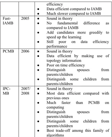
In this paper, we review the published algorithms on feature subset selection via the learning of Markov blanket given a target of interest. Those covered in the discussion are listed in Table 1 for quick reference.
To the best of our knowledge, IPC-MB achieves the best trade-off as compared with others, in term of effectiveness, time efficiency, data efficiency and topology information inferred.
Besides, we also discuss why all these algorithms are categorized as constraint-based learning, though not in a formal manner.
Table 1. Conclusion on the related algorithms for learning Markov Blanket
Name Pub. Year
Comments
KS 1996 Not sound
The first one of this type
Requires specifying MB size in advance
GS 1999 Sound in theory
Proposed to learn Bayesian network via the induction of neighbors of each variable
First proved such kind of algorithm Work in two phases: grow and shrink IAMB
and its variants
2003 Sound in theory Actually variant of GS Simple to implement Time efficient
Very poor on data efficiency
IAMB’s variants achieve better performance on data efficiency than IAMB
MMPC/ MB
2003 Not sound
The first to make use of the underling topology information
Much more data efficient compared to IAMB
Much slower compared to IAMB HITON
-PC/MB
2003 Not sound
Another trial to make use of the topology information to enhance data
efficiency
Data efficient compared to IAMB Much slower compared to IAMB
Fast-IAMB
2005 Sound in theory
No fundamental difference as compared to IAMB
Add candidates more greedily to speed up the learning
Still poor on data efficiency performance
PCMB 2006 Sound in theory
Data efficient by making use of topology information
Poor on time efficiency
Distinguish spouses from
parents/children
Distinguish some children from parents/children
IPC-MB
2007/ 2008
Sound in theory
Most data efficient compared with previous ones
Much faster than PCMB on computing
Distinguish spouses from
parents/children
Distinguish some children from parents/children
Best trade-off among this family of algorithms
REFERENCES
[1] Blum, A. and P. Langley, Selection of Relevant Features and
Examples in Machine Learning. Artificial Intelligence, 1997. 97(1-2).
[2] Kohavi, R. and G.H. John, Wrappers for Feature Subset Selection.
Artificial Intelligence, 1997. 97(1-2).
[3] Koller, D. and M. Sahami. Toward Optimal Feature Selection. in
ICML. 1996.
[4] Tsamardinos, I., C.F. Aliferis, and A.R. Statnikov. Time and sample
efficient discovery of Markov blankets and direct causal relations. in
the Ninth ACM SIGKDD International Conference on Knowledge
Discovery and Data Mining. 2003: ACM.
[5] Peña, J.M., et al., Towards scalable and data efficient learning of
Markov boundaries. International Journal of Approximate Reasoning
2007. 45(2).
[6] Guyon, I. and A. Elisseeff, An Introduction to Variable and Feature
Selection. Journal of Machine Learning Research, 2003. 3.
[7] Breiman, L., et al., Classification and Regression Trees. 1984:
Wadsworth.
[8] Pearl, J., Probabilistic reasoning in expert systems. 1988, San Matego:
Morgan Kaufmann.
[9] Tsamardinos, I., C.F. Aliferis, and A.R. Statnikov. Algorithms for
Large Scale Markov Blanket Discovery. in the Sixteenth International
Florida Artificial Intelligence Research Society Conference. 2003. St.
[10] Margaritis, D. and S. Thrun. Bayesian Network Induction via Local
Neighborhoods. in Advances in Neural Information Processing
Systems 1999. Denver, Colorado, USA: The MIT Press.
[11] Tsamardinos, I., L.E. Brown, and C.F. Aliferis, The max-min
hill-climbing Bayesian network structure learning algorithm Machine
Learning, 2006. 65(1): p. 31-78.
[12] Aliferis, C.F., I. Tsamardinos, and A.R. Statnikov. HITON: A novel
Markov blanket algorithm for optimal variable selection. in American
Medical Informatics Association Annual Symposium. 2003.
[13] Yaramakala, S. and D. Margaritis. Speculative Markov Blanket
Discovery for Optimal Feature Selection. in ICDM. 2005.
[14] Fu, S.-K. and M.C. Desmarais. Local Learning Algorithm for Markov
Blanket Discovery. in Australian Conference on Artificial
Intelligence. 2007. Gold Coast, Australia: Springer.
[15] Fu, S.-K. and M.C. Desmarais. Fast Markov Blanket Discovery
Algorithm Via Local Learning within Single Pass. in Canadian
Conference on AI. 2008. Windsor, Canada: Springer.
[16] Fu, S.-K. and M.C. Desmarais. Tradeoff Analysis of Different
Markov Blanket Local Learning Approaches. in Advances in
Knowledge Discovery and Data Mining, 12th Pacific-Asia
Conference (PAKDD). 2008. Osaka, Japan: Springer.
[17] Spirtes, P., C. Glymour, and R. Scheines, Causation, Prediction and
Search (2nd Edition). 2001: The MIT Press.
[18] Pearl, J., Causality: Models, Reasoning, and Inference. 2000:
Cambridge University Press.
[19] Heckerman, D. A Bayesian Approach to Learning Causal Networks.
in the Eleventh Annual Conference on Uncertainty in Artificial