S E M I - S U P E RV I S E D F E AT U R E S E L E C T I O N
frederico gualberto ferreira coelho
Thesis presented to the Electrical Engineering Post-Graduate Program of UFMG and to the “Commission Doctoral de Domaine des Sciences de l’Ingénieur” of UCL, in an Agreement for International joint supervision of PhD thesis, as partial fulfillment of the requirements for the degree of Philosophy Doctor of the “Universidade Federal de Minas Gerais” and the degree of Doctor in “Sciences de l’ingénieur” of “Université catholique de Louvain”
Jury:
Prof.A. Braga, Supervisor (UFMG - School of Engineering, Department of Electronics Engineering, LITC)
Prof.M. Verleysen, Supervisor (UCL - ICTEAM Institute, Machine Learning Group) Prof.F. Rossi, (Université Paris I Panthéon Sorbonne)
Prof.M. Vellasco, (PUC-RJ - Department of Electrical Engineering)
Prof.H. Yehia, (UFMG - School of Engineering, Department of Electronics Engineering) Prof.J. Lee, (UCL - ICTEAM Institute, Machine Learning Group)
Scholarship from CNPq during stay in Brazil - Proc. n°41818/2010-7 Scholarship from CAPES during stay in Belgium - Proc. n°1456/10-5
Universidade Federal de Minas Gerais - Université catholique de Louvain
Rapaduraé doce... mas não é mole não.
(Ditado popular de autoria desconhecida).
A B S T R A C T
As data acquisition has become relatively easy and inexpensive, data sets are becoming extremely large, both in relation to the number of variables, and on the number of instances. However, the same is not true for “labeled” instances . Usually, the cost to obtain these labels is very high, and for this reason, unlabeled data represent the majority of instances, especially when compared with the amount of labeled data. Using such data requires special care, since several problems arise with the dimensionality increase and the lack of labels. Reducing the size of the data is thus a primordial need. In the midst of its outstanding features, usually we found irrelevant and redundant variables, which can and should be eliminated. In attempt to identify these variables, to despise the unlabeled data, implementing only supervised strategies, is a loss of any structural information that can be useful. Likewise, ignoring the labeled data by implementing only unsupervised methods is also a loss of information. In this context, the application of a semi-supervised approach is very suitable, where one can try to take advantage of the best benefits that each type of data has to offer. We are working on the problem of semi-supervised feature selection by two different approaches, but it may eventually complement each other later. The problem can be addressed in the context of feature clustering, grouping similar variables and discarding the irrelevant ones. On the other hand, we address the problem through a multi-objective approach, since we have arguments that clearly establish its multi-objective nature.
In the first approach, a similarity measure capable to take into account both the labeled and unlabeled data, based on mutual infor-mation, is developed as well, a criterion based on this measure for clustering and discarding variables. Also the principle of homogeneity between labels and data clusters is exploited and two semi-supervised feature selection methods are developed. Finally a mutual information estimator for a mixed set of discrete and continuous variables is devel-oped as a secondary contribution. In the multi-objective approach, the proposal is try to solve both the problem of feature selection and func-tion approximafunc-tion, at the same time. The proposed method includes considering different weight vector norms for each layer of a Multi Layer Perceptron (MLP) neural networks, the independent training of
each layer and the definition of objective functions, that are able to eliminate irrelevant features.
R É S U M É
Que l’acquisition de données est devenue relativement simple et peu coûteux, les ensembles de données sont de plus extrêmement im-portante, tant en ce qui concerne le nombre de variables, et sur le nombre d’instances. Cependant, ce n’est pas le cas pour les instances étiquetées. Habituellement, le coût d’obtention de ces labels est très élevé, et pour cette raison, les données non étiquetées représentent la majorité des cas, surtout en comparaison avec la quantité de données étiquetées. En utilisant ces données nécessite un soin particulier, car plusieurs problèmes se posent à l’augmentation de la dimensionnalité et de l’absence d’étiquettes. La réduction de la taille des données est donc une nécessité primordiale. Au milieu de ses caractéristiques exceptionnelles, le plus souvent nous avons trouvé des variables non pertinentes et redondantes, qui peuvent et doivent être éliminés. Pour tenter d’identifier ces variables, à mépriser les données non étiquetées, la mise en œuvre des stratégies supervisées seulement, est une perte d’information structurelle qui peut être utile. De même, en ignorant les données étiquetées en mettant en œuvre uniquement des méthodes non supervisées est aussi une perte d’information. Dans ce contexte, l’application d’une approche semi-supervisé est très convenable, où l’on peut essayer de profiter des meilleurs avantages que chaque type de données a à offrir. Nous travaillons sur le problème de la sélection de caractéristiques semi-supervisé par deux approches différentes, mais il peut éventuellement se compléter plus tard. Le problème peut être résolu dans le cadre du regroupement option, le regroupement des variables similaires et en supprimant celles non pertinentes. D’autre part, nous abordons le problème par une approche multi-objectifs, puisque nous avons des arguments qui établissent clairement son multi-objective de la nature.
Dans la première approche, une mesure de similarité capable de prendre en compte à la fois les données marquées et non marquées, basée sur l’information mutuelle, se développe aussi, un critère basé sur cette mesure pour le clustering et les variables rejets. De plus, le principe d’homogénéité entre les étiquettes et les clusters de données est exploitée et deux semi-supervisé méthodes de sélection de car-actéristiques sont développés. Finalement un estimateur informaton mutuelle pour un ensemble mixte de variables discrètes et continues est conçu comme une contribution secondaire. Dans l’approche multi-objectifs, la proposition est d’essayer de résoudre à la fois le problème de la sélection de caractéristiques et d’approximation de fonction, dans le même temps. La méthode proposée tient compte des normes différentes pour chaque couche d’un réseau MLP, l’entraînement
dépendante de chaque couche et la définition des fonctions objectives, qui sont capables d’éliminer des variables non pertinents.
R E S U M O
Como a aquisição de dados tem se tornado relativamente mais fácil e barata, o conjunto de dados tem adquirido dimensões extremamente grandes, tanto em relação ao número de variáveis, bem como em relação ao número de instâncias. Contudo, o mesmo não ocorre com os “rótulos” de cada instância. O custo para se obter estes rótulos é, via de regra, muito alto, e por causa disto, dados não rotulados são a grande maioria, principalmente quando comparados com a quanti-dade de dados rotulados. A utilização destes dados requer cuidados especiais uma vez que vários problemas surgem com o aumento da dimensionalidade e com a escassez de rótulos. Reduzir a dimensão dos dados é então uma necessidade primordial. Em meio às suas características mais relevantes, usualmente encontramos variáveis re-dundantes e mesmo irrelevantes, que podem e devem ser eliminadas. Na procura destas variáveis, ao desprezar os dados não rotulados, implementando-se apenas estratégias supervisionadas, abrimos mão de informações estruturais que podem ser úteis. Da mesma forma, desprezar os dados rotulados implementando-se apenas métodos não supervisionados é igualmente disperdício de informação. Neste con-texto, a aplicação de uma abordagem semi-supervisionada é bastante apropriada, onde pode-se tentar aproveitar o que cada tipo de dado tem de melhor a oferecer. Estamos trabalhando no problema de seleção de características semi-supervisionada através de duas abordagens distintas, mas que podem, eventualmente se complementarem mais à frente. O problema pode ser abordado num contexto de agrupamento de características, agrupando variáveis semelhantes e desprezando as irrelevantes. Por outro lado, podemos abordar o problema através de uma metodologia multi-objetiva, uma vez que temos argumentos esta-belecendo claramente esta sua natureza multi-objetiva. Na primeira abordagem, uma medida de semelhança capaz de levar em conside-ração tanto os dados rotulados como os não rotulados, baseado na informação mútua, está sendo desenvolvida, bem como, um critério, baseado nesta medida, para agrupamento e eliminação de variáveis. Também o princípio da homogeneidade entre os rótulos e os clusters de dados é explorado e dois métodos semissupervisionados de se-leção de características são desenvolvidos. Finalmente um estimador de informaçã mútua para um conjunto misto de variáveis discretas e contínuas é desenvolvido e constitue uma contribuição secundária do trabalho. Na segunda abordagem, a proposta é tentar resolver o problema de seleção de características e de aproximação de funções ao mesmo tempo. O método proposto inclue a consideração de normas
diferentes para cada camada de uma redeMLP, pelo treinamento
in-dependente de cada camada e pela definição de funções objetivo que sejam capazes de maximizar algum índice de relevância das variáveis.
First, I thank my God through Jesus Christ for you all... (Rom-1,8a)
—
A C K N O W L E D G M E N T S
I thank God first! Sure, it could not be in another way. For me, it’s simply impossible to deny that he leads my steps and that he always gives me the victory. After all that I have lived and witnessed from God in my life I can not deny their existence and his great love for me. It’s very nice to walk with Someone who is able to solve any problem and always give me the best. I also include here a special thanks to my mother Mary, who always accompanies me, pleading for me to Jesus! I could not found in Portuguese, English or even French, words that are able to express my gratitude to the people who made this possible. Without their loyal and unconditional support I would not have gotten this far. In particular, what can I say to my beloved wife and my beloved children. Actually, I think I can only express my gratitude in the language-of love, with many hugs and kisses to you, who have stood by my side, often giving up to your comfort and safety already established in our lives. I thank you for understanding my absences and fatigue, for the moral support in times of discouragement, and for all the happy times, and difficulties that we faced together. You were true gladiators, putting yourselves beside me in this experience of living in another culture outside of our beloved country. You my children, faced a change of country, culture, friends, life and ultimately come out of this fight victorious, because you overcame all difficul-ties, to learn the new language, to make new friends and to defend yourselves when was necessary. Bravo! And you Cris, who dedicated yourself with all your body and soul to give full support to our family, unconditionally, fighting against everything and everyone, and, at the final, winning always at our side. How to thank all of this? Moreover, how to explain in words all that we lived together? But one thing I know, my eternal gratitude and admiration for you all. Love you!
Likewise, I want to thank all our family, for understanding and bearing our absence. By giving us support and taking care of our things for us. Thanks Cassio, Vera, Tião, Beth, Herminio, Juninho, Herberth and everyone for the support and affection. We love you all. And last but not least, I wish to thank all the teachers, colleagues and friends for their support, hospitality and help. Special thanks to you Michel, for the welcome, the dedication and commitment with me and my work, for your availability as well as for all support that was given to me. For me and my family was very important to know that we could count on you always. And I’m sure that I can continue to count on you in the continuity of the work and in future works
too. Merci beaucoup. Professor Braga, I don’t know how to thank you! Once again I find myself without words to describe you were, and still is important to us. Thanks for the support, encouragement, commitment, availability, loyalty and friendship. Actually you are one of the pillars of my safe journey, and has been very good to walk with you and all colleagues and friends of LITC. And I’m glad that this is still just the beginning, and certainly, we still have a long way to walk together. Thank you.
I must thank all the friends and brothers of MMDP, especially to Elaine and her family, who, with all our friends, has struggled to provide support to our MM’s family and community . And I wanto to give a special thanks to all friends and colleagues of LITC and DICE labs, for their support and welcome.
Well, in order to not forget anyone, I thank everybody. I really need to write the equivalent of another thesis, regarding the number of pages, just to try to thank more properly all of you.
Thank you very much! Merci Beaucoup!
A G R A D E C I M E N T O S
Agradeço a Deus primeiramente! Claro, não podia deixar de ser. É inegável a ação de Deus em minha vida. Para mim, é simplesmente impossível negar que Ele conduz todos os meus passos e que Ele sempre me dá a vitória. Depois de tudo o que já vivi e presenciei de Deus em minha vida eu não tenho como negar sua existência, seu grande amor para comigo. E nem quero, pois é muito bom poder caminhar contando com Alguém capaz de resolver qualquer problema e que sempre me dará aquilo o que é melhor para mim. Também incluo aí um agradecimento especial à minha mãe Maria que sempre me acompanha, intercedendo por mim a Jesus!
Não encontrei na língua portuguesa, inglesa ou mesmo na francesa, palavras que sejam capazes de expressar minha gratidão às pessoas que tornaram tudo isto possível. Sem seu leal e incondicional apoio eu não teria chegado até aqui. Em particular, o que posso dizer à minha amada esposa e aos meus amados filhos. Na verdade, acho que só será possível expressar minha gratidão na linguagem do amor, com muitos abraços e beijos, à vocês que se colocaram ao meu lado, muitas vezes abrindo mão do seu conforto e da sua segurança já estabelecidas em nossas vidas. Pela compreensão e aceitação, muitas vezes das minhas ausências e cansaço, pelo apoio moral nos momentos de desânimo, e por todos os momento alegres e difíceis que passamos e ainda passaremos juntos. Vocês foram verdadeiros gladiadores, se colocando ao meu lado nesta experiência de viver em outra cultura, fora do nosso amado país. Vocês meus filhos, enfrentaram a mudança de país, de cultura, de amigos, de vida e ao final, saem desta luta,
vitoriosos, pois superaram todas as dificuldades, para aprender a nova língua, para fazer novos amigos e para se defenderem do que fosse necessário. Bravo!!! E você Cris que se dedicou de corpo e alma a dar todo o suporte à nossa família, incondicionalmente, lutando contra tudo e contra todos, e ao final, vencendo sempre ao nosso lado. Como agradecer tudo isso? Aliás, como explicar em palavras tudo o que vivemos juntos? Mas de uma coisa eu sei, da minha eterna gratidão e admiração por vocês. Amo vocês!
Da mesma forma, quero agradecer a toda a nossa família, por com-preenderem e suportarem nossa ausência. Por nos darem o suporte tão essencial cuidando de nossas coisas por nós, para que pudéssemos nos lançar neste desafio. Valeu Cássio, Vera, Tião, Beth, Hermínio, Juninho, Herberth e todo mundo, pelo suporte e carinho. Amamos todos vocês.
E por último e não menos importante, gostaria de agradecer a todos os professores, colegas e amigos por todo o suporte, acolhida e ajuda. Agradeço em especial ao Michel pela acolhida, pela dedicação e comprometimento destinados a mim e ao meu trabalho, bem como por todo o suporte que me deu. Professor Braga, nem sei como agradecer a você! Mais uma vez me encontro sem palavras para descrever como você foi e é importante para nós. Obrigado pelo apoio, incentivo, comprometimento, pela disponibilidade, por todo companheirismo, pela lealdade e pela amizade. Realmente você é um dos pilares seguros desta minha caminhada e tem sido muito bom caminhar com você e com todos os colegas e amigos do LITC. E fico feliz por saber que isso ainda é só o começo, e que com certeza, ainda temos um bom caminho pela frente para trilharmos juntos. Muito obrigado.
Não posso deixar de agradecer a todos os amigos e irmãos do MMDP, em especial à Elaine e à sua família, que junto com todos os amigos, tem se esforçado para dar o suporte à nossa família dos MMs. E a todos os amigos e colegas do LITC e do DICE pelo suporte e acolhida. Agradeço também aos meus amigos da ESCHER por toda a compreensão e suporte, muito obrigado.
Bom, para não esquecer de ninguém termino agradecendo a todos. Eu realmente precisaria de escrever o equivalente a outra teste em número de páginas só pra tentar agradecer de maneira mais próxima ao necessário a todos vocês.
Obrigado.
C O N T E N T S
i background knowledge 1
1 introduction 3
2 learning and feature selection paradigms 7
3 state-of-the-art 15
3.1 Supervised Feature Selection . . . 18
3.2 Unsupervised Feature Selection . . . 23
3.3 Semi-Supervised Feature Selection . . . 26
3.3.1 Discussion about semi-supervised methods . . 34
3.4 Mutual Information and its estimation . . . 36
3.4.1 Mutual Information definition . . . 36
3.4.2 Estimation . . . 39
3.4.3 Feature selection using mutual information . . 40
3.5 Remarks . . . 41
ii phd production 43 4 clustering approach 45 4.1 Clustering and selecting features . . . 46
4.1.1 Similarity criterion S . . . 46
4.1.2 Feature Selection Method . . . 52
4.1.3 Experiments . . . 55
4.2 Feature selection method based on cluster homogeneity 68 4.2.1 Feature Selection method . . . 69
4.2.2 Using unlabeled data . . . 71
4.2.3 Experiments and results . . . 74
5 multi-objective approach 77 5.1 Machine Learning Multi-objective Nature . . . 78
5.2 Independence of layers in neural networks learning . . 82
5.3 LASSO . . . 86
5.3.1 Better understanding LASSO - example . . . 87
5.3.2 Re-Writing LASSO formulation . . . 90
5.4 MOBJ feature selection method . . . 92
5.5 Experiments . . . 93
5.5.1 Results . . . 95
6 mixed mi estimator 101 6.1 Mixed Entropy and Mutual Information . . . 102
6.1.1 Entropy of a mixed set of variables . . . 103
6.1.2 Mutual Information between a mixed set of vari-ables and a discrete one . . . 104
6.2 Mixed Mutual Information Estimator . . . 105
6.3 Experiments . . . 106
6.3.1 Feature Selection methodology . . . 106
xvi contents
6.3.2 Stopping criterion . . . 107 6.3.3 Problems . . . 108 6.3.4 Results . . . 109
7 conclusions 111
L I S T O F F I G U R E S
Figure2.1 Supervised Learning Scheme.Reprinted with permi-tion from [14] (RWP) . . . 7
Figure2.2 Unsupervised Learning Scheme.RWP. . . 8
Figure2.3 Semi-Supervised Learning Scheme within the
Supervised Perspective.RWP . . . 9
Figure2.4 Semi-Supervised Learning Scheme within the
Unsupervised Perspective.RWP . . . 10
Figure2.5 Semi-Supervised Feature Selection Scheme within
the Supervised Perspective.RWP. . . 12
Figure2.6 Semi-Supervised Feature Selection Scheme within
the Unsupervised Perspective.RWP . . . 13
Figure3.1 Result of Cluster indicator . . . 28
Figure4.1 Importance ofλtoSindex. . . 49
Figure4.2 λranges example. Each curve shows the
behav-ior of theSindex in function ofλfor each pair
of features. IU is the preponderantly
unsuper-vised interval, whileIS is the mainly supervised
interval.ISS is the mainly semi-supervised
inter-val. The first inversion of theSranking occurs
atλlow and the last change occurs at λhi. The
dashed line shows the chosenλfor a more
bal-anced semi-supervised criterion. . . 50
Figure4.3 Analysis of prediction accuracy results for
differ-ent parameter configurations for KDD problem. 65
Figure4.4 Analysis of prediction accuracy results for
an-other different parameter configurations for KDD problem. . . 65
Figure4.5 Analysis of prediction accuracy results for
differ-ent parameter configurations for ILPD problem. 66
Figure4.6 Analysis of prediction accuracy results for
an-other different parameter configurations for ILPD problem. . . 66
Figure4.7 Analysis of prediction accuracy results for
differ-ent parameter configurations for SONAR problem. 67
Figure4.8 Analysis of prediction accuracy results for
differ-ent parameter configurations for PEN problem. 67
Figure4.9 Analysis of prediction accuracy results for
differ-ent parameter configurations for IONO problem. 68
Figure4.10 For the two class XOR problem, in4.10anone of
the features alone can explain the distribution of the classes, defined by circles and crosses, and in4.10b, even without the labels, features1and 2are still able to explain data distribution. . . . 73
Figure5.1 Structure capacity x Effective capacity.RWP. . . . 79
Figure5.2 kωk2 surface. Planes determine set of solutions
with same value of k ω k2 in the intersection
with its surface.RWP . . . 80
Figure5.3 Solutions forµ1 =2andµ2=4.RWP . . . 80
Figure5.4 Candidate Solutions.RWP . . . 81
Figure5.5 Finding Pareto solutions. Dashed curve indicates
the Pareto solutions.RWP . . . 82
Figure5.6 Relation between the weight vector norm from
the hidden layer and from the output layer, when training aMLPcontrolling the norm of the weight
vector from both layers. . . 85
Figure5.7 Relation between the norm of weight vector from
the hidden layer and from the output layer, when training aMLPcontrolling only the norm of the weight vector from output layer. . . 85
Figure5.8 Two classes Gaussian problem . . . 87
Figure5.9 MSE surface for the Two Classes Gaussian problem 88
Figure5.10 MSE contour for the Two Classes Gaussian
prob-lem . . . 88
Figure5.11 Least Absolute Shrinkage and Selection Operator
(LASSO) constraint contour for|W|=150 . . . . 89
Figure5.12 Error Surface withLASSO constraint contour . . 89
Figure5.13 Two first features from PCIRC problem. . . 95
Figure5.14 Average of the sum of absolute values of weights
in the hidden layer of featureifor PCIRC prob-lem. This is a synthetic problem where features
1and2are the good ones and features9and10
are redundant with the first two features. . . 96
Figure5.15 Average of the sum of absolute values of weights
in the hidden layer of featureifor XOR problem. This is a synthetic problem where features1and 2 are the good ones and features9 and 10 are
redundant with the first two features. . . 97
List of Tables xix
Figure5.16 Average of the sum of absolute values of weights
in the hidden layer of featureifor IONO problem. 97
L I S T O F TA B L E S
Table 4.1 Final number of slected features for KDD problem. 57
Table 4.2 Accuracies achieved by classification models trained
considering the final set of selected features for KDD problem. . . 58
Table 4.3 Accuracies achieved by classification models trained
considering the final set of selected features for KDD problem. . . 58
Table 4.4 Final number of slected features for ILPD problem. 59
Table 4.5 Accuracies achieved by classification models trained
considering the final set of selected features for ILPD problem. . . 59
Table 4.6 Accuracies achieved by classification models trained
considering the final set of selected features for ILPD problem. . . 60
Table 4.7 Final number of slected features for SONAR
problem. . . 60
Table 4.8 Accuracies achieved by classification models trained
considering the final set of selected features for SONAR problem. . . 60
Table 4.9 Final number of slected features for PEN
prob-lem. . . 61
Table 4.10 Accuracies achieved by classification models trained
considering the final set of selected features for PEN problem. . . 61
Table 4.11 Final number of slected features for IONO
prob-lem. . . 61
Table 4.12 Accuracies achieved by classification models trained
considering the final set of selected features for IONO problem. . . 62
Table4.14 Data and algorithm parameters: n is the total
number of instances, nf is the total number of
features,nℓ is the number of labeled instances, nu is the number of unlabeled instances, nt is
the number of instances in the test set,nc is the
number of clusters,Γℓ is the final set of selected
features considering only labeled data andΓℓuis
the final set of features considering labeled and unlabeled data. . . 75
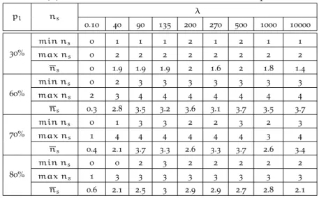
Table4.15 Shows the results for each test, wherensis the
final number of features of each subset. . . 76
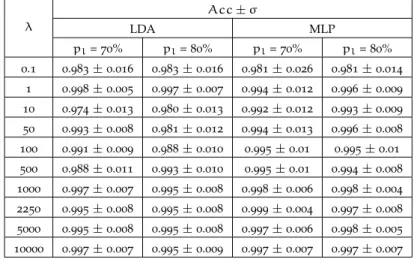
Table5.1 Average classification accuracies from models
trained with subsetΓ (with different numberns
of selected features) selected by LASSO Multi ob-jective Feature Selection method (LMFS) method
from IONO problem.nf is the original number
of features. . . 98
Table5.2 Average classification accuracies from models
trained with subsetΓ selected byLMFSmethod
from problems SONAR, PEN and ILPD. nf is
the original number of features. . . 98
Table6.1 Mean accuracy for LDA over final selected
fea-ture subset of each experiment. . . 109
L I S T O F A L G O R I T H M S
1 Basic algorithm to eliminate redundant features . . . 54 2 Basic algorithm to eliminate irrelevant features . . . 55 3 Basic algorithm for the experiments of the feature
selec-tion method based on the proposedSindex. . . 57 4 Simple pseudo-code for the Forward-Backward process. 71 5 LMFS algorithm. . . 93 6 MOBJ experiments algorithm. . . 95
A C R O N Y M S
MLP Multi Layer Perceptron
MI Mutual Information
FS Feature Selection
LASSO Least Absolute Shrinkage and Selection Operator
MOBJ Multi OBJective
LMFS LASSO Multi objective Feature Selection method
SSFC Semi-Supervised Feature selection based on Clustering
RWP Reprinted with permition from [14]
xxii list of symbols
L I S T O F S Y M B O L S
F,X original feature set
Y label output set (output variable set) Γ selected feature subset
Γℓ selected feature subset considering only labeled data
Γℓu selected feature subset considering labeled and unlabeled data nf number of features of setF
ns number of features of setΓ nn number of irrelevant features
nr number of remaining features in setFafter selecting some feature nc number of clusters
no number of outputs
nℓ number of labeled instances nt number of test instances nu number of unlabeled instances
n total number of instances (sample size) pl percentual of labeled data
nd number of crossvalidation folds np number of permutations
p number of neurons
Fi featureifrom setF Xi featureifrom setX
x sample fromX(is a vector composed by all features ofX) xi ith sample fromX(is a vector composed by all features ofX) Yi ith output variable from setY
list of symbols xxiii
Ycl cluster labels vector R relevance vector
Rc relevance vector considering cluster label information X input data set or a random discrete variable
X(ℓ) set of labeled data X(u) set of unlabeled data
ω vector of all weigths of a multi layer perceptron W vector of weigths of the output layer
Z vector of weigths of the hidden layer or a discrete random variable
Λ eigenvalues
ϑ eigenvector
H entropy
h differential entropy
H mixed entropy
MI mutual information
S similarity measure
Sp permutation ofS
A “unsupervised” term ofS B “supervised” term ofS
λ parameter to balance influence of termsAandBofS
Part I
1
I N T R O D U C T I O NRecently, due to the technological development of sensors, measure-ment systems and information storage hardware, collecting data is becoming easier and cheaper. Medical researches, as well as financial analysis, data mining and imaging are some examples of applica-tion fields that deal with, or are able to generate very large data sets. These applications have strongly demanded the development of methods that are capable to deal with new situations that appear in higher dimensions. Some problems that may arise involve dealing with redundant or irrelevant information, “curse of dimensionality” or “concentration of the euclidean norm” [96].
The analysis of higher dimensional data sets is difficult, not only because they are large in terms of number of observations, but also because of the large number of variables (features) that can be gen-erated with the new sampling engines. In fact, in most applications that we aim at, the number of features nf is much higher than the
number of observed instances (nf >> n). This is particularly true
when considering that many usual statistical methods are developed
forn >> nf under the normality assumption, what is not realistic for
the majority of real problems. Analyzing three-dimensional data is quite different from analyzing instances with thousands of features, as in gene analysis applications [21]. For such higher dimensional
space there is no way of directly visualizing the data set distribution. Moreover, for these huge number of variables it would be necessary to have an exponential number of instances (nnf) to overcome the curse of dimensionality problem. These are some reasons that explain the increasing interest in feature selection problems.
Particularly in these application fields new samples are easily gener-ated, nevertheless, labeling data can be costly and time consuming [45].
Thus, it is usual to find data sets with scarce labeled instances and a large amount of untagged input samples, like in web-based informa-tion retrieval applicainforma-tions, and in many other problems whose data sets share the same following characteristics: high dimension, few labeled instances and a large number of unlabeled ones.
In this framework, the general problem of Semi-Supervised Feature Selection (SSFS) can be characterized by the selection of a minimal and sufficient feature subset, using the labeled data setX(ℓ)={xi,yi}nℓ
i=1
and considering also the structural information implicit in the unla-beled data X(u) = {xi}ni=n
ℓ+1. In other words, the principal aim of SSFS is to solve the problem using as less variables as possible [44],
considering both labeled and unlabeled sources. Undeniably, reducing
4 introduction
the data dimensionality could help to get better understanding about the problems, allowing, in some cases, even some kind of visualiza-tion [96]. Increase in performance, reduction of computational and
measurement times, reduction of measurement costs and data storage needs are also some of the well known advantages of reducing the number of features.
In order to reduce the number of features of a data set, there are three main strategies in which, more or less, all algorithms could be classified. In the first strategy there are the so-called filter methods whose objective is to rank the features according to some supervised [58, 72] or unsupervised [106,105, 62] criterion. These methods are
fast and easy to implement. In the second strategy, the algorithms are calledWrappersand they access the accuracy of a given model in order to find the best feature subset. The third category of methods refers to the embedded algorithms. As Wrapper methods, embedded ones uses the model as part of the selection process, but perform feature selection during the training process [26,85,89].
In this thesis we approach the semi-supervised feature selection problem by two different paths. Our first approach is based on the idea of feature clustering, i.e., features that are similar should be grouped, reducing the dimension of the problem, so that redundant information is reduced. We start the development of this approach from this main idea, applying it to a simple hierarchical clustering method. We propose here a new similarity criterion that is able to consider both labeled and unlabeled data. Also we defined a stopping criterion for the feature clustering method, which is based on the statistical significance of the similarity index. A criterion to identify relevant features is also proposed taking into account the statistical significance of some relevance measure related to the target labels and the relevance of each feature in relation to the data distribution.
Still in this clustering approach we exploit the principle of homoge-neity between labels and data clusters in the development of another semi-supervised feature selection method. This principle permits the use of cluster information to improve the estimation of feature rel-evance in order to increase selection performance. We use Mutual Information in a Forward-Backward search process in order to eval-uate the relevance of each feature to the data distribution and the existent labels, in a context of few labeled and many unlabeled in-stances.
introduction 5
objective function is designed to eliminate features while solving the learning problem.
Real problems are composed of a set of discrete and continuous variables. During our research we seek in the literature for estimators of mutual information able to handle with a mixed set of variables without sucsses. Then we developed an estimator that can deal with such kind of data, and it is also presented in this thesis as another contribution.
This thesis is organized as follows. We begin by discussing about the learning and feature selection paradigms in Chapter2trying to set
a common background of the main used strategies, and introducing the principles of the semi-supervised approach, where we base our work. Then we address the Feature Selection itself in Section3, where
we try to explain the important general topics and its difference to the feature extraction task. We make a general picture of the supervised and unsupervised feature selection methods (Sections 3.1 and 3.2)
establishing their bases and then we describe the short state of art of semi-supervised feature selection in Section3.3. Then we propose
two semi-supervised feature selection methods developed during this PhD in the feature clustering approach in Section 4, and one feature
selection method proposed in the multi-objective approach in Section
5. Finally, in Chapter6we present the mutual information estimator
for a mixed set of variables.
2
L E A R N I N G A N D F E AT U R E S E L E C T I O NPA R A D I G M S
The main paradigms of machine learning are Supervised Learning (SL), Unsupervised Learning (UL) and more recently Semi-Supervised Learning (SSL). In general, when there is a labeled data set X(ℓ) =
{xi,yi}nℓ
i , withnℓobserved instances of a given problem, composed
by the input variables vector x, and by their respective output vari-able vector y(or the target concept variables), the SL schema could
be applied. The main objective of the Supervised schema is learn a supervised schema mapping function ˆy=f(x|α), whereαis the set of parameters of the
chosen model, in order to correct classify or predict the target value for any new observation. If the data set is ideally sufficient to describe the data distribution, the general function that originated the data can be found. The general scheme to perform the Supervised Learning is shown in Figure2.1.
Figure2.1: Supervised Learning Scheme.RWP
In Figure 2.1 there is a block, named DG, representing the Data
Generator, that provides the data according to a generic marginal distributionp(x). The data setX(ℓ)is sampled fromDGand delivered
to the Oracle Owhich, for each observation in this data set, knows
the target variable y. In other words, givenx, the oracle, somehow,
know the targety, so an approximation of the conditional distribution p(y|x)is known. A ModelMcan be set with the dataxand the target
variabley, in order to be used by an EstimatorEto classify or predict
the target variable y∗ for a new datax∗, given a setAof parametersα.
ModelMcan be fed with the output estimation ˆyin order to help in
the fine tuning ofαparameters.
8 learning and feature selection paradigms
If, for a given problem, there is no information about the target variable, and the only available information is a data set X(u) =
{xi}ni=n
ℓ+1 composed bynu observations of the input variables, what can be done is try to uncover the data structure. In the Unsupervised Learning schema the main goal is, broadly speaking, to estimate the densities that are like to have generated the data setX(u). As shown in
unsupervised
schema Figure2.2, the conditional probabilityp(y|x)isn’t known, i.e., there is no labeling agent in the UL scheme. Considering this, the modelMhas
to be built with sufficient ability to extract some structural information fromX(u), in order to provide to the Estimator one parametric model
to estimate the probabilityp(x∗|θ)of a new datax∗to belong or not
to one specific class (given a parameter setΘ). Roughly speaking, we
will look for clusters in this schema.
Figure2.2: Unsupervised Learning Scheme.RWP
The Semi-Supervised Learning, on the other hand, is considered to be halfway between Supervised and Unsupervised Learning. For this learning scheme, both X(ℓ) = {xi,yi}nℓ
i and X(u) = {xi}ni=nℓ+1 data sets are available, and the objective is try to use them, in some way, to build the model. The SSL can be performed within two different per-semi-supervised
schema spectives: in the Supervised Learning Perspective where the learning task is executed in a supervised scheme with additional structural in-formation inferred fromX(u)∪X(ℓ); or in the Unsupervised Learning
Perspective, where the learning task is performed in an unsupervised scheme with side constraints.
The general scheme for the SSL schema with the supervised per-spective is shown in Figure 2.3. This scheme is basically the same
for the SL one adding some information from the unsupervised data. The datax∈X(ℓ), for which the target variablesyare known by the
labeling agentO, is drawn fromDGand provided, together with the
label information, to the modelMss. This modelMssdiffers from the
learning and feature selection paradigms 9
probability density estimated by the estimatorEu. This estimator, in
turn, was tuned by the unsupervised modelMu. By the way, theMu
model works together with the datax∈X(u), whose output variable
values are not known by the Oracle, and, of course, with the data from
X(ℓ), both drawn byDGfrom the same distribution.
Figure2.3: Semi-Supervised Learning Scheme within the Supervised
Per-spective.RWP
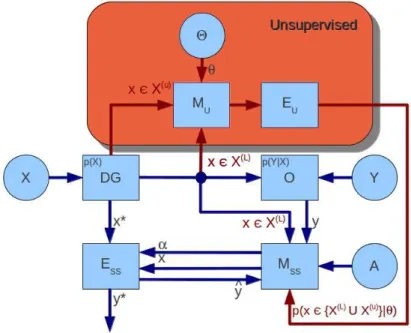
Figure2.4shows the scheme for the SSL under an Unsupervised
Perspective. The approach for this perspective is based on the Unsu-pervised Learning scheme, adding the labeling agent to handle with the part of data whose target variables are known. Then, the modelM
has to provide some probability density inferred from the input data densities with support of the labeled data. In other words, the search for natural clusters in the data has to be consistent with the labeled data.
There are a lot of real problems where do not exist only labeled data. For example, just to mention a very simple one, every day a lot of web pages are created and stored in the internet and not properly classified or indexed. So, problems like data mining in the internet count with a huge unlabeled data set (not classified web pages). It is important to notice that these unlabeled data sets are usually huge when compared to the labeled data set, i.e. the number of unlabeled instances is much bigger than the number of instances of the labeled data set (nu >> nℓ).
obser-10 learning and feature selection paradigms
Figure2.4: Semi-Supervised Learning Scheme within the Unsupervised
Per-spective.RWP
vations, that they are not sufficient to represent the class-condition densities (undersampling), favoring the occurrence of problems as biased sampling. This means that these few samples may have been obtained by a very specific condition, so, they are biased by this con-dition, for example, in the case of on-line polls. Individuals that have more strong convictions are more likely to fill the poll rather than persons with weak convictions about the subject. This fact could be even worse if the assumption of i.i.d. of the data is not meet, then, having more information should be interesting. In that sense, if there are a lot of data, even unlabeled, probably it is possible to get some useful structural information from data distribution, which could be used in order to increase the model accuracy. In other words, as the learning problem may not be completely specified by X(ℓ), maybe,
prior information (or assumptions) will be needed, and, the knowl-edge about p(x|θ) should improve the estimation of p(y|x). That is
why the Semi-supervised approach is used in the learning task. Together with all these problems, frequently, the learning task is faced with another important detail: in many problems, not only the small number of labeled instances is the main problem, but also the number of variables. Nowadays, with the advance of technologies, high dimensional
problems like microarrays analyses in the bio-informatics field for example, the number of variables could reach thousands, or even tens of thousands. In theory, dealing with large number of features, especially when it is larger than the number of instances (nf >> nℓ), is possible,
learning and feature selection paradigms 11
dimensionality” [96], “concentration of measure phenomenon” [96]
and overfitting have to be taken into account. Of course, as the required size of the labeled data set, in order to assure good representation of the data densities, is not met, two actions could be taken in order to avoid or minimize these problems:
• label new instances: but labeling data is, in general, very costly and time demanding. It would be nice, however, by definition, this is not a feasible solution;
• reduce the number of variables: if we succeed in finding redun-dant or irrelevant features we can eliminate them and reduce the dimension of the data set.
So, feature selection seems to be a good way to deal with these problems. In order to have a broader view of the problem that we want to address, we will formally start defining its scope. We are interested in dealing with databases characterized by a large number
nf of features, a small numbernℓof labeled instances and by a high
number nu of unlabeled samples. The data set X = X(ℓ)∪X(u) problem definition is defined by the union of the labeled data set X(ℓ) = {xi,yi}nℓ
i and
the unlabeled data set X(u) = {xi}n
i=nℓ+1 where each instance is de-fined as a vector xi = {xi,1,xi,2,. . .,xi,nf} where nf is the number of features, and the labels or target variables are defined as a vector
yi={yi,1,yi,2,. . .,yi,no}beingno the number of target variables. In our case, for simplicity we will consider only one output variable thenyiwill be the class label or the target value for instancexiin the
labeled data set. Finally, lets define that the data setXhasnu >> nℓ
andnf>> nℓ+nu.
Performing feature selection in a data set with a small number of labeled instances, whose number of features are huge, tends to fail if done in a Supervised scheme. For example, the relevance of a feature can be measured by its correlation with the target variable and, when evaluated in a data set too small, features that seems to be very relevant, could not be at all. On the other hand, unsupervised methods do not take into account the labeled information, which are few but important. As the problem may not be completely specified byX(ℓ)orX(u) separately, maybe, considering theX(ℓ)data set with
some additional information from unlabeled data setX(u)could help
the feature selection task.
Lets define the set F = f1,f2,. . .,fj nf
j=1 of all features, where
each featurefj=fj,1,fj,2,. . .,fj,i
nℓ+nu
i=1 is a vector composed by the
values of featurejof all instances. The selection of a minimal feature
subset Γ, where Γ ⊆ F, which is necessary and sufficient to induce
12 learning and feature selection paradigms
In the same way that was defined before for the Semi-Supervised Learning, in this selectionscheme, both X(ℓ) = {xi,yi}nℓ
i and X(u) =
{xi}ni=n
ℓ+1 data sets are available, and the objective is try to use them, in some way, to build the model. The Semi-Supervised Feature Selec-tion schema (SSFS) also can be performed within the two different perspectives: within asupervised perspectiveor within anunsupervised perspective.
The general scheme for the SSFS with the supervised perspective is shown in Figure2.5. This scheme is basically the same shown for the
SSL one, but here, the so-calledMssmodel has also the capability to
select features. Likewise in the SSL, the datax∈X(ℓ), with marginal
semi-supervised FS
schema distribution p(x), and whose target variables Y are known by the labeling agentO, is drawn from the Data GeneratorDGand provided,
as well as the label information, to the modelMssfs. This model is
able to use some informationΨinferred fromXby the unsupervised
model Mufs, which in turn, was tuned by a given parameter set Θ.
TheMufs model works withx∈ Xdrawn byDGwithout the need
of known the output variable values. A subset Γ is defined byMssfs
and given to a specific learning modelMin order to predict the target
variable or classify the data, for any new instancex∗. The modelMssfs
may need to access the accuracy of the modelMif it is a wrapper or a
embedding method.
Figure2.5: Semi-Supervised Feature Selection Scheme within the Supervised
Perspective.RWP
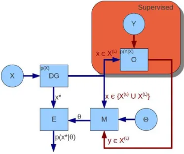
Figure2.6 shows the scheme for the SSFS under theunsupervised
perspective. Basically, the modelMufs, given a parameter setΘtries to
select features based on the data densities over all instances inXand
using the label information given by the labeling agentOfor the part
learning and feature selection paradigms 13
Figure2.6: Semi-Supervised Feature Selection Scheme within the
Unsuper-vised Perspective.RWP
3
S TAT E - O F - T H E - A RTFeature Selection is a topic whose importance is growing enormously lately, especially in fields like medical research, financial analysis, data mining and imaging, just to cite a few ones. There is a wide range of applications in these and other fields, like EEG recordings and gene analysis which have, among their most important objectives, the attempt to better understand the pathologies and, obviously, find more adequate treatments. Analysis of financial time series by the stock market agents and the consumer behavior by credit card companies are also applications that deal or produce huge data sets and have been strongly demanding the utilization of tools to “select the features” that are more relevant for their analysis.
The principal aim of feature selection is to solve a problem using as few variables as possible [44], either for data mining, function
approximation or identification.
The fact that the means for collecting data are becoming more easy and cheap, coupled with the very need to understand the problems and find solutions, like in medical researches using gene expressions of cancer tumors for example, produces incredibly large databases.
However, just collect as much data as possible does not means that dimension reduction it will be more easy to solve the problems. Intuitively we are led
to think that more information is better than less information, but having a lot of data does not mean that we have the right information. Then, problems related to the increase of the space dimensionality, like redundant or irrelevant information, the “curse of dimensionality” or the “concentration of the Euclidean norm” [96] arise and have
to be considered in order to be successful when dealing with such databases.
It is difficult to analyze these databases because they are large in terms of the number of observations, and because of the large number of variables. It is very different to analyze one hundred observations of three-dimensional data, whose data can be visualized in a three dimensional graph, from analyzing one hundred instances with
thou-sands of features, as is the case in gene analyses applications. For such high dimensional issues
large number of variables it would be necessary nearnnf instances to overcome the curse of dimensionality problem. Especially considering that many classical analysis tools are developed for n >> nf and
under the assumption that data is normally distributed, which is not usually true in real problems. In these cases feature selection is a way to overcome all these difficulties.
16 state-of-the-art
Nevertheless, there is another specific characteristic of these large databases that has to be considered. It is not so easy to collect data that are associated to the output variables or to the target concepts, for a given problem, because labeling data is costly and time consuming [45].
Therefore it is usual to find data sets composed with more unlabeled data than labeled data. In the data mining domain, for example, when scarce labeled data
someone types some words in the search engine of his browser, he want to receive a list of “all” pages related to that subject. However, there are thousands or even millions of web pages on the internet, without any proper index or classification about their contents. Of course the search mechanism, in order to return to the user the list of web pages most related to a specific subject, can deal only with some well indexed web pages, but this would reduce drastically the search space. One good idea is try to get some information from the large number of non-indexed web pages. The feature selection performed in such way, using labeled and unlabeled data, is called Semi-Supervised Feature Selection (SSFS) and this concept will be better explained in Section3.3. Like in this example, there are a lot
of problems sharing the same characteristics: high dimension, few labeled instances and a lot of unlabeled ones. The challenge is to use some structural information from the labeled and unlabeled instances in order to improve the solutions.
To reduce the number of features of a data set, there are three general strategies where, more or less, algorithms could be classified. In the first strategy there are the so-called filter methods whose objective is to rank the features according to some relation (or correlation)[58,72]
between the input variables and the target concepts [106, 105, 62].
These methods are fast and easy to implement, but, filters that use a feature selection
strategies univariate index, in general, fail in considering the relevance of a given feature in the presence of other features [44]. In the second strategy,
the algorithms are called wrappers and they access the accuracy of a given model in order to find the best feature subset. Technically they are the best approach, but they usually have to perfor an exhaustive search over all possible subsets of features which is costly and, even for problems with relatively small dimension, unfeasible. The third category of methods refers to the embedded algorithms. As Wrapper methods, embedded ones uses the model as part of the selection process, but perform feature selection during the training process [26, 85,89].
The feature selection task can be also classified into three distinct categories according to the type of available data. This classification was explained in details at item2and here we limit ourselves to list
them with a brief resume of their characteristics:
state-of-the-art 17
• Unsupervised Feature Selection: the data has no labels or target feature selection categories variables, and the selection task has to be done in a unsupervised
scheme;
• Semi-Supervised Feature Selection: there are both labeled and unlabeled data available to perform the task.
Many methods of each one of these categories can be implemented in, at least, two basic search strategies namedForward Selectionor Back-ward Elimination. In the forward feature selection the algorithms begin with an empty set of features and go on adding relevant variables, given previously selected variables. This strategy has smaller capabil-ity to finding more complementary features, compared to backward feature selection, because it starts within a context of none selected feature. In the other hand even the smallest nested subset is predictive. This last characteristic is more interesting when dealing with the trade performance for number of features. The backward elimination begins with a set of all features and goes on eliminating irrelevant variables, given the remaining selected variables. This method is capable of finding complementary features, because it start its analysis with all features, however, its performance is degraded for smallest nested subsets [42].
feature selection versus feature extraction
The termfeature extractionhas a different meaning fromfeature selection. They are different in the sense that the second one selects a reduced subset from the set composed by all features, while the first one aims to construct a second smaller set of variables, using all features from the original set. In the literature there are a lot of methods that perform feature extraction and some of them are very popular as Principal Component Analysis (PCA) or ISOMAP.
The PCA [56] method transforms the data to a new coordinate
system in which the greatest variance of projected data will be the first
coordinate. The ISOMAP [88] method tries to discover the manifold feature extraction methods
structure generating a mapping that preserves the geodesic structure. Other methods that perform feature extraction also can be cited, as Locally Linear Embedding (LLE) [78], Laplacian Eigenmaps [9], a
linear method called Locality Preserving Projections [50] (LPP) and
a method that tries to find the low-dimensional representation of each data point, looking for a function that minimizes the error when reconstructing the high-dimensional data point representation [104].
Another well known method is the supervised Linear Discriminant Analysis one (LDA) [32], which calculates projection vectors in order
to maximize the between-class-variance and minimize the within-class-variance of projected data points. In [2] the authors extend this
Dis-18 state-of-the-art
criminant Analysis), whose objective is to find a projection, respecting semi-supervised
feature extraction
methods the discriminant structure inferred from labeled data, and respectingthe intrinsic geometrical structure inferred from both labeled and
unlabeled data. The labeled data is used to maximize the separabil-ity between classes, and the unlabeled data is used to estimate the intrinsic geometrical structure of the data.
In [103] the authors proposed the so called SSDR algorithm
(Semi-supervised Dimensionality Reduction). This method tries to preserve in the projected low-dimensional space, the structure of original data space (with high-dimension) and the pairwise constraints previously defined. It exploit themust-linksandcannot-linksconstraints together with unlabeled data. Its motivation using unlabeled data is enhance performance and stability when constraints are few.
Hou et. al. in [54] extend the Semi-supervised Dimension Reduction
method [103] cited before, in order to use multiple representation
forms of data, employing the domain knowledge in the form of pair-wise constraints.
Alternatively, in [101] the authors tries to use some prior information
to improve the stability of solutions, withal, they show that in the case of LLE and Local Tangent Space Alignment methods the prior information only helps in limiting the freedom of translation and scaling, and, when applying to ISOMAP method, it does not result in any important improvement.
All these methods, somehow, tries to project the data into a new feature space with reduced dimension, nevertheless, in this thesis we are interested in deal with theFeature Selectiontask, instead ofFeature Extraction.
In the literature there are a lot of methods that perform Feature Selection in a supervised and in a unsupervised way. In this section we intend to present some of them, trying to explain their main ideas and assumptions before introducing properly the state of art of the semi-supervised feature selection. It is important not only know the existing methods related to the semi-supervised feature selection task, but also to search for ideas in the purely supervised and unsupervised methods in order to get some good insights to our goal.
3.1 supervised feature selection
3.1 supervised feature selection 19
Pearson based method
We start with one classical individual relevance index that is very
simple and well known, thePearson correlation coefficient[71]. This Pearson coefficient coefficient is shown by equation3.1:
C(j) =
Pn
i=1 xi,j−xj¯
(yi−y¯) q
Pn
i=1 xi,j−xj¯ 2Pn
i=1(yi−y¯)
2 , (3.1)
where n is the number of instances, Xj is the vector containing all
instances of thejth feature,xi,jis theithinstance ofXj,yis the vector
containing the target values and the bar notation means average over theielements ofXj.
This very simple linear method is a univariate one, because it makes independence assumptions between features. The features are ranked according to their coefficients, with a low computational and statistical complexity. It has a linear computational cost with respect to the num-ber of features and instances. Nevertheless, the fact of not considering the effect of the iterations among features is its drawback, because single features that do not have any relevance, can be extremely useful when considered in the presence of others! This constitutes the main reason that why we do not use this coefficient in the development of our methods.
Gram-Schmidt based methods
The Gram-Schmidt orthogonalization procedure [6] can be applied
in a method to select features. It is a linear multivariate and selects variables by adding progressively variables, which correlate to the target, in the space orthogonal to the variables already selected.
In the work of Oukhellou et. al. [69], a version of Gram-Schmidt
orthogonalization procedure is used to iteratively rank the features. In Gram-Schmidt a first step the relevance of each feature is determined measuring the
20 state-of-the-art
method as explained before. At the end, all features ranked below the random feature are considered irrelevant and discarded. However, it is necessary to generate a lot of random descriptors to make a good estimation of the cumulative distribution function of its rank.
This last criterion is applied in another work [85] in a slightly
different way. The Gram-Schmidt method is also used to rank features, but in this case a new procedure to stop selection and to select the best ranked features was developed. The idea is not to rank all features and to select a threshold, but to stop the process at any point. The criterion is also based on the cumulative distribution function of the rank position of a random probe added to the initial feature set. It states that since the probe is a random variable, its rank position is also a random variable. At each step of Gram-Schmidt method the features are orthogonalized, and then the feature with smallest angle value related to projected output vector is selected. The cumulative distribution value is then evaluated and if this value is smaller than a defined risk this feature is definitely selected and the next step of Gram-Schmidt can be performed. Otherwise the process is stopped. This risk is defined as being the probability of the selected feature be less significant than a random one (probe).
Recursive Feature Elimination Support Vector Machine algorithm
TheRecursive Feature Elimination Support Vector Machine algorithm (RFE-SVM) [43] is an example of a backward elimination wrapper method.
The idea is very simple: a SVM is trained and then, the feature with smallest weight in absolute value is discarded. Then the model is RFE-SVM
trained again without this feature and the process continues recur-sively until the desired number of selected features is reached. Of course, this method has a expensive computational cost that could be a little less if more than one feature is discarded at each iteration, how-ever, it can compromise the optimality of the result. This multivariate method can be extended to the non-linear case too.
RELIEF based methods
Feature Selection, by definition, is the problem of selecting one small feature subset which is “ideally, sufficient and necessary” [58] to
3.1 supervised feature selection 21
The supervised RELIEF method was first proposed by Kira et al. [58],
and its main propose was to avoid the problem of an exhaustive search in a Feature Selection framework, or even prescind from choosing an heuristic strategy to this search. It is a non-linear feature ranking filter.
RELIEF is based on the maximal margin concept, so, the weight calculated for one feature will be as high as discriminative this feature
could be. Roughly speaking, this method takes for each instance in RELIEF the training set, the nearest neighbor from the same class (Near Hit)
and the nearest neighbor from the other class (Near Miss). There-fore the distance1 between each instance and its near hit and near miss neighbors, for each feature, is evaluated. The Relevance value assigned to each feature will be the sum of the difference between these two distances over all instances. The far from each other, along the axis defined by the considered feature, are these differences for each instance, the more discriminative is this feature and the larger is its weight. Finally the selected features will be those whose relevance values are higher than a given threshold.
It is important to highlight that RELIEF only works well if the relevance values of the relevant features are sufficiently larger than those of the irrelevant features, and, of course, if a threshold can be defined to split them. However, these are not the only problems for RELIEF. As the search is performed assigning weights to each feature instead of selecting subsets, these weights can be thought as a space mapping, therefore, the features in the original data space are being mapped into a new feature space that we will callinduced feature space. The problem here is that two instances that are close in the original feature space, may not be, in the induced feature space. Another important problem is concerning the margin definition: the margin is calculated as an average margin and any outliers will have
a high influence over its value. Then, the I-RELIEF [86] was developed I-RELIEF based on RELIEF in the attempt to avoid these problems, being able
to handle with large data sets.
The main idea of I-RELIEF, to overcome these issues, is to compute the margin in the “induced” feature space. But in this case, the weights are not known before learning, so the solution was developed one probabilistic model where the neighbors are treated as “latent vari-ables”. The margin defined in terms of this probabilistic model takes into account the probability of neighbor of an instance belonging to the same class of another one or not. See [86] for details.
This last method (I-RELIEF), was extended to the semi-supervised case in [62], considering the margin of the unlabeled data (large
margin principle) in the objective function of the Logistic I-Relief method presented in [86]. This semi-supervised method is detailed in
Section3.3.
22 state-of-the-art
Optimal Brain Damage
The central idea of OBD method [26] (Optimal Brain Damage) is to
determine, in a neural network, which are the connections (weights) to be pruned first using the saliencyvalue. The saliency measures how important is one parameter in relation to the output of the network, or, in other words, which are the weights, that when deleted, less affects the training error. Basically, one has to train a network, evaluate OBD
the saliency values of each weight, and discard the one with the smallest saliency value. In this work the saliency of each network parameter is evaluated using one meaning justified formula, and not just considering the magnitude weights as a measure of the saliency. See [26] for more details. The procedure is recursively performed
until a stopping criterion is reached. OBD is an example of backward elimination embedded method. It is non-linear and, as all variables are considered together in the calculations, it is a multivariate method.
Mutual Information based methods
In [61] the authors propose a very simple supervised method to select
the important features using the mutual information as a similarity measure. Similar features are clustered in an hierarchical way and after the clustering step, the relevance of each cluster to the output is evaluated within a forward procedure. The Mutual Information (MI)
evaluated between the features is used to evaluate the redundancy in the first step and theMIbetween the features and the output variable
is used to evaluate their relevance in the next step. There is one slight detail in the way that they apply the hierarchical method: here only consecutive features could be clustered because the method was being applied to a frequency spectral data. The clustered features are then replaced by a mean feature. For further information please refer to [61].
Another method based onMIto select features was developed by
MI based methods
François et al. [35]. It uses the permutation test to set a threshold
for the mutual information between each variable to the output and therefore select those features whose MI value is greater than this
limit. The permutation test is also used in [92,28] to find statistically
significant relevant and redundant features by means of filters using mutual information between regression and target variables. After that, good candidate feature subsets are searched by a wrapper, taking into account the regression model. This is an hybrid filter/wrapper features selection algorithm.
. . .
3.2 unsupervised feature selection 23
however, a very good review on these supervised methods and feature selection can be found in [44].
3.2 unsupervised feature selection
Given the nature of the problems that we want to address, and the fact that we have to deal with a lot of unlabeled data, we decided to give an special attention to the unsupervised feature selection methods. Maybe, we can get some good ideas in order to develop our method and achieve our goals. These methods have some interesting advantages and among then we can highlight that they are unbiased by any experimental expert, they perform well in the absence of any a priori knowledge and reduce the overfitting risk. Nevertheless, their main drawback is that they rely on some mathematical principles with no guarantee that it will work for any kind of problems. These feature selection methods are based on a unsupervised paradigm which can be derived from the general scheme to perform the unsupervised learning as explained in Section 2 schematized in Figure 2.2. We
found some interesting unsupervised methods in the literature and the following paragraphs are dedicated to their presentation.
KNN based method
The first method to be presented is a KNN based one which performs feature selection using feature similarity. In [68] the authors propose
a new metric called maximum information compression index(MICI) to
be used in the algorithm. This new metric is defined as the smallest KNN eigenvalue of the covariance matrix evaluated for any two random
variables
The value of MICI is zero when features are linearly dependent indicating that these two features are very similar and can be grouped. Basically, the algorithm selects the most compact feature set, i.e. the cluster of neighbors of each variable which has the smallest distance to its kth neighbor is selected. Then, all k nearest features of the
selected cluster are discarded, and process is repeated until all features have been selected or discarded. This method is very sensitive to the parameterkand adjusting this value is not a simple task. Please refer
to [68] for a detailed explanation.
SVD-entropy based method
One very interesting idea is shown in [95]. In this work the authors