Detection of ground fog in mountainous areas from MODIS day-time data using a statistical approach

(1)

AMTD

8, 12155–12201, 2015

Detection of ground fog in mountainous

areas

H. M. Schulz et al.

Title Page

Abstract Introduction

Conclusions References

Tables Figures

◭ ◮

Back Close

Full Screen / Esc

Printer-friendly Version Interactive Discussion

Discussion

P

a

per

|

Discussion

P

a

per

|

Discussion

P

a

per

|

Discussion

P

a

per

|

Atmos. Meas. Tech. Discuss., 8, 12155–12201, 2015 www.atmos-meas-tech-discuss.net/8/12155/2015/ doi:10.5194/amtd-8-12155-2015

This discussion paper is/has been under review for the journal Atmospheric Measurement Techniques (AMT). Please refer to the corresponding final paper in AMT if available.

Detection of ground fog in mountainous

areas from MODIS day-time data using

a statistical approach

H. M. Schulz1, B. Thies1, S.-C. Chang2, and J. Bendix1

1

Laboratory for Climatology and Remote Sensing, Faculty of Geography, Philipps University, Marburg, Germany

2

Department of Natural Resources and Environmental Studies, National Dong Hwa University, Hualien, Taiwan

Received: 22 October 2015 – Accepted: 10 November 2015 – Published: 20 November 2015

Correspondence to: H. M. Schulz (martin.schulz@geo.uni-marburg.de)

(2)

AMTD

8, 12155–12201, 2015

areas

H. M. Schulz et al.

Title Page

Tables Figures

◭ ◮

Back Close

Full Screen / Esc

Discussion

P

a

per

|

Discussion

P

a

per

|

Discussion

P

a

per

|

Discussion

P

a

per

|

Abstract

The mountain cloud forest of Taiwan can be delimited from other forest types using a map of the ground fog frequency. In order to create such a frequency map from re-motely sensed data, an algorithm able to detect ground fog is necessary. Common techniques for ground fog detection based on weather satellite data can not be applied

5

to fog occurrences in Taiwan as they rely on several assumptions regarding cloud prop-erties. Therefore a new statistical method for the detection of ground fog from MODIS data in mountainous terrain is presented. Due to the sharpening of input data using MODIS bands 1 and 2 the method provides fog masks in a resolution of 250 m per pixel. The new technique is based on negative correlations between optical thickness

10

and terrain height that can be observed if a cloud that is relatively plane-parallel is trun-cated by the terrain. A validation of the new technique using camera data has shown that the quality of fog detection is comparable to that of another modern fog detection scheme developed and validated for the temperate zones. The method is particularly applicable to optically thinner water clouds. Beyond a cloud optical thickness of≈40,

15

classification errors significantly increase.

1 Introduction

Cloud forests are a tropical and subtropical forest type ecosystem characterized by the frequent occurrence of ground fog conditions (Bruijnzeel et al., 2010). As they intercept water from cloud droplets and, due to their mostly wet canopy, have a decreased rate of

20

transpiration, they play an important role as an ecosystem service provider increasing local water supplies (Mildenberger et al., 2009). Furthermore they are biodiversity hot spots with a high number of endemic species (Postel et al., 2005). This also holds true for the cloud forest of Taiwan (Hsieh, 2002). While cloud forest areas of Taiwan are already the subject of intensive research (cf. e.g. Mildenberger et al., 2009; Chu

25

(3)

country-AMTD

8, 12155–12201, 2015

areas

H. M. Schulz et al.

Title Page

Tables Figures

◭ ◮

Back Close

Full Screen / Esc

Discussion

P

a

per

|

Discussion

P

a

per

|

Discussion

P

a

per

|

Discussion

P

a

per

|

wide scale. The most comprehensive information about the extent of cloud forest in Taiwan available today is given by Li et al. (2013), based on the National Vegetation Database of Taiwan. Since this data is based on field surveys it is of high reliability but it only does cover the area of 9822 plots (each with an area of 400–2000 m2) distributed over the whole country. Due to the inaccessibility of Taiwan’s mountainous areas, those

5

plots are mainly located close to roads.

For a spatial-explicit mapping, the usage of remote sensing data seems advisable. As the occurrence of cloud forest depends on the heavy influence of ground fog con-ditions, it has been shown by Mulligan and Burke (2006) that it can be discriminated from other forest types by the application of a threshold on maps of the ground fog

fre-10

quency. The potential of this approach for the application in Taiwan has been shown by Thies et al. (2015) using low stratus frequency maps derived from Moderate-resolution Imaging Spectroradiometer (MODIS) data. Because no distinction has been made in this study between low stratus clouds (including clouds without ground contact) and ground fog, the explanatory power of the presented low stratus frequency maps is,

15

however, limited. To obtain more significant ground frequency maps, an algorithm able to detect ground fog (defined here as any cloud with ground contact) in Taiwan from satellite data is necessary. Common techniques for ground fog detection are analysed with respect to their applicability for Taiwan in Sect. 2.1. A new method which is more suitable for mountainous areas is presented in Sect. 2.2.

20

2 A ground fog detection approach suited for Taiwan

2.1 Existing approaches

In order to detect ground fog from space, commonly a plane cloud base is assumed. The height of the cloud base is compared to a digital elevation model (DEM). If it is equal to or below the terrain height taken from the DEM, ground fog conditions can be

25

(4)

AMTD

8, 12155–12201, 2015

areas

H. M. Schulz et al.

Title Page

Tables Figures

◭ ◮

Back Close

Full Screen / Esc

Discussion

P

a

per

|

Discussion

P

a

per

|

Discussion

P

a

per

|

Discussion

P

a

per

|

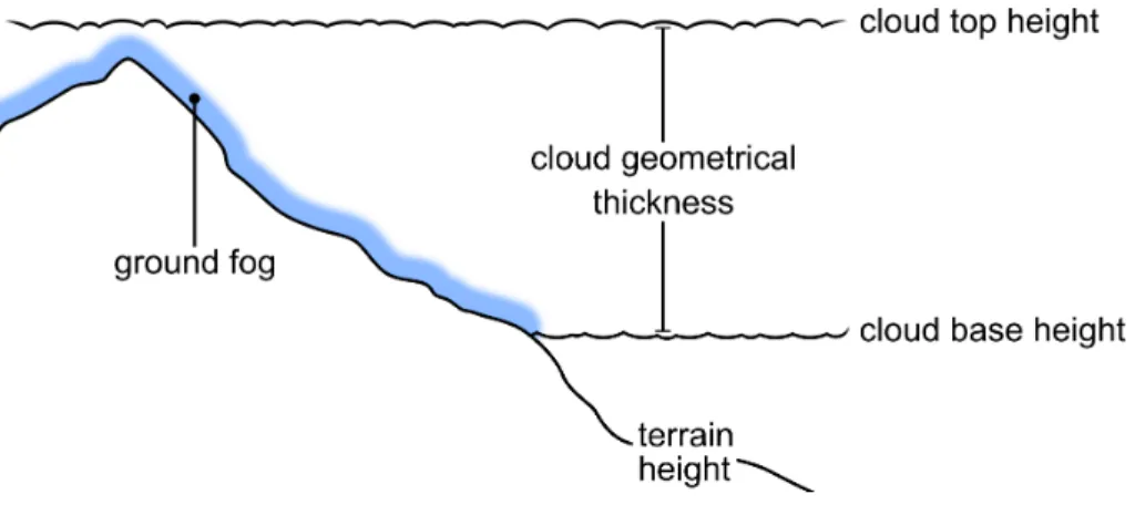
the lifting condensation level of clouds (the area of which is taken from High-resolution Infrared Radiation Sounder HIRS data) from monthly WorldClim data that is interpo-lated from station measurements (Hijmans et al., 2005). For a higher temporal resolu-tion and a more precise cloud base, usually the height of the cloud top and the cloud geometrical thickness are retrieved from satellite data using the abstraction of a

plane-5

parallel cloud geometry (not to be confused with plane-parallel cloud models as they are used in radiative transfer calculations). This is possible as ground fog conditions are commonly caused by stratiform clouds. The height of the cloud base can then be calculated by subtracting the cloud geometrical thickness from the cloud top height (cf. Fig. 1).

10

Di_fferent methods for the cloud top height retrieval as e.g. CO₂slicing (Menzel et al., 1983), DEM extraction (Bendix and Bachmann, 1993) or a method recently presented by Yi et al. (2015) do exist. As they are not suited for low clouds or do only work under certain conditions, they cause di_fferent problems if the aim is to apply them in ground fog detection over mountainous areas (cf. Table 1). Cloud top heights may also be

15

calculated from the cloud top temperature retrieved from infrared window channels. Cermak and Bendix (2008) compare it to the temperature of surrounding land pixels. Under the assumption of a certain (negative) temperature lapse rate with altitude the height of the cloud top above ground can then be calculated. Besides the problem that the assumed temperature lapse rate may not be given in many cases, this approach is

20

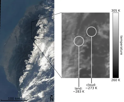
neglecting material properties such as albedo or heat capacity and therefore the diff er-ent reactions of cloud and ground pixels to illumination or temperature changes. It has, however, been successfully tested in the temperate zones of the Earth (Cermak and Bendix, 2011) so that these problems seem not to be crucial in general. In Taiwan the situation seems to be different, as shown in a MODIS scene containing ground fog in

25

(5)

AMTD

8, 12155–12201, 2015

areas

H. M. Schulz et al.

Title Page

Tables Figures

◭ ◮

Back Close

Full Screen / Esc

Discussion

P

a

per

|

Discussion

P

a

per

|

Discussion

P

a

per

|

Discussion

P

a

per

|

difference between the fog and the land surface is about 10 K, which would result in a height difference of at least several hundreds of meters if a reasonable lapse rate is assumed.

Different methods are also available for cloud geometrical thickness derivation (cf. Table 2). Simple approaches that use empirically derived relationships between the

5

thickness and the liquid water path (LWP) of a cloud (Hutchinson, 2002) or its optical thickness (Minnis et al., 1997) lack precision because of oversimplification. More so-phisticated approaches applied in ground fog detection schemes as pseudosounding (cf. eg. Chang and Li, 2002; Bendix et al., 2005) or an approach based on iteratively simulated LWPs used by Cermak and Bendix (2008) use more complex cloud

parame-10

terizations but do rely on many assumptions regarding cloud microphysical properties and their vertical distribution within the cloud. These assumptions may be valid for ra-diation fog. The typical Taiwanese mountain fog, however, seems to be – based on field experience and information given by Li et al. (2015) – more of advective nature. While it has not been tested if existing cloud thickness retrievals can be applied despite

15

some inaccuracies, the main problem of an accurate cloud top height derivation would remain.

2.2 The new approach – theoretical preliminary considerations

The main problem in ground fog detection in Taiwan is the derivation of cloud top heights. A method that does not take this intermediate step and detects the cloud

20

base directly instead seems to be suited to overcome it.

For an assumed plane-parallel cloud as shown in Fig. 1 the geometrical thickness is by definition the same for all parts of the cloud that do not touch the terrain. If that cloud is, however, cut o_ffby the terrain in some parts (causing ground fog), its thickness would be reduced in this area. If it is additionally assumed that the cloud is horizontally

ho-25

(6)

(de-AMTD

8, 12155–12201, 2015

areas

H. M. Schulz et al.

Title Page

Tables Figures

◭ ◮

Back Close

Full Screen / Esc

Discussion

P

a

per

|

Discussion

P

a

per

|

Discussion

P

a

per

|

Discussion

P

a

per

|

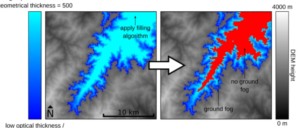
creasing with an increasing height of the terrain). For such an assumed cloud, a simple filling algorithm could be applied on an image of its optical thickness in order to flag all the pixels with the same values (cf. Fig. 3). In the flagged pixels the cloud would not have ground contact (red, right side). The unmarked cloud pixels (shades of blue, right side) would have ground contact causing ground fog.

5

A real-world stratiform cloud is neither perfectly plane-parallel nor horizontally homo-geneous in its optical properties. It can be described by this model only to some degree. Therefore a simple filling approach is obviously not suitable for fog detection. The pixels without ground contact would still have different optical thickness values. It can, how-ever, be assumed that no statistical relationship between the height of the terrain and

10

the optical thickness is given in the parts of the cloud that are not touching the ground. In contrast, there is a negative correlation between the terrain height and the optical thickness for the pixels with ground fog as the geometrical thickness decreases with increasing terrain height. Without knowledge about the vertical distribution of a cloud’s extinction coefficient a linear correlation can not be assumed. It is only known that the

15

optical thickness decreases with increasing DEM height. Such a trend can be detected using Spearman’s rank correlation coe_fficient (ρ).

Let ρ_below_h be Spearman’s rank correlation coefficient calculated from the DEM

height and the remote sensed optical thickness of all pixels of a cloud entity with a DEM height below a certain height h. If we assume perfect conditions (a perfectly

20

plane-parallel cloud without any horizontal inhomogeneities and a perfectly retrieved – no sensor noise etc. – optical thickness),ρ_below_h should be 0 for allhat the level of or below the cloud base height. For allhabove the cloud base height it should be below 0 and decrease with increasingh. Letρ_above_h be the correlation between height and op-tical thickness calculated from all cloud pixels with a height above or equal toh. Under

25

perfect conditionsρ_above_hshould be−1 for allhat the level of or above the cloud base height. For allhbelow the cloud base height it should be above−1 and increase with decreasingh. Based on this, the height in which the differenceρ_di_ff_h₌ρ_below_h−ρ_above_h

(7)

AMTD

8, 12155–12201, 2015

areas

H. M. Schulz et al.

Title Page

Tables Figures

◭ ◮

Back Close

Full Screen / Esc

Discussion

P

a

per

|

Discussion

P

a

per

|

Discussion

P

a

per

|

Discussion

P

a

per

|

As Fig. 4 shows, this theoretically assumed relation between optical thickness and terrain height can be observed for real clouds with ground contact. Above the measured cloud base height the optical thickness decreases with the height of the DEM as the cloud is cut offby the terrain here. Below the cloud base height, no relationship between optical thickness and DEM can be observed. In this real-world example,ρ_{above cloud base}

5

does, of course, not reach values as extreme as −1 and also ρ_{below cloud base} is not exactly 0.

The domain of the scatter plot in Fig. 4 has been chosen relatively small on purpose. Further in the North – where the DEM values are decreasing – also the optical thick-ness decreases. The assumption of plane-parallelism and/or horizontal homogeneity

10

thus is clearly not valid for the depicted cloud. On a more local level, however, the variability of cloud top height, cloud bottom height as well as the coe_fficient of extinc-tion is negligible. Therefore the correlaextinc-tions necessary for cloud base detecextinc-tion should be calculated for each cloud pixel p separately based only on the cloud pixels inside a round moving window centred at each p. This should be done for all pixels that are

15

according to the DEM below p (resulting inρ_{below p}) as well as for all pixels at the height of or above p (ρ_{above p}) resulting in the differenceρ_di_ff_p₌ρ_{below p}−ρ_{above p}. Withρ_{above p}

including p itself, the value ofρ_di_ff_p is, according to the above considerations, espe-cially high for pixels that are the lowest that still are located above the local cloud base height. This is becauseρ_{above p}is clearly negative here whileρ_{below p}is close to 0 (cf.

20

Fig. 5). Pixels with a local maximum ofρ_di_ff_pand clearly negative values ofρ_{above p}can therefore be considered as being most likely cloud base height pixels.

The new algorithm for ground fog detection making use of the theoretical basis de-veloped in this section is presented in detail in Sect. 4.1 and is validated in Sect. 4.2. As all of the above consideration rely on clouds being cut offby mountains, its application

25

(8)

AMTD

8, 12155–12201, 2015

areas

H. M. Schulz et al.

Title Page

Tables Figures

◭ ◮

Back Close

Full Screen / Esc

Discussion

P

a

per

|

Discussion

P

a

per

|

Discussion

P

a

per

|

Discussion

P

a

per

|

areas that do cover the biggest part of the island, the method is suited for ground fog detection in Taiwan despite this limitation.

The optical thickness input and the DEM as well as other inputs that are necessary for the method are described in Sect. 3.

3 Input data and their processing

5

As shown in Sect. 2.2 one of the main inputs for DOGMA is a DEM. The ASTER GDEM 2 (property of METI and NASA) as distributed via the USGS global data explorer (United States Geological Survey, 2013) and resampled to a resolution of 250 m is used.

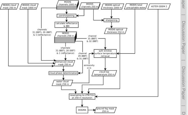
All other inputs (cf. Fig. 6) are based on MODIS Collection 051 Level 1B and Level

10

2 products. MODIS data has been chosen instead of the data of geostationary satel-lites (e.g. the Japanese Himawari series covering the area of Taiwan) because of the combination the long time span for which the data is available (MODIS: since 1999 (Terra)/2002 (Aqua); Himawari 7: since 2006; Himawari 8: since 2015) and its rela-tively high spatial resolution (MODIS: up to 250 m; Himawari 7: up to 1000 m; Himawari

15

8: up to 500 m). The latter is necessary due to the complex topography of Taiwan’s mountains.

The cloud optical thickness is based on the MODIS MOD06 optical thickness derived from radiative transfer calculations (Platnick et al., 2015). As it is only available for daytime scenes, the application of DOGMA is restricted to those. (cf. Sect. 3.2)

20

Since fog is (with the exception of ice fog that can only be found in polar latitudes, Oke, 1978) completely in the water phase, DOGMA is only applied on water clouds. Additionally to the inputs mentioned in Sect. 2.2 a cloud mask including information about the cloud phase thus is necessary as an input. It is based on the MODIS MOD35 cloud mask product (cf. Sect. 3.3).

25

(9)

AMTD

8, 12155–12201, 2015

areas

H. M. Schulz et al.

Title Page

Tables Figures

◭ ◮

Back Close

Full Screen / Esc

Discussion

P

a

per

|

Discussion

P

a

per

|

Discussion

P

a

per

|

Discussion

P

a

per

|

are calculated for all water cloud pixels from MODIS thermal infrared (TIR) window channels (cf. Sect. 3.4).

To make use of the full 250 m resolution of MODIS, which is only available in the visible bands 1 and 2, different techniques (cf. Sects. 3.1–3.4) are applied to sharpen those inputs using the MODIS high-resolution bands.

5

3.1 Pan-sharpening of MODIS channels

MODIS channels are not necessary as an input for DOGMA. Some are, however, re-quired to sharpen other MODIS products needed as an input. Therefore several in-frared channels are transferred to the 250 m resolution of MODIS channels 1 and 2 using a suited pan-sharpening technique by Schulz et al. (2012). According to this

10

method a high-resolution satellite channel is degraded to match the resolution of the low-resolution channel that is to be sharpened. This is done by averaging each group of 4×4 high-resolution pixels the area of which corresponds to one and the same low-resolution pixel. Then a potential regression is used to explain the pixel values of the low-resolution channel with the pixel values of the degraded high-resolution channel.

15

The same regression is applied on the original high-resolution channel in order to ob-tain a high-resolution version of the low-resolution channel. This procedure is, however, not applied on a scene globally as that would lead to a low coe_fficient of determination of the regression. This would result in a bad quality of the sharpened image. Instead, a channel is sharpened pixelwise using a different regression for each pixel. Each

re-20

gression is based on an approximately round moving window with a diameter of 5 pixels centred at the pixel that is to be sharpened.

For DOGMA data pre-processing the pan-sharpening technique has been adapted to MODIS data. Since MODIS has two channels in the resolution of 250 m, both of them were degraded and used to sharpen the low-resolution channels using a multiple

25

(10)

AMTD

8, 12155–12201, 2015

areas

H. M. Schulz et al.

Title Page

Tables Figures

◭ ◮

Back Close

Full Screen / Esc

Discussion

P

a

per

|

Discussion

P

a

per

|

Discussion

P

a

per

|

Discussion

P

a

per

|

process of 4×4 high-resolution pixels each high-resolution pixel is weighted by the sensor’s spatial response function (taken from Huang et al., 2002) of the low-resolution pixel that is to be sharpened.

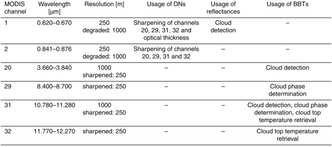
The described method is used to sharpen the unitless digital number (DN) values of the MODIS channels 20, 29, 31 and 32 as distributed via the MODIS MOD02/MYD02

5

product. After sharpening, the DNs of these channels are transferred to radiances using scale and offset values included in the MOD02/MYD02 product. The inverse Planck Function is used to calculate Black Body Temperature (BBT) values from the radiances. BBTs are also calculated from the 1000 m DNs of the channels 20 and 31. From the DNs of channel 1 the reflectance is calculated using the appropriate scale and

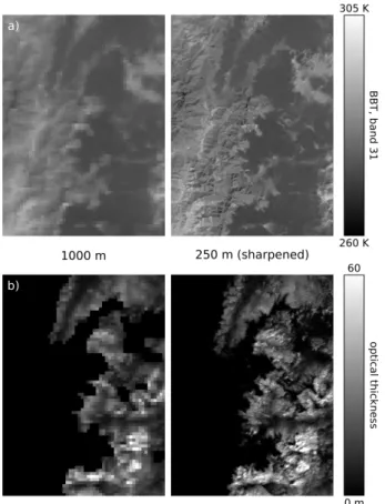
10

o_ffset values from the MOD02/MYD02 product. A sharpening result for channel 31 is exemplarily shown in Fig. 7. An overview of the used channels is given in Table 3.

3.2 Cloud optical thickness

Over land surfaces the MOD06 optical thickness is mostly based on channel 1 (Platnick et al., 2003). Therefore an slightly adapted version of the pan-sharpening method used

15

to process the 1000 m MODIS imagery (cf. Sect. 3.1) is suited to sharpen it. Instead of a multiple regression a simple regression incorporating only channel 1 (instead of channel 1 and 2) as the independent variable is used. An example result is shown in Fig. 7.

3.3 Cloud mask

20

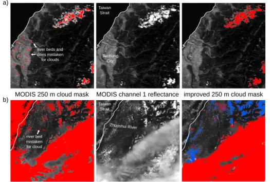
As it is based on the solar MODIS high resolution channels 1 and 2 only, the 250 m cloud mask included in the MOD35 cloud mask product does not contain information about the cloud phase. Furthermore it is, for some scenes, heavily flawed in the area of Taiwan. Cities and riverbeds with high reflectance values are often wrongly classified as clouds (cf. Fig. 8). These problems do not occur in the MOD35 1000 m cloud masks.

25

(11)

AMTD

8, 12155–12201, 2015

areas

H. M. Schulz et al.

Title Page

Tables Figures

◭ ◮

Back Close

Full Screen / Esc

Discussion

P

a

per

|

Discussion

P

a

per

|

Discussion

P

a

per

|

Discussion

P

a

per

|

1000 m cloud mask as a reference and sharpened as well as not-sharpened MODIS imagery as its basis. Before any further processing is applied thin cirrus are removed from the 1000 m MOD35 cloud mask based on the included cloud classification.

Cermak and Bendix (2008) have shown that a threshold applied on the difference BBTTIR−BBTMIR(further referred to as diff250and diff1000for the 250 m and the 1000 m

5

version) between BBT values in the thermal (TIR) and medium infrared (MIR) is well suited to distinguish between cloud-contaminated and clear pixels using a threshold. The difference values are clearly negative for cloudy pixels and near to 0 for clear surfaces. For MODIS this difference can be calculated from the channels 31 (TIR) and 20 (MIR).

10

To identify a suitable threshold for a certain scene several iteratively adapted thresh-olds are applied on diff1000 in order to obtain masks in the 1000 m resolution. Those

masks are compared to the MOD35 1000 m cloud mask in terms of the percentage of pixels being classified in agreement between the cloud mask derived from di_ff₁₀₀₀and the MODIS reference product. The threshold resulting in the best agreement is chosen.

15

Since clouds are highly reflective in the visible spectrum, a threshold can also be applied on the reflectance of channel 1 (further referred to as ref₂₅₀and ref₁₀₀₀for the 250 m and the 1000 m version) to distinguish between cloud-covered and cloud-free pixel to some degree. This threshold is determined in the same iterative way as the threshold derived from di_ff₁₀₀₀.

20

These two thresholds can then be applied on diff250 and ref250. The results are two

cloud masks in 250 m that still contain several flaws (e.g. cities and river beds being classified as clouds due to their high albedo in the channels 1 and 20). As the flaws often are in different areas the two cloud masks can be combined to a new cloud mask (further referred to as global cloud mask) that consists only of the pixels classified as

25

(12)

AMTD

8, 12155–12201, 2015

areas

H. M. Schulz et al.

Title Page

Tables Figures

◭ ◮

Back Close

Full Screen / Esc

Discussion

P

a

per

|

Discussion

P

a

per

|

Discussion

P

a

per

|

Discussion

P

a

per

|

and ref₂₅₀ covered by p are then classified as cloud-contaminated or cloud-free using these thresholds. The results from the local approach and the global cloud mask are combined to a final 250 m cloud mask. A pixel is considered as cloudy if clouds are present according to the global cloud mask and

(a) the pixel is cloud-contaminated according to the local thresholds applied on diff250

5

and ref250or

(b) the pixel is unambiguously cloudy according to the value of diff250(diff250is below

the diff250 value of at least 50 % of the pixels in the 20 pixels×20 pixels window

that are considered as clouds according the MODIS 1000 m cloud mask).

The resulting mask does still not differentiate between water, ice and mixed phase

10

clouds. Mixed and ice phase clouds are detected using the same threshold approach that is incorporated in the MODIS cloud phase classification. It is mainly based on ra-diative transfer calculations that have shown that the difference BBT29−BBT31between

the MODIS channels 29 and 31 is high for ice clouds and low for water clouds (Chylek et al., 2006). Also BBTs from channel 31 can be incorporated to detect clouds that are

15

obviously too cold to be in the water phase. The MODIS cloud classification combines these two approaches to identify cloud pixels that are not or not solely in the liquid phase as follows (Platnick et al., 2003):

(a) mixed phase: 238<BBT31<268 K and−0.25≤BBT29−BBT31<0.5 K

(b) ice phase: BBT₃₁≤238 K or BBT₂₉−BBT₃₁≥0.5 K

20

Examples for the enhanced 250 m cloud mask are shown in Fig. 8.

3.4 Cloud top temperature

Cloud top temperatures are calculated for all water cloud pixels from the sharpened BBTs of the MODIS TIR window channels 31 and 32 using a split-window algorithm proposed by Jiménez-Munõz and Sobrino (2008). It allows to correct for atmospheric

(13)

AMTD

8, 12155–12201, 2015

areas

H. M. Schulz et al.

Title Page

Tables Figures

◭ ◮

Back Close

Full Screen / Esc

Discussion

P

a

per

|

Discussion

P

a

per

|

Discussion

P

a

per

|

Discussion

P

a

per

|

absorption as well as emissivity effects. The latter, however, are ignored in our cloud top temperature retrieval as an emissivity of 1 for the cloud surface is assumed. This approximation for water clouds is possible for TIR wavelengths, if the cloud is supposed to have a thickness of at least several tens of meters (cf. e.g. Yamamoto et al., 1970; Hunt, 1973). The total atmospheric water vapour content, which is needed as an

ad-5

ditional input for the cloud top temperature retrieval, is taken from the MOD05/MYD05 total precipitable water product. It is resampled to the 250 m resolution without sharp-ening.

4 Methodology

4.1 DOGMA – detailed description

10

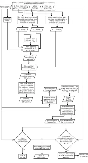
DOGMA is fed with the inputs described in Sect. 3 (cf. Fig. 9). Pixels classified as ice cloud or mixed phase cloud in the 250 m cloud mask are removed from the analysis and marked as unclassifiable as they might block the view to lower fog layers. The algorithm runs through each 250 m water cloud pixel p of a MODIS scene and calculatesρ_{below p},

ρ_{above p}andρ_di_ff_p(cf. Fig. 10a) from a round window with a diameter of 40 pixels around

15

p as described in Sect. 2.2. The scene is then scanned for local maxima of ρ_di_ff_p. in order to detect pixels at the cloud base height (further referred to as CBH pixels). This is done by comparing each water cloud pixel p to all other water cloud pixels in a round window with a diameter of 20 pixels centred at p. Pixels which are higher than the lowest direct neighbour of p or lower than the highest direct neighbour of p

20

are excluded from this comparison as they would (if p is actually a CBH pixel) most probably be CBH pixels of the same cloud base as p. p is marked as alow certainty CBH pixel(cf. Fig. 10b) if

(a) p has a higherρ_di_ff_pthan all the pixels it is compared to and (b) ρ_di_ff_pis below 0 and

(14)

AMTD

8, 12155–12201, 2015

areas

H. M. Schulz et al.

Title Page

Tables Figures

◭ ◮

Back Close

Full Screen / Esc

Discussion

P

a

per

|

Discussion

P

a

per

|

Discussion

P

a

per

|

Discussion

P

a

per

|

(c) ρ_{above p}is clearly negative (an empirically derived threshold of−0.3 is used) and (d) p has according to the DEM a slope elevation of at least 7.2 % (This is checked as

the considerations in Sect. 2.2 are all based on the assumption of mountainous terrain).

Asρ_di_ff_p and ρ_{above p} are calculated from relatively small windows, small scale

vari-5

ations of the cloud bottom height can be captured well. On such a local level random small-scale gradients of the cloud thickness or the extinction coefficient that spatially coincide with an increase or decrease in terrain height could be mistaken for correla-tions that are caused by a cloud being cut offby the terrain. For bigger windows, result-ing in a bigger sample size of the correlations, such small-scale gradients have a much

10

lower impact. Thereforeρ_{above p} is calculated again (further referred to asρ_{above p, 120}) for each low certainty CBH pixel p. This is done based on the optical thickness and height of all pixels in a round window with a diameter of 120 pixels centred around p. For a window of this size the assumption of a negligible variability of cloud top height, cloud bottom height and coefficient of extinction inside the window may not be fulfilled. If

15

p is actually a CBH pixel, the 120 pixels window could, for example contain water cloud pixels with a higher elevation than p that are free of ground fog due to variations of the cloud base height. Therefore the correlation may not reach very low values even for CBH pixel. Thus, a relatively high threshold of 0 is applied onρ_{above p, 120}. Ifρ_{above p, 120}

is below that value, p can be regarded as a CBH pixel withmedium certainty.

20

As real CBH pixels should be a part of a cloud base that is formed by several CBH pixels, CBH pixels that are surrounded by other CBH pixels should have an increased probability of being real CBH pixels. Therefore for each medium certainty CBH pixel p, it is checked if at least 10 other medium certainty CBH pixel can be found in a round window with a diameter of 40 pixels centred at p. If that is the case, p is marked as

25

ahigh certainty CBH pixel.

(15)

de-AMTD

8, 12155–12201, 2015

areas

H. M. Schulz et al.

Title Page

Tables Figures

◭ ◮

Back Close

Full Screen / Esc

Discussion

P

a

per

|

Discussion

P

a

per

|

Discussion

P

a

per

|

Discussion

P

a

per

|

tected CBH pixels (which is necessary to capture small scale variations in the cloud bottom height as precise as possible), DOGMA goes back to the original low certainty CBH pixels and filters them again based on their vertical distance to an assumed cloud base surface that can be defined from the high certainty CBH pixels. This cloud base surface is modelled for each water cloud entity separately by interpolating the heights

5

of all high certainty CBH pixel belonging to that cloud entity using Inverse Distance Weighting (IDW, Shepard, 1968). All low certainty CBH pixels that are within a vertical distance of less than 400 m to this surface (further referred to asfinal CBH pixels) are used for the discrimination of ground fog.

For the final ground fog discrimination, the heights of all final CBH pixels of each

10

water cloud entity as well as their temperature taken from the cloud top temperature image are interpolated using IDW interpolation (cf. Fig. 10c). Each pixel p in which the interpolated height of the cloud base is below or equal to the height taken from the DEM are ground fog pixels if the IDW interpolated temperature of p is not more than 3 K higher than the temperature taken from the cloud top temperature image. If

15

the measured temperature was much colder, p would be significantly higher than the pixels used for the IDW interpolation. Therefore it would either belong to another cloud level or the assumption of a cloud top surface that can locally be approximated as plane would be wrong for p.

So far the existence of a cloud base surface that has a one-dimensional intersection

20

with the terrain has been assumed. If a fog cloud does, however, touch the terrain with its entire base (=complete valley fill), such an intersection does not exist. Therefore the cloud would not be identified as fog by the tests described so far. In order to detect those clouds nevertheless, each cloud entity from the water cloud mask is further ex-amined if no fog has been detected in it. For each pixel p of the entityρ is calculated

25

from the pixels in a round window with a diameter of 40 pixels that is centred at p. If the median of allρis below−0.3, all pixels of the entity are considered as ground fog pixels.

(16)

AMTD

8, 12155–12201, 2015

areas

H. M. Schulz et al.

Title Page

Tables Figures

◭ ◮

Back Close

Full Screen / Esc

Discussion

P

a

per

|

Discussion

P

a

per

|

Discussion

P

a

per

|

Discussion

P

a

per

|

4.2 Methodology of validation

For many areas METeorological Aerodrome Reports (METARs) are ideally suited to validate ground fog detection schemes (cf. e.g. Cermak and Bendix, 2011; Schulz et al., 2012). These reports are based on weather observations from airports and in-clude cloud base heights as well as information about the visibility at ground level. In

5

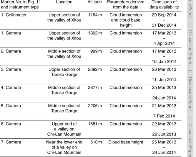
Taiwan, however, all airports are located in the plains in the outer parts of the island and not in the mountainous area where DOGMA can be applied (dark red area Fig. 10b). Considering this lack of data, several cameras of the type PlotWatcher Pro (Day 6 Out-doors, LLC, USA) were installed in the mountainous parts of the island. The cameras are set up to take a photo each minute and save it to a SD card. Additionally, the data

10

of a CL31 ceilometer (Vaisala, Finland) installed in Xitou has been used (cf. Fig. 11; Table 4).

Table 4 gives an overview about the time spans in which the different instruments have captured data. For those time spans DOGMA ground fog products were gener-ated from the data of all Terra and Aqua daytime overflights over Taiwan. The DOGMA

15

ground fog product (cf. Sect. 4.2.1) as well as the IDW interpolated cloud base surface (cf. Sect. 4.2.2) have been compared to the camera and ceilometer data in order to assess their quality.

4.2.1 Validation of the ground fog product

The cameras 1 to 6 are located at positions that are often cloud immersed. All of

20

their images taken at the time of MODIS overflights were manually classified into the categories “fog free” or “fog immersed”. Also from the ceilometer data captured at over-flight times, information about the cloud immersion of the instrument were extracted. Each camera and ceilometer reference observation was then compared to the DOGMA ground fog product pixel that is correspondent in space and time. Ice cloud and mixed

25

(17)

ta-AMTD

8, 12155–12201, 2015

areas

H. M. Schulz et al.

Title Page

Tables Figures

◭ ◮

Back Close

Full Screen / Esc

Discussion

P

a

per

|

Discussion

P

a

per

|

Discussion

P

a

per

|

Discussion

P

a

per

|

ble the following statistical measures have been calculated (cf. Mason (2003); Matthew (1975); see Appendix A for formulas):

– Proportion Correct (PC);

– Bias;

– Probability Of Detection (POD);

5

– Probability Of False Detection (POFD);

– False Alarm Rate (FAR);

– Matthews Correlation Coefficient (MCC).

4.2.2 Validation of the DOGMA cloud base height

As the quality of the DOGMA ground fog product is a direct result of the cloud base

10

surface height (cf. Fig. 10c), the latter has been validated separately. This was done using the ceilometer as well as camera 7. The ceilometer is located in the valley of Xitou where a high fog frequency can be observed. The camera is located near the lower end of a valley on Chi-Lang Mountain facing up the valley. While the camera location is usually fog free, the upper parts of the valley are often fog immersed. The

15

intersection between the cloud base and the terrain can be observed by the camera in these cases.

Cloud base validation using ceilometer data

The ceilometer validation has been conducted for all MODIS overflights in which the DOGMA cloud base product provides information for the ceilometer location and the

20

(18)

AMTD

8, 12155–12201, 2015

areas

H. M. Schulz et al.

Title Page

Tables Figures

◭ ◮

Back Close

Full Screen / Esc

Discussion

P

a

per

|

Discussion

P

a

per

|

Discussion

P

a

per

|

Discussion

P

a

per

|

has been calculated between ceilometer reference data and the extracted cloud base heights. All scenes in which the ceilometer obtained cloud base height is above the height of the highest pixel in the valley of Xitou that is cloud covered (according to the 250 m water cloud mask) were excluded from this calculation. This was necessary as DOGMA extracts the height of the cloud base from the DEM and is therefore – as

5

a matter of principle – not able to detect any cloud base that does not touch the terrain. For ground fog detection information about higher cloud bases is not of interest. Also scenes in which the DOGMA cloud base is below the ceilometer location needed to be excluded from the calculation as ceilometer data (which is only available if the cloud base is above the ceilometer) would only be available if the DOGMA cloud base height

10

is wrong. This would result in a biased validation.

Cloud base validation using camera data

While cloud bottom heights recorded by the ceilometer could be directly compared to the height of the DOGMA cloud base, the camera footage needed to be processed manually in order to obtain reference cloud bottom heights. All images taken at MODIS

15

overflights were assessed to determine whether the captured slopes of Chi-Lan Moun-tain are cloud immersed as it is shown in Fig. 12. Scenes for which that is not the case and scenes for which the weather conditions (e.g. ground fog at the camera location) did not allow an unequivocal identification of the cloud base where excluded from fur-ther analysis. For the remaining scenes the intersection of the cloud base height and

20

the terrain was marked manually in the image (red lines in Fig. 12). For those image pixels that have been marked as intersection pixels the altitude was extracted from the ASTER GDEM 2 reprojected to the view of the camera (cf. Schulz et al. (2014) for details about the reprojection). IDW interpolation has been used to model a cloud base surface from the heights and positions of those pixels in a resolution of 250 m for

25

(19)

AMTD

8, 12155–12201, 2015

areas

H. M. Schulz et al.

Title Page

Tables Figures

◭ ◮

Back Close

Full Screen / Esc

Discussion

P

a

per

|

Discussion

P

a

per

|

Discussion

P

a

per

|

Discussion

P

a

per

|

deviations in height between all pixels of the camera obtained cloud base surface and the corresponding DOGMA cloud base surface pixels was then calculated. The result is a single value for each scene that describes the deviation between the camera ob-tained cloud base and the DOGMA cloud base for the whole view shed of the camera. From those deviations the mean deviation has been calculated.

5

5 Validation results and discussion

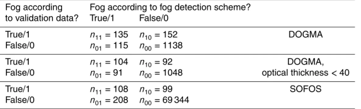
The results of the validation of the DOGMA ground fog product are shown in Tables 5 and 6. Also the results of a validation carried out by Cermak and Bendix (2011) for their own method using METAR data from a European domain are included. As the two validations are based on different data sets from different areas, they should not

10

be directly compared to each other. The validation by Cermak and Bendix should only be seen as a reference for the current quality of ground fog detection from space born sensors.

As shown in Table 6 both methods have a relatively similar overall fog detection quality (MCC). DOGMA tends to underestimate the fog frequency while the method by

15

Cermak and Bendix generally overestimates it (Bias). In detail that means that a lower ratio of fog pixels is correctly classified as fog by DOGMA than by the method of Cer-mak and Bendix (POD) but also that a lower ratio of all pixels that are classified as fog contaminated is wrongly classified (FAR). A higher ratio of fog free pixels is, however, wrongly classified as fog by DOGMA (POFD). The main issue with both methods is

20

a relatively high FAR in combination with a relatively low POD.

The shortcomings of DOGMA might mostly be caused by clouds that can not locally be approximated as plane-parallel and horizontally homogeneous as it is assumed by the method. Also clouds with a very high optical thickness that do often cover Taiwan can cause problems. The footage of the cameras shows that optically thick clouds do

25

(20)

AMTD

8, 12155–12201, 2015

areas

H. M. Schulz et al.

Title Page

Tables Figures

◭ ◮

Back Close

Full Screen / Esc

Discussion

P

a

per

|

Discussion

P

a

per

|

Discussion

P

a

per

|

Discussion

P

a

per

|

situation. An optical thickness of 40 – a value that is surpassed in 13.31 % of the pixels that have been used for the validation – corresponds to a transmittance of 4.24×1018. With such a low transmittance almost no light – and therefore hardly any information – from the cloud base does reach the sensor. In order to assess the impact of those very thick clouds, a validation excluding all reference observations during which the camera

5

or ceilometer has been located below a cloud with an optical thickness of more than 40 has been carried out. As shown in Table 6 this increases the overall detection quality (MCC), mainly due to a better POD.

The mean deviation of the DOGMA cloud base height is given in Table 7. DOGMA does not directly calculate a cloud base height. Instead CBH pixels are detected in

10

a two-dimensional image (cf. Sect. 4.1). As the validated DOGMA cloud base height is interpolated from the height of the DEM extracted from these pixels, its precision is (if inaccuracies of the interpolation are ignored) a result of the correctness of the de-tection of CBH pixels in combination with the topography and its mapping in the 250 m resolution of the DEM. The mean steepness of the slopes of both valleys incorporated

15

in the cloud base validation is approximately 50–60 %. As a pixel with sides of 250 m in length has a diagonal of about 354 m, height di_fferences of 177 m (50 % of 354 m) to 212.4 m (60 % of 354 m) inside a single pixel are possible and height differences be-tween 125 m (50 % of 250 m) an 150 m (60 % of 250 m) are unavoidable. This means that even CBH pixels that have been detected in the correct position may result in

rela-20

tively imprecise cloud base heights, although the delimitation of the fog immersed area would be perfect. Conversely, this implies that the∼200 m error of the DOGMA cloud base is the result of a relatively small mean error of less than two pixels in the hori-zontal positions of the CBH pixels. Therefore the DOGMA cloud base height product is suited for ground fog delimitation but should not be used for other purposes.

(21)

AMTD

8, 12155–12201, 2015

areas

H. M. Schulz et al.

Title Page

Tables Figures

◭ ◮

Back Close

Full Screen / Esc

Discussion

P

a

per

|

Discussion

P

a

per

|

Discussion

P

a

per

|

Discussion

P

a

per

|

6 Conclusion and outlook

Common fog detection schemes that have been developed for radiation fog are not applicable in Taiwan as they rely on assumptions (cf. Sect. 2.1) that are not met by most fog occurrences in Taiwan. Therefore the presented method has been devel-oped. DOGMA does not calculate the cloud base height from the difference between

5

the cloud top height and the cloud thickness. Instead pixels at the cloud base are di-rectly detected using a statistical approach that is based on a negative Spearman’s rank correlation coefficient between the optical thickness and the terrain height of fog immersed pixels extracted from the DEM. As it relies on clouds that can be at least locally approximated as plane-parallel and horizontally homogeneous and also the

10

MOD 06 optical thickness product is based on a radiative transfer calculations using a plane-parallel cloud model (Platnick et al., 2003), also DOGMA does rely on some assumptions. The necessary degree of plane-parallelism and horizontal homogeneity is, however, low enough, so that the method is applicable to sea of clouds situations (cf. Fig. 2) as they are typical for Taiwan. As the comparison to the method of Cermak and

15

Bendix (cf. Sect. 5) has shown, the overall quality of DOGMA’s fog detection is (despite some problems with fog clouds with a very high optical thickness) comparable to that of a modern fog detection scheme developed and validated for the temperate zones. It therefore seems to be applicable for the creation of ground fog frequency maps that can be used for the country-wide mapping of Taiwan’s cloud forests.

20

DOGMA is restricted to mountainous areas. If perfectly plane-parallel and horizon-tally homogeneous fog clouds are assumed, it should work even for slightest slopes. As those perfect conditions actually won’t be met, it will be the subject of future work to find out for which areas DOGMA is suited. It would e.g. be conceivable that the method works for very plain radiation fog in the valleys of low mountain ranges.

25

(22)

AMTD

8, 12155–12201, 2015

areas

H. M. Schulz et al.

Title Page

Tables Figures

◭ ◮

Back Close

Full Screen / Esc

Discussion

P

a

per

|

Discussion

P

a

per

|

Discussion

P

a

per

|

Discussion

P

a

per

|

implementation of DOGMA due to its high spatial resolution and the long time span for which its data is available. The drawback of a polar-orbiting satellite is, however, its bad temporal coverage. Therefore the imagery of the new Himawari 8 satellite with a res-olution of up to 500 m pixel−1 and a sampling rate of 10 min would be well suited for future implementations of DOGMA in order to obtain information about ground fog in

5

Taiwan.

Appendix A: Formulas used in the validation of the ground fog product

The following formulas were used for the calculation of the statistical measure used in Sect. 4.2.1. Cf. Table 5 for explanations ofn₁₁,n₁₀,n₀₁ andn₀₀.

MCC=_p n11·n00−n01·n10

(n₁₁₊n₀₁)·(n₁₁₊n₁₀)·(n₀₀₊n₀₁)·(n₀₀₊n₁₀)

(A1)

10

PC=_n n11+n00

11+n10+n01+n00

(A2)

Bias=n_n11+n01

11+n10

(A3)

POD₌ n11

n₁₁₊n₀₀ (A4)

POFD= n01

n₀₁₊n₀₀ (A5)

FAR= n01

n₁₁₊n₀₁ (A6)

15

(23)

AMTD

8, 12155–12201, 2015

areas

H. M. Schulz et al.

Title Page

Tables Figures

◭ ◮

Back Close

Full Screen / Esc

Discussion

P

a

per

|

Discussion

P

a

per

|

Discussion

P

a

per

|

Discussion

P

a

per

|

References

Bendix, J. and Bachmann, M.: Climatology of fog layers in the Alpine region – a study based on AVHRR data, in: Proceedings of the 6th AVHRR Data Users’ Meeting, Belgirate, Italy, 29 June–2 July 1993, 237–248, 1993.

Bendix, J., Thies, B., Cermak, J., and Nauß, T.: Ground fog detection from space based on

5

MODIS daytime data – a feasibility study, Weather Forecast., 20, 989–1005, 2005.

Bruijnzeel, L. A., Mulligan, M., and Scatena, F. N.: Hydrometeorology of tropical montane cloud forests: emerging patterns, Hydrol. Process., 25, 465–498, 2010.

Cermak, J. and Bendix, J.: A novel approach to fog/low stratus detection using Meteosat 8 data, Atmos. Res., 87, 279–292, 2008.

10

Cermak, J. and Bendix, J.: Detecting ground fog from space – a microphysics-based approach, Int. J. Remote Sens., 12, 3345–3371, 2011.

Chang, F.-L. and Li, Z.: Estimating the vertical variation of cloud droplet effective radius using multispectral near-infrared satellite measurements, J. Geophys. Res., 107, 7-1–7-12, 2002. Chu, H.-S., Chang, S.-H., Klemm, O., Lai, C.-W., Lin, Y.-Z, Wu, C.-C., Lin, J.-Y., Jiang, J.-Y.,

15

Chen, J., Gottgens, J. F., and Hsia, Y.-J.: Does canopy wetness matter? Evapotranspiration from a subtropical montane cloud forest in Taiwan, Hydrol. Process., 28, 1190–1214, 2012. Chylek, P., Robinson, S., Dubey, M. K., King, M. D., Fu, Q., and Clodius, W. B.: Comparison

of near-infrared and thermal infrared cloud phase detections, J. Geophys. Res.-Atmos., 111, D20203, 1–8, 2006.

20

Hijmans, R. J., Cameron, S. E., Parra, P. G., and Jarvis, A.: Very high resolution interpolated climate surfaces for global land areas, Int. J. Climatol., 25, 1965–1978, 2005.

Hsieh, C. F.: Composition, endemism and phytogeographical affinities of the Taiwan flora, Tai-wania, 47, 298–310, 2002.

Huang, C., Townshend, J. R. G., Liang, S., Kalluri, S. N. V, and DeFries, R. S.: Impact of

sen-25

sor’s point spread function on land cover characterization: assessment and deconvolution, Remote Sens. Environ., 80, 203–212, 2002.

Hunt, G. W.: Radiative properties of terrestrial clouds at visible and infra-red wavelengths, Q. J. Roy. Meteor. Soc., 99, 346–369, 1973.

Hutchison, K. D.: The retrieval of cloud base heights from MODIS and three-dimensional cloud

30

(24)

AMTD

8, 12155–12201, 2015

areas

H. M. Schulz et al.

Title Page

Tables Figures

◭ ◮

Back Close

Full Screen / Esc

Discussion

P

a

per

|

Discussion

P

a

per

|

Discussion

P

a

per

|

Discussion

P

a

per

|

Jiménez-Munõz, J.-C. and Sobrino, J. A.: Split-window coefficients for land surface temperature retrieval from low-resolution thermal infrared sensors, IEEE Geosci. Remote S., 5, 806–809, 2008.

Li, C.-F., Chytr´y, M., Zelen´y, D., Chen, M.-Y., Chen, T.-Y., Chiou, C.-R., Hsia, Y.-J., Liu, H.-Y., Yang, S.-Z., Yeh, C.-L., Wang, J.-C., Yu, C.-F., Lai, Y.-J., Chao, W.-C., and Hsieh, C.-F.:

5

Classification of taiwan forest vegetation, Appl. Veg. Sci., 4, 698–719, 2013.

Li, C. F., Zelen´y, D., Chytr´y, M., Chen, M.-Y., Chen, T.-Y., Chiou, C.-R., Hsia, Y.-J., Liu, H.-Y., Yang, S.-Z., Yeh, C.-L., Wang, J.-C., Yu, C.-F., Lai, Y.-J., Guo, K., and Hsieh, C.-F.: Chamae-cyparis montane cloud forest in Taiwan: ecology and vegetation classification, Ecol. Res., 5, 771–791, 2015.

10

Mason, I. B.: Binary events, in: Forecast Verification – a Practitioner’s Guide in Atmospheric Science, edited by: Jolliffe, I. T. and Stephenson, D. B., John Wiley & Sons, Chicester, UK, 37–76, 2003.

Matthews, B. W.: Comparison of the predicted and observed secondary structure of T4 phage lysozyme, Biochim. Biophys. Acta, 405, 442–451, 1975.

15

Menzel, W. P., Smith, W. L., and Stewart, T. R.: Improved cloud motion wind vector and altitude assignment using VAS, J. Clim. Appl. Meteorol., 3, 377–384, 1983.

Mildenberger, K., Beiderwieden, E., Hsia, Y.-J., and Klemm, O.: CO₂ and water vapor fluxes above a subtropical mountain cloud forest – the effect of light conditions and fog, Agr. Forest Meteorol., 149, 1730–1736, 2009.

20

Minnis, P., Kratz, D. P., Coakley, J. A., King, M. D., Garber, D. P., Heck, P. W., Mayor, S., Young, D. F., and Arduini, R. F.: Cloud optical property retrieval (subsystem 4.3), in: Clouds and the Earth’s Radiant Energy System (CERES) Algorithm Theoretical Basis Document, edited by: Wielicki, B. A., Barkstrom, B. R., Baum, B. A., Blackmon, M., Cess, R. D., Char-lock, T. P., Coakley, J. A., Crommelynck, D. A., Green, R. N., Kandel, R., King, M. D.,

25

Lee, R. B., Miller, A. J., Minnis, P., Ramanathan, V., Randall, D. R., Smith, G. L., Stowe, L. L., and Welch, R. M., National Aeronautics and Space Administration Langley Research Center, Hampton, VA, USA, 135–176, 1997.

Mulligan, M. and Burke, S. M.: DFID FRP Project ZF0216 Global Cloud Forests and Environ-mental Change in a Hydrological Context, Final Report, DFID, London, UK, 2006.

30

(25)

AMTD

8, 12155–12201, 2015

areas

H. M. Schulz et al.

Title Page

Tables Figures

◭ ◮

Back Close

Full Screen / Esc

Discussion

P

a

per

|

Discussion

P

a

per

|

Discussion

P

a

per

|

Discussion

P

a

per

|

Platnick, S., King, M. D., Ackermann, S. A., Menzel, W. P., Baum, B. A., Riedi, J. C., and Frey, R. A.: The MODIS cloud products: algorithms and examples from Terra, IEEE T. Geosci. Remote, 2, 459–473, 2003.

Postel, S. L. and Thompson Jr., B. H.: Watershed protection: capturing the benefits of nature’s water supply services, Nat. Resour. Forum, 29, 98–108, 2005.

5

Schulz, H. M., Thies, B., Cermak, J., and Bendix, J.: 1 km fog and low stratus detection using pan-sharpened MSG SEVIRI data, Atmos. Meas. Tech., 5, 2469–2480, doi:10.5194/amt-5-2469-2012, 2012.

Schulz, H. M., Chang, S.-C., Thies, B., and Bendix, J.: Automatic cloud top height determination in mountainous areas using a cost-effective time-lapse camera system, Atmos. Meas. Tech.,

10

7, 4185–4201, doi:10.5194/amt-7-4185-2014, 2014.

Shepard, D.: A two-dimensional interpolation function for irregularly-spaced data, in: Proceed-ings of the 23rd ACM National Conference, Princeton, USA, 27–29 August 1968, 517–524, 1968.

Thies, B., Groos, A., Schulz, M., Li, C.-F., Chang, S.-C., and Bendix, J.: Frequency of low clouds

15

in Taiwan retrieved from MODIS data and its relation to cloud forest occurrence, Rem. Sens., 7, 12986–13004, 2015.

United States Geological Survey: Global data explorer, available at: http://gdex.cr.usgs.gov/ gdex/ (last access: 18 November 2015), 2013.

Yamamoto, G., Tanaka, M., and Asano, S.: Radiative transfer in water clouds in the infrared

20

region, J. Atmos. Sci., 27, 282–292, 1970.

Yi, L., Zhang, S.-P., Thies, B., Shi, X.-M., Trachte, K., and Bendix, J.: Spatio-temporal detection of fog and low stratus top heights over the Yellow Sea with geostationary satellite data as a precondition for ground fog detection – a feasibility study, Atmos. Res., 151, 212–223, 2015.

(26)

AMTD

8, 12155–12201, 2015

areas

H. M. Schulz et al.

Title Page Abstract Introduction Conclusions References Tables Figures ◭ ◮ ◭ ◮ Back Close

Full Screen / Esc

Printer-friendly Version Interactive Discussion Discussion P a per | Discussion P a per | Discussion P a per | Discussion P a per |

Table 1.Different cloud height retrieval methods.

Reference Basic idea of the method Problems

Menzel et al. (1983)

CO₂ slicing: due to CO₂ absorp-tion increasing with wavelength in the CO₂ band around 15 µm, diff er-ent channels in this band are sen-sitive to different levels in the atmo-sphere.

The CO₂ absorption is very high for low levels (<3 km) of the atmo-sphere. This results in bad signal-to-noise ratios for low level clouds such as fog.

Bendix and Bachmann (1993)

DEM extraction: for a fog entity that is horizontally restricted by the ter-rain the height of its outermost pix-els can be read from a DEM.

Only possible for fog that is re-stricted by the terrain in its horizon-tal extent.

Yi et al. (2015) The top height of radiation fog that is restricted in its vertical extent by an temperature inversion is equal to the base height of that inversion. The base height of the inversion can be calculated from satellite data.

Highly experimental.

Works only for radiation fog. The fog occurrence in Taiwan, however, is mainly caused by moist air masses being uplifted by the Taiwanese mountains (Li et al., 2015).

e.g. Cermak and Bendix (2008); Platnick et al. (2003)

Under the assumption of a fixed negative temperature lapse rate or an atmospheric profile the cloud top height can be calculated from the cloud top temperature.

(27)

AMTD

8, 12155–12201, 2015

areas

H. M. Schulz et al.

Title Page Abstract Introduction Conclusions References Tables Figures ◭ ◮ ◭ ◮ Back Close

Full Screen / Esc

Printer-friendly Version Interactive Discussion Discussion P a per | Discussion P a per | Discussion P a per | Discussion P a per |

Table 2.Different cloud thickness retrieval methods.

Authors Basic idea of the method Problems

Hutchinson (2002)

As the liquid water path (LWP) is the column inte-gration of the the liquid water content (LWC), the cloud thickness can be calculated from the satel-lite retrieved liquid water path (LWP) under the assumption of a fixed liquid water content (LWC) for certain cloud types.

The LWC is vertically not constant. For thin clouds, however, a verti-cally constant LWC can be approxi-mated.

Minnis et al. (1997)

The cloud thickness is calculated from the satel-lite retrieved cloud optical thickness using empir-ical formulas. For clouds in different heights, dif-ferent formulas are used.

Due to oversimplification, the ap-proach can only be seen as a crude approximation.

e.g. Chang and Li (2002); Bendix et al. (2005)

Pseudosounding: measured albedos in different channels of the solar spectrum are compared to theoretical albedos that were simulated for clouds with different thicknesses using radiative transfer calculations and stored in lookup tables. The thickness of the simulated cloud with the smallest deviation between its albedos and the measured albedos is then assumed for the real cloud.

For the radiative transfer calcula-tions several assumpcalcula-tions about the cloud microphysics are necessary. These assumptions may be not true for Taiwanese fog clouds.

Cermak and Bendix (2008)

Clouds with di_fferent cloud thicknesses are it-eratively simulated using a three-layer cloud model. The LWC of the simulated cloud is inte-grated over the cloud thickness in order to obtain the LWP. This theoretical LWP is compared to a satellite retrieved LWP. If they match, the thick-ness of the simulated cloud is assumed for the real cloud.

(28)

AMTD

8, 12155–12201, 2015

areas

H. M. Schulz et al.

Title Page

Tables Figures

◭ ◮

Back Close

Full Screen / Esc

Discussion

P

a

per

|

Discussion

P

a

per

|

Discussion

P

a

per

|

Discussion

P

a

per

|

Table 3.MODIS channels that are used in the creation of input data for DOGMA.

MODIS Wavelength Resolution [m] Usage of DNs Usage of Usage of BBTs

channel [µm] reflectances

1 0.620–0.670 250 Sharpening of channels Cloud – degraded: 1000 20, 29, 31, 32 and detection

optical thickness

2 0.841–0.876 250 Sharpening of channels – –

degraded: 1000 20, 29, 31 and 32

20 3.660–3.840 1000 – – Cloud detection

sharpened: 250

29 8.400–8.700 sharpened: 250 – – Cloud phase

determination

31 10.780–11.280 1000 – – Cloud detection, cloud phase sharpened: 250 determination, cloud top

temperature retrieval

(29)

AMTD

8, 12155–12201, 2015

areas

H. M. Schulz et al.

Title Page

Tables Figures

◭ ◮

Back Close

Full Screen / Esc

Discussion

P

a

per

|

Discussion

P

a

per

|

Discussion

P

a

per

|

Discussion

P

a

per

|

Table 4.Overview of the instruments used for the validation study.

Marker No. in Fig. 11 Location Altitude Parameters derived Time span of and instrument type from the data data availability 1. Ceilometer Upper section of 1164 m Cloud immersion 29 Sep 2014

the valley of Xitou and cloud base – height 31 Dec 2014

1. Camera Upper section of 1302 m Cloud immersion 17 Mar 2013 the valley of Xitou –

4 Apr 2014 2. Camera Middle section of 999 m Cloud immersion 17 Mar 2013

the valley of Xitou – 10. Jan 2014 3. Camera Upper section of 2682 m Cloud immersion 26 Mar 2013

Taroko Gorge –

11. Jun 2014

4. Camera Middle section of 2377 m Cloud immersion 25 Mar 2013

Taroko Gorge –

24 Jun 2014 5. Camera Middle section of 2206 m Cloud immersion 21 Mar 2013

Taroko Gorge –

7 Feb 2014

6. Camera Upper end of 1681 m Cloud immersion 22 Mar 2013