Sungho Hong¤*, Brian Nils Lundstrom, Adrienne L. Fairhall
Physiology and Biophysics Department, University of Washington, Seattle, Washington, United States of America
Abstract
In many cases, the computation of a neural system can be reduced to a receptive field, or a set of linear filters, and a thresholding function, or gain curve, which determines the firing probability; this is known as a linear/nonlinear model. In some forms of sensory adaptation, these linear filters and gain curve adjust very rapidly to changes in the variance of a randomly varying driving input. An apparently similar but previously unrelated issue is the observation of gain control by background noise in cortical neurons: the slope of the firing rate versus current (f-I) curve changes with the variance of background random input. Here, we show a direct correspondence between these two observations by relating variance-dependent changes in the gain off-Icurves to characteristics of the changing empirical linear/nonlinear model obtained by sampling. In the case that the underlying system is fixed, we derive relationships relating the change of the gain with respect to both mean and variance with the receptive fields derived from reverse correlation on a white noise stimulus. Using two conductance-based model neurons that display distinct gain modulation properties through a simple change in parameters, we show that coding properties of both these models quantitatively satisfy the predicted relationships. Our results describe how both variance-dependent gain modulation and adaptive neural computation result from intrinsic nonlinearity.
Citation:Hong S, Lundstrom BN, Fairhall AL (2008) Intrinsic Gain Modulation and Adaptive Neural Coding. PLoS Comput Biol 4(7): e1000119. doi:10.1371/ journal.pcbi.1000119
Editor:Karl J. Friston, University College London, United Kingdom
ReceivedJanuary 30, 2008;AcceptedJune 9, 2008;PublishedJuly 18, 2008
Copyright:ß2008 Hong et al. This is an open-access article distributed under the terms of the Creative Commons Attribution License, which permits unrestricted use, distribution, and reproduction in any medium, provided the original author and source are credited.
Funding:This work was supported by a Burroughs-Wellcome Careers at the Scientific Interface grant, a Sloan Research Fellowship, and a McKnight Scholar Award to ALF. BNL was supported by grant number F30NS055650 from the National Institute of Neurological Disorders and Stroke, the Medical Scientist Training Program at the University of Washington supported by the National Institute of General Sciences, and an Achievement Rewards for College Scientists fellowship.
Competing Interests:The authors have declared that no competing interests exist. * E-mail: [email protected]
¤ Current address: Computational Neuroscience Unit, Okinawa Institute of Science and Technology, Onna-son, Okinawa, Japan
Introduction
Anf-I curve, defined as the mean firing rate in response to a stationary mean current input, is one of the simplest ways to characterize how a neuron transforms a stimulus into a spike train output as a function of the magnitude of a single stimulus parameter. Recently, the dependence off-Icurves on other input statistics such as the variance has been examined: the slope of the f-I curve, or gain, is modulated in diverse ways in response to different intensities of added noise [1–4]. This enables multipli-cative control of the neuronal gain by the level of background synaptic activity [1]: changing the level of the background synaptic activity is equivalent to changing the variance of the noisy balanced excitatory and inhibitory input current to the soma, which modulates the gain of the f-I curve. It has been demonstrated that such somatic gain modulation, combined with saturation in the dendrites, can lead to multiplicative gain control in a single neuron by background inputs [5]. From a computa-tional perspective, the sensitivity of the firing rate to mean or variance can be thought of as distinguishing the neuron’s function as either an integrator (greater sensitivity to the mean) or a differentiator/coincidence detector (greater sensitivity to fluctua-tions, as quantified by the variance) [3,6,7].
An alternative method of characterizing a neuron’s input-to-output transformation is through a linear/nonlinear (LN) cascade model [8,9]. These models comprise a set of linear filters or receptive field that selects particular features from the input; the filter output is transformed by a nonlinear threshold stage into a time-varying firing rate. Spike-triggered covariance analysis
[10,11] reconstructs a model with multiple features from a neuron’s input/output data. It has been widely employed to characterize both neural systems [12–15] and single neurons or neuron models subject to current or conductance inputs [16–19]. Generally, results of reverse correlation analysis may depend on the statistics of the stimulus used to sample the model [15,19–25]. While some of the dependence on stimulus statistics in the response of a neuron or neural system may reflect underlying plasticity, in some cases, the rapid timescale of the changes suggests the action of intrinsic nonlinearities in systems withfixedparameters [16,19,25– 29], which changes theeffectivecomputation of a neuron.
Our goal here is to unify thef-I curve description of variance-dependent adaptive computation with that given by the LN model: we present analytical results showing that the variance-dependent modulation of the firing rate is closely related to adaptive changes in therecoveredLN model if a fixed underlying model is assumed. When the model relies only on a single feature, we find that such a system can show only a single type of gain modulation, which accompanies an interesting asymptotic scaling behavior. With multiple features, the model can show more diverse adaptive behaviors, exemplified by two conductance-based models that we will study.
Results
Diverse Variance-Dependent Gain Modulations without Spike Rate Adaptation
various neuron types in avian brainstem and in cortex. Depending on the type, neurons can have either increasing or decreasing gain in thef-Icurve with increasing variance. These papers linked the phenomenon to mechanisms underlying spike rate adaptation, such as slow afterhyperpolarization (sAHP) currents and slow sodium channel inactivation. We recently showed [7] that a standard Hodgkin–Huxley (HH) neuron model, lacking spike rate adaptation, can show two different types of variance-dependent gain modulation simply by tuning the maximal conductance parameters of the model. These differences in gain modulation correspond to two different regimes in the space of conductance parameters. In one regime, which includes the standard parameters, a neuron periodically fires to a sufficiently large constant input current. In the other regime, a neuron never fires to a constant input regardless of its magnitude, but responds only to rapid fluctuations. This rarely discussed property has been termed class 3 excitability[30,31]. Higgs et al. [3] proposed that the type of gain modulation classifies the neuron as an integrator or differentiator.
Here, we examine two models that show these different forms of variance-dependent gain modulation without spike rate adapta-tion, and study the resulting LN models sampled with different stimulus statistics. We show that these fixed models generate variance-dependent gain modulation, and that this gain modula-tion is well predicted by aspects of the LN models derived from white noise stimulation. The two models are both based on the HH [32] active currents; one model is the standard HH model, and the other (HHLS) has lower Na+and higher K+conductances. The HHLS model is a class 3 neuron and responds only to a rapidly changing input. For this reason, the HHLS model can be thought of as behaving more like a differentiator than an integrator [3,7].
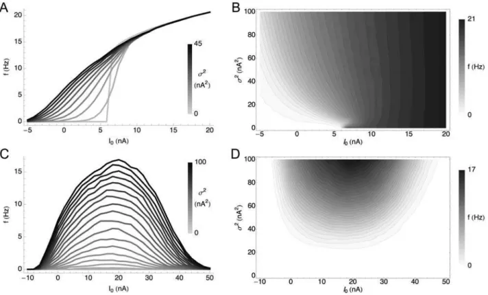
Figure 1 shows the different gain modulation behaviors of the HH and HHLS conductance-based models. For the HH model, Figure 1A, thef-Icurves in the presence of noise are similar to the noiseless case except that they are increasingly smoothed at the threshold. In contrast, Figure 1C shows that thef-Icurves of the HHLS model never converge toward each other as the noise level
increases. This case resembles that of layer 5 pyramidal neurons in rat medial prefrontal cortex [4], as well as nucleus laminaris (NL) neurons in the chick auditory brainstem and some pyramidal neurons in layer 2/3 of rat neocortex [3]. While for these layer 2/3 neurons, there is evidence that this change inf-Icurve slope may be related to the sAHP current [3], at steady state this effect can be obtained in general by tuning the maximal conductances without introducing any mechanism for spike rate adaptation [7].
Gain Modulation and Adaptation of Fixed Models For a system described by an LN model with a single feature, we derive an equation relating the slopes of the firing rate with respect to stimulus mean and variance. We then consider gain modulation in a system with multiple relevant features and derive a series of equations relating gain change to properties of the spike-triggered average and spike-triggered covariance. Throughout, we assume that the underlying system is fixed, and that its parameter settings do not depend on stimulus statistics. For example, if the model has a single exponential filter with a time constantt, we assume thatt does not change with the stimulus mean (I0) or variance (s2
). However, this does not mean that the model shows a single response pattern regardless of the statistical structure of stimuli. The sampled LN description of a nonlinear system with fixed parameters—even when the underlying model is an LN model [25]—can show interaction with the input statistics, leading to different LN model descriptions for different input parameters [19,25,27–29]. We refer to this asintrinsic adaptation.
One-Dimensional Model
An LN model is composed of its relevant features {em(t)} (m = 1,2,…,n)), which act as linear filters on an incoming stimulus, and a probability to spike given the filtered stimulus,P(spike|filtered stimulus). For a Gaussian white noise stimulus with meanI0and variances2
, the firing rate is
f I0,s2~ ð
dxPðspikejI0eezxÞpð Þx ð1Þ
wheree~Ð?
0 eð Þtdtis the time-integrated filter andxis the
mean-subtracted noise stimulus filtered by thenrelevant features.p(x) is ann-dimensional Gaussian distribution with variances2
. We refer to the Materials and Methods section for a more detailed account of the model.
For a one-dimensional model n = 1, Equation 1 can be rewritten with change of variables
f I0,s2
~
ð?
{?
dx PðspikejxÞp xð {I0eeÞ ð2Þ
Sincep(x) is Gaussian, it is also the kernel or Green’s function of a diffusion equation in terms of (x,s2) and therefore so isp(x2I0e¯) in terms of (I0,s2). In other words, we have
L Ls2{
1 2
L2 Lx2
!
p xð {I0eeÞ
~ L
Ls2{
1 2ee2
L2 LI2
0 !
p xð {I0eeÞ~0
Now operating with L Ls2{21e2 L
2
LI2 0
on both sides of the equation,
p(x2I0e¯) is the only term on the left hand side of Equation 2 that
Author Summary
depends on (I0,s2
) and therefore the right hand side of Equation 2 vanishes. Thus one finds
2e2 Lf Ls2~
L2f
LI2 0
ð3Þ
The boundary condition is given by evaluating Equation 2 as s2
R0; here the Gaussian distribution becomes a delta function
lim s2?0p x
{I0e
ð Þ~dðx{I0eÞ
and the boundary condition is given by the zero-noisef-I curve. Thus, when a model depends only on a single feature,e(t), thef-I curve with a noisy input is given by a simple diffusion-like equation, Equation 3, with a single parameter, the time integrated filter,e~Ð0?e tð Þdt, determining the diffusion constant 1/2e¯2
. Equation 3 states that the variance-dependent change in the firing rate is simply determined by the curvature of thef-Icurve. Thus, a one-dimensional system displays only a single type of noise-induced gain modulation: as in diffusion, an f-I curve is gradually smoothed and flattened as the variance increases. Given a boundary condition, such as an f-I curve for a particular variance, the family off-Irelations can be reconstructed up to a scale factor by solving Equation 3. For example, one can predict how the neuron would respond to a noise stimulus based on its output in the absence of noise. Note that the solution of Equation 3
generalizes a classical result [33] based on a binary nonlinearity to a simple closed form which applies to any type of nonlinearity.
Figure 2A and 2B show a solution of Equation 3. While this one-dimensional model is based on the simplest and most general assumptions, it provides insights into the structure of variance-dependent gain modulation. The boundary condition is an f-I curve with no noise,f = (I+0.1)1/2forI.0 and f = 0 forI#0, which imitates the general behavior of many dynamical neuron models around rheobase [34–36]. Compared with the HH conductance-based model, Equation 3 captures qualitative characteristics of the HHf-I curve despite differences due to the increased complexity of the HH model over a 1D LN model: in Figure 2A and 2B, there is a positive curvature (second derivative of firing rate with respect to current) of the f-I curve below rheobase related to the increase of the firing rate with increasing variance. In contrast, the behavior of the HHLS model cannot be described by Equation 3. Even though thef-Icurves in Figure 1C mostly have negative curvature, the firing rate keeps increasing with variance, implying that the HHLS model cannot be described by a one-dimensional LN model.
We also compared Equation 3 with the f-I curves from two commonly used simple neuron models, the leaky integrate-and-fire (LIF) model (Figure 2C), and a similar model with minimal nonlinearity, the quadratic integrate-and-fire (QIF) model [37,38] (Figure 2D). Thef-Icurves of the two models are similar but have subtle differences: in the LIF model, firing rate never decreases with noise, even though parameters were chosen to induce a large negative curvature, as shown analytically in Text S1. The QIF
Figure 1. Variance-Dependent Gain Modulation of the HH and HHLS Model.Each model is simulated as described in the Materials and Methods section. (A)f-Icurves of a standard HH model for differing 10 variances (s2) from 0 to 45 nA2. The topmost trace is the response to the highest variance. Each curve is obtained with 31 mean values (I0) ranging from25 to 20 nA. (B) The same data as (A) plotted in the (mean, variance) plane. Lighter shades represent higher firing rates. We used cubic spline interpolation for points not included in the simulated data. (C,D)f-Icurves of the HHLS model as in (A) and (B). 10 means from210 to 50 nA and 21 variances from 0 to 100 nA2are used.
model behavior is much more similar to the 1D LN model, marked by a slight decrease in firing rate at largeI0. From this perspective, the QIF is a simpler model in terms of the LN description despite the dynamical nonlinearity.
It is interesting to note that for one-dimensional models, the gain modulation given by Equation 3 depends only on the boundary condition, which implicitly describes how an input with a given mean samples the nonlinearity, but not explicitly on the details of filters or nonlinearity. An ideal differentiator, where firing rate is independent of the stimulus mean, is realized only when the filter has zero integral,e¯ = 0. This is also the criterion that would be satisfied if the filter itself were ideally differentiating. We will return to the relationship between the LN model functional description and that of thef-Icurves in the Discussion.
Multidimensional Models
Here we examine gain modulation in the case of a system with multiple relevant features. In this case, one cannot derive a single simple equation such as Equation 3. Instead, we derive relationships between the characteristics of f(I0,s) curves and quantities calculated using white noise analysis.
Fixed multidimensional models can display far more complex response patterns to different stimulus statistics than one-dimensional models, because linear components in the model can now interact nonlinearly [29]. For example, in white noise analysis, as the stimulus variance increases, the distribution of the filtered stimuli also expands and probes different regions of the nonlinear threshold structure of the model. This induces a variance-dependent rotation among the filters recovered through sampling by white noise analysis, and the
corresponding changes in the spike-triggered average, spike-triggered covariance, and the sampled nonlinearity [19].
Here, we relate parameters of the changing spike-triggered average and spike-triggered covariance description to the form of thef-Icurves. The relationships are derived by taking derivatives of each side of Equation 1 with respect toI0ands2(see Materials and Methods section). The first order in I0 establishes the relationship between the STA and the gain of thef-Icurve with respect to the mean
Llogf
LI0
~1
s2STA, STA~
ð?
0
dtSTAð Þt ð4Þ
The second order leads to a relationship between the second derivative of thef-Icurve and the covariance matrix
L2logf
LI2 0
~ 1
s4DC, DC~ ð
dtdt0DCðt,t0Þ ð5Þ
The gain with respect to the variance is
Llogf
Ls2 ~
1
2s4 TrDCzkSTAk 2
ð6Þ
where
TrDC~
ð
dtDCð Þt,t, kSTAk2~
ð
Equations 4–6 show how the nonlinear gain of anf-Icurve with respect to input mean and variance is related to intrinsic adaptation as observed through changes in the STA and STC. Note that Equations 4–6 apply to one-dimensional LN models as well. In that case, the STA has the same shape as the feature in the model, and only its magnitude varies according to the overlap integral, Equation 1, between the nonlinearity of the model and the prior stimulus. This is the same for the STC, and thus Equations 4–6 are not independent. This leads to a single form of variance gain modulation, given by Equation 3. However, in a multidimensional model, changing the stimulus mean shifts the nonlinearity in a single direction, STA, while increasing the
variance expands the prior in every direction in the stimulus space. Therefore, the overlap integral can show more diverse behaviors.
Conductance-Based Models
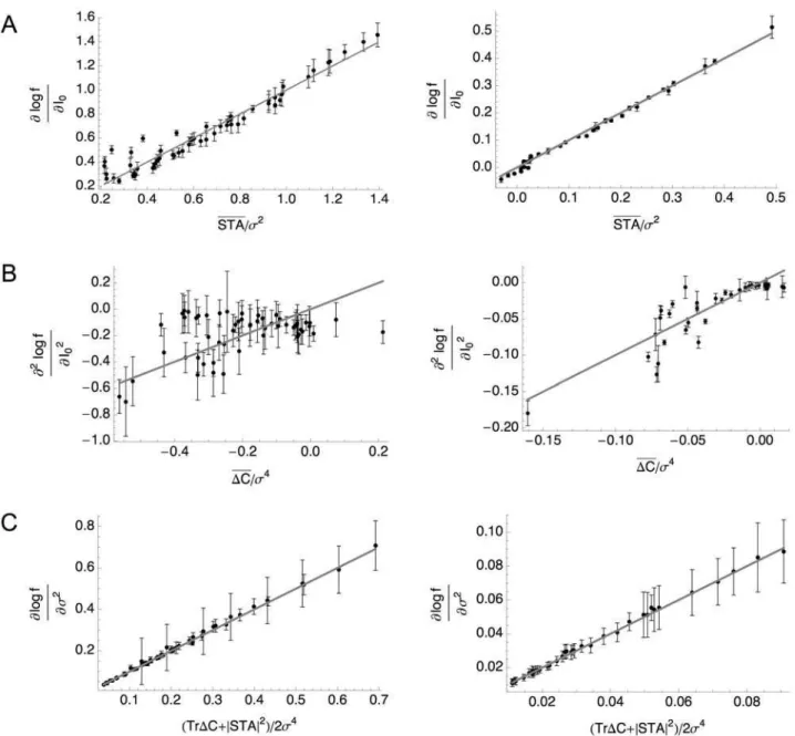
We now examine whether the gain modulation behaviors we have described can be captured by a multi-dimensional LN model. We tested this by computingf-I curves, spike-triggered averages and the spike-triggered covariance matrices for the noise-driven HH and HHLS models for a range of input statistics. Figure 3A, B, and C show the result of fitting simulation data from the HH (left) and HHLS (right) model to Equations 4, 5, and 6, respectively. The linear relationships are quite clear in Figure 3A
Figure 3. Derivatives of the Firing Rate Curves with Respect to Mean and Variance Related to Quantities Obtained by White Noise Analysis for the Standard HH (Left) and HHLS (Right) Models.Each point is calculated from the simulated data with a selected (mean, variance) input parameter pair, as described in the Materials and Methods section, and the gray lines represent our theoretical predictions, Equations 4–6, which hold when the variance dependent change inf-Icurves is only due to intrinsic adaptation. (A) Gain versus the norm of the STA, as in Equation 4. (B) Gain change versus the spike-triggered covariance term of Equation 5. (C) Change of firing rate with respect to variance versus the function of the STA and spike-triggered covariance given in Equation 6.
and 3C which show the gains with respect to mean and variance. Figure 3B involves the curvature of f-I curves, which is more difficult to calculate accurately, and shows larger errors. In every case, goodness of fit isp,1.361026
andp,5.861026
for the HH and HHLS where the upper bounds ofp-values are given by the case of Equation 5, corresponding to Figure 3B. These results show that intrinsic adaptation of the LN model predicts the form of noise-induced gain modulation for these models.
Gain Rescaling of One-Dimensional Models
Here we discuss a consequence of intrinsic adaptation for neuronal encoding of mean and variance information for a one-dimensional model. In this case, Equation 3 completely specifies intrinsic adaptation, and therefore we will focus on this case.
Our first observation is that Equation 3 is invariant under the simultaneous rescaling of the mean and standard deviation, I0RaI0, sRas, where a is an arbitrary positive number. This invariance is preserved if the solution is also a function of only a dimensionless variable I0/s, which would represent a signal-to-noise ratio if we describe the neuron’s input/output function in terms of an f-I curve at a fixed noise level s. Note that this situation is analogous to the Weber–Fechner [39,40] and Fitts’ law [41], which states that perception tends to depend on only dimensionless variables that are invariant under scaling of the absolute magnitude of stimulus [42]. However, the invariance of Equation 3 under the scaling of a stimulus does not necessarily lead to the invariance of a firing rate solution. By rewriting Equation 2 in terms of the ‘‘rescaled’’ variables, y=x/s and m=I0/s, we get
fm,s2
~ 1
ffiffiffiffiffiffi
2p p
ð
dye{ðy{meeÞ2=2f 0
ys
ee
ð7Þ
where f0(I) =P(spike|Ie¯) is an f-I curve with no noise. Thus, the scaling of f(I0,s2
) with standard deviation depends on the boundary condition,f0(I), which in principle can be any arbitrary function.
Nevertheless, in practice, the f-I curves of many dynamical neurons are not completely arbitrary but can share a simple scaling property, at least asymptotically. For example, in the QIF and many other neuron models, the f-I curve with no noise asymptotically follows a power law f0,(I02Ic)1/2 around the
rheobaseIc[34–36]. In general, iff0(I)/Iaasymptotically in such a regime, from Equation 7, the firing rate is asymptotically factorized into asdependent andm=I0/sdependent part as
fm,s2
!saFð Þm , Fð Þm~ 1ffiffiffiffiffiffi
2p p
ð
dye{ðy{meeÞ2=2ya ð8Þ
In other words, I0/s becomes an intermediate asymptoticof thef-I curves [43].
To test to what extent this scaling relationship holds in the models we have considered, we calculated therescaled relative gainof thef-Icurves, which we define as (s/f)hf/hI0=shlogf/hI0; the rescaled relative gain of Equation 8 depends only onm=I0/s, not ons. Thus, if the rescaling strictly holds, this becomes a single-valued function of the signal-to-noise ratio,I0/s, regardless of the noise levels.
We find evidence for this form of variance rescaling in the QIF, LIF, and HH models. Figure 4 shows the rescaled gains evaluated from the simulated data. The QIF and HH case, Figure 4B and 4D, match well with the solution of Equation 3, Figure 4A. In the LIF case, Figure 4C, the relative gain shows deviations at low
variance, but it approaches a variance-independent limit at large s. We also present an analytic account in Text S1. On the other hand, in Figure 4E, the HHLS model does not exhibit this form of asymptotic scaling at all. The role of the signal-to-noise ratio,I0/s, in the HHLS model appears to be quite distinct from the other models. In summary, Equation 3 predicts that one-dimensional LN models will have the tendency to decrease gain with increasing noise level. However, if thef-Icurve of a neuron is power-law-like, the resulting gain modulation will be such that the neuron’s sensitivity to mean stimulus change at various noise levels is governed only by the signal-to-noise ratio.
Discussion
In this paper, we have obtained analytical relationships between noise-dependent gain modulation off-I curves and properties of the sampled linear/nonlinear model. We have shown that gain control arises as a simple consequence of the nonlinearity of the LN model, even with no changes in any underlying parameters.
For a system described by an LN model with only one relevant feature, a simple single-parameter diffusion relationship relates the f-I curves at different variances, where the role of the diffusion coefficient is taken by the integral of the STA. This form strictly limits the possible forms of gain modulation that may be manifested by such a system. The result qualitatively describes the variance dependent gain modulation of different neuron models such as the LIF, QIF, and standard HH neuron models. Models based on dynamical spike generation, such as QIF, showed better agreement with this result than the LIF model. The QIF model case is a good example of how a nonlinear dynamical system can be mapped onto an LN model description [19,44]. The QIF model has a single dynamical equation whose subthreshold dynamics are captured approximately by a linear kernel, which takes the role of the feature; one can then determine a threshold which acts as a binary decision boundary for spiking. Thus, it is reasonable that the QIF model and the one-dimensional LN model show a similar response pattern to a noisy input. When the system has multiple relevant features, we obtain equations relating the gain with respect to the input mean and the input variance to parameters of the STA and STC. We verified these results using HH neurons displaying two different forms of noise-induced gain control.
Previous work has related different gain control behaviors to a neuron’s function as an integrator or a differentiator [3,7]. From an LN model perspective, the neuron’s function is defined by specific properties of the filter or filterse(t). An integrating filter would consist of entirely positive weights; for leaky integrators these weights will decay at large negative times. A differentiating filter implements a local subtraction of the stimulus, and so should consist of a bimodal form where the positive weights approxi-mately cancel the negative weights.
One might then ask how the system can decode the represented information. It has been proposed that statistics of the spike train might provide the information required to decode slower-varying stimulus parameters [22,45]. The possibility of distinguishing between responses to different stimulus statistics using the firing rate alone depends on the properties of thef-Icurves.
The primary focus of this work is the restricted problem of single neurons responding to driving currents, where the integrated synaptic current in an in vivo-like condition is approximated to be a (filtered) Gaussian white noise [46–50]. However, our deriva-tions can apply to arbitrary neural systems driven by white noise inputs, iff-Icurves are interpreted as tuning functions with respect
to the mean stimulus parameter. Given the generality of our results for neural systems, it would be interesting to test our results in cases where firing is driven by an external stimulus. A good candidate would be retinal ganglion cells, which are well-described by LN-type models [9,14,51–53], show adaptation to stimulus statistics on multiple timescales [23,54] and display a variety of dimensionalities in their feature space [14].
A limitation of the tests we have performed here is a restriction to the low firing rate regime where spike-triggered reverse correlation captures most of the dependence of firing probability on the stimulus. The effects of interspike interaction can be significant [16,17,55] and models with spike history feedback have
Figure 4. Rescaled Relative Gains of Variance-Dependentf-ICurves.(A) The one-dimensional LN, (B) QIF, and (C) LIF models. The same data as Figure 2 are used. (D) The standard HH model from Figure 1A and 1B. (E) The HHLS model from Figure 1C and 1D. Since the HHLS does not have a rheobase, we instead usedIcenter= 20 nA at which the variance-dependent firing rate increase is maximal.
been developed to account for this [44,51,56,57]. We have not investigated how spike history effects would impact our results.
Although evidence suggests that gain modulation by noise may be enhanced by slow afterhyperpolarization currents underlying spike frequency adaptation [3], these slow currents are not required to generate gain enhancement in simple neuron models [7,19,25–29]. While one may generate diverse types of noise-induced gain modulation only by modifying the mechanism of generating a spike independent of spike history [7], in realistic situations, slow adaptation currents are present and will affect neural responses over many timescales [58–60]. In principle, it is possible to extend our result to include these effects: f-I curves under conditions of spike frequency adaptation have been already discussed [61–63] and can be compared to LN models with spike history feedback. However, our goal here was to demonstrate the effects that can occur independent of slow adaptation currents and before such currents have acted to shift neuronal coding properties.
The suggestive form of our result for one-dimensional LN models led us to look for a representation of neuronal output that is invariant under change in the input noise level. Our motivation is based on a simple principle of dimensional analysis: the gains of the f-I curves with noise may be asymptotically described by a signal-to-noise ratio, a dimensionless variable depending only on the stimulus itself. We showed that this may occur if thef-Icurve with no noise obeys asymptotic power-law properties. Such a property has been determined to arise both from the bifurcation patterns of spike generation [31,34,35] and due to spike rate adaptation [61]. This relationship implies that the gain of the firing rate as a function of the mean should scale inversely with the standard deviation. Scaling of the gain of the nonlinear decision function with the stimulus standard deviation has been observed to some degree in a number of neural systems [10,15,22– 25,29,64–67]. Such scaling guarantees maximal transmission of information [10,22]. As we and others have proposed, a static model might suffice to explain this phenomenon [25,27], although in some cases slow adaptation currents are known to contribute [65,66].
In summary, we have presented theoretically derived relation-ships between the variance-dependent gain modulation of f-I curves and intrinsic adaptation in neural coding. In real neural systems, any type of gain modulation likely results from many different mechanisms, possibly involving long-time scale dynamics. Our results show that observed forms of gain modulation may be a result of a pre-existing static nonlinearity that reacts to changes in the stimulus statistics robustly and almost instantaneously.
Materials and Methods
Biophysical Models
We used two single compartmental models with Hodgkin– Huxley (HH) active currents. The first one is an HH model with standard parameters while the second model (HHLS) has a lower Na+and higher K+maximal conductance. The voltage changes are described by [32]
CdV
dt ~{ggLðV{ELÞ{ggNam
3h V{E Na
ð Þ{ggKn4ðV{EKÞzI tð Þ
and the activation variablesm,n, andhbehave according to
tzð ÞV
dz
dt~zz Vð Þ{z, tz~ 1
azzbz
, zz~ az
azzbz
, z~m,n,h
where
am~
0:1ðVz40Þ
1{exp½{0:1ðVz40Þ, bm~4 exp½{0:0556ðVz65Þ, ah~0:07 exp 0½ :05ðVz65Þ, bh~
1
1zexp½{0:1ðVz35Þ, an~
0:01ðVz55Þ
1{exp½{0:1ðVz55Þ, bn~0:125 exp½{0:0125ðVz65Þ
The voltageVis in millivolts (mV).
For the HH model, the conductance parameters are g¯K= 36 mS/cm2 and g¯Na= 120 mS/cm2. The HHLS model has g¯K= 41 mS/cm2 andg¯Na= 79 mS/cm2. All other parameters are common to both models. The leak conductance isg¯L= 0.3 mS/ cm2and the membrane capacitance per areaCis 1mF/cm2. The reversal potentials are EL=254.3 mV, ENa= 50 mV, and EK=277 mV. The membrane area is 1023cm2, so that a current density of 1mA/cm2corresponds to a current of 1 nA.
All simulations of these models were done with the NEURON simulation environment [68]. Gaussian white noise currents with various means and variances are generated with an update rate of 5 kHz (dt= 0.2 ms) and delivered into the model via current clamp. For thef-I curves, we simulated 4 min of input for each mean and variance pair. The whole procedure was repeated five times to estimate the variance of thef-Irelationship,srepeat.
We ran another set of simulations for reverse correlation analysis and collected about 100,000 spikes for each stimulus condition. The means and variances of the Gaussian noisy stimuli were chosen such that the mean firing rate did not exceed 10 Hz, and we selected eight means and seven variances for the HH model, and nine means and four variances for the HHLS model.
Integrate-and-Fire-Type Models
In addition to the conductance-based model, we investigated the behavior of two heuristic model neurons driven by a noisy current input. Each model consists of a single dynamical equation describing voltage fluctuations of the form
CdV
dt ~L Vð ÞzI tð Þ
The first model is a leaky integrate-and-fire (LIF) model [69,70], for which L(V) =2gL(V2EL). We used the parameters gL= 2, EL= 0, andC= 1. Since this choice ofL(V) cannot generate a spike, we additionally imposed a spiking threshold Vth= 1 and reset voltageVreset=23.
The second is a quadratic integrate-and-fire (QIF) model [31,37,38], for which L(V) =gL(V2EL)(V2Vth)/DV where DV=Vth2EL.0. We used gL= 0.5, EL= 0, Vth= 0.1, and C= 1. In this model, the voltageVcan increase without bound; such a trajectory is defined to be a spike if it crosses Vspike= 5. After spiking, the system is reset toVreset= 0.
Linear/Nonlinear Model
We use the linear/nonlinear (LN) cascade model framework to describe a neuron’s input/output relation. We will focus on the dependence of the firing rate of a fixed LN model on the mean and variance of a Gaussian white noise input.
We will take the driving input to beI(t) =I0+j(t) whereI0is the mean andj(t) is a Gaussian white noise with variances2
and zero mean. The linear part of the model selects, by linear filtering, a subset of the possible stimuli probed by I(t). That subset is expressed asnrelevant features {em(t)}, (m= 1,2,…,n). Interpreted as vectors, the components of any stimulus that are relevant to changing the firing rate can be expressed in terms of projections onto these features. The firing rate of the model for a given temporal sequenceI(t) depends only ons, the input filtered by the nrelevant features. Thus the firing rate from the given stimulus depends on the convolution of the input with allnfeatures and can be written asP(spike|s=I0e¯+x) where
eem~
ð?
0
dt emð Þt, xm~
ð?
0
dt emð Þtjðt{tÞ
SinceI(t) is white noise with stationary statistics, the projectionsxm can be taken to be stationary random variables chosen from a Gaussian distribution at eacht.
Given the filtered stimulus, a nonlinear decision function P(spike|I0e¯+x) generates the instantaneous time-varying firing rate. For a specified model and stimulus statistics, the mean firing ratef(I0,s2
) =P(spike) is simply
f I0,s2~ ð
dsPðspikejsÞPð Þs ~
ð
dxPðspikejI0eezxÞpð Þ ðx 9Þ
where
pð Þx ~ 1
2ps2 ð Þp=2
:exp { 1
2s2k kx 2
Equation 9 describes anf-Icurve of the model in the presence of added noise with variances2
. The slope orgainof the firing rate with respect to mean or variance can be computed if P(spike|I0e¯+x) is known. However, the gains can be also obtained in terms of the first and second moments ofP(spike|I0e¯+x), which can be measureddirectlyby reverse correlation analysis.
Reverse Correlation Analysis
We used spike-triggered reverse correlation to probe the computation of the model neurons through an LN model. We collected about 100,000 spikes and corresponding ensembles of spike triggered stimulus histories in a 30 ms long time window preceding each spike.
From the triggered input ensembles, we calculated spike-triggered averages (STAs) and spike-spike-triggered covariances (STCs). The STA is simply the average of the set of stimuli that led to spikes subtracted from the mean of the ‘‘prior’’ stimulus distribution, the distribution of all stimuli independent of spiking output
STAð Þt ~SI tspike{tTspike{SITprior~Sjtspike{tTspike ð10Þ
Therefore, one may consider only the noise part of the zero mean stimulus.
When computing the STC, the prior’s covariance is subtracted
DC t,tð 0Þ~Cspike{Cprior
~Sjtspike{t{STAð Þt j tspike{t0
{STAð Þt0
Tspike{Cprior ð11Þ
Statistical Analysis
In calculating the slope and curvature of thef-Icurves, we used 6–10 degree polynomial fitting of the f-I curves, where in any single case, the lowest degree was used which provided both a good fit and smoothness. From the fitting procedure, we obtained the standard deviation of the residuals,sfit. This was repeated five times forf-I curves computed using different noise samples, and from this we computed srepeat, the standard deviation of each computed slope and curvature. We estimated the total error of our calculation as stotal= (srepeat2+sfit2)1/2. In practice, srepeat was always greater thansfitby an order of magnitude. Thisstotalwas used for the error bars in Figure 3.
To evaluate the goodness of fit in Figure 3, we used the Pearson x2
test by using the reducedx2 statistic
x2~XðO{EÞ
2
s2 total
where O and E represent the right and left hand sides of Equations 4–6, respectively. From this, thep-values are estimated from the cumulative density function of thex2
distribution,Q(x2 / k,k). The degree of freedom isk= 54 andk= 34 for the HH and HHLS, respectively.
Derivation of Equations 4–6
We first present two key identities: the first one, which depends on the form ofshaving additive mean and noise components, is a change of variables for the gradient ofP(spike|x+I0e¯)
LPðspikejxzI0eeÞ
LI0
~X
m eem
LPðspikejxzI0eeÞ
Lxm ð12Þ
Secondly, whenxis a Gaussian random variable with zero mean and variances2
, by using integration by parts in can be seen that any functionF(x) satisfies
SF0ð Þx T~1
s2SxF xð ÞT ð13Þ
SF00ð Þx T~ 1
s2S½xF xð Þ ’
T{ 1
s2SF xð ÞT
~ 1
s4Sx 2F x
ð ÞT{ 1
s2SF xð ÞT
Llogf
LI0
~1
f
Lf
LI0
~1
f
X
m eemS
L
LxmPðspikejxzI0eeÞTx
~ 1
s2:
1 f
X
m
eemSxmPðspikejxzI0eeÞTx
ð14Þ
The second order is given by
L2logf
LI2 0
~1
f
L2f
LI2 0
{1
f2
Lf
LI0
2
,
L2f
LI2 0
~X
m,n eemeenS
L Lxm
L
LxnPðspikejxzI0eeÞTx
~1
s4 X
m,n
eemeenS xmxn{s2dmn
PðspikejxzI0eeÞTx, ð15Þ
wheredmnis a Kronecker delta symbol. The gain with respect to variance is
Lf
Ls2~{
n 2s2fz
1 2s4
X
m
Sx2
mPðspikejxzI0eeÞTx
~ 1
2s4 X
m
S x2
m{s2
PðspikejxzI0eeÞTx
ð16Þ
Now, we show how the right hand sides of Equations 14–16 correspond to the STA and the STC. Given a Gaussian white noise signalj(t), we can split it asj=jI+jH, wherejIbelongs to
the space spanned by our basis features {em}, and therefore relevant to spiking.jHis the orthogonal or irrelevant part.jIcan
be written as
j
jjð Þt~e:x~ X
m
xmem, xm~
ð?
0
dt emð Þtjðt{tÞ
Again,xis a Gaussian variable from a distribution Equation 9.
The STA is
STA~SjTspike~Sj jjTspike~
ð
dnxðe:xÞPðxzI0eejspikeÞ
sincejHis irrelevant and does not make any contribution. Here
we use Bayes theorem
PðspikejxzI0eeÞ
PðspikeÞ ~
PðxzI0eejspikeÞ
PðxzI0eeÞ
As in Equation 9, P(s=x+I0e¯) =p(x), and therefore the STA becomes
STA~
ð
dnxðe:xÞPspike xzI0ee j
ð Þ
PðspikeÞ pð Þx
~1
f
X
m
emSxmPðspikejxzI0eeÞTx
Comparing this result with Equation 14, we obtain Equation 4. A similar calculation for the second order [19] shows
DC t,tð 0Þ~1
f
X
m,n
emð Þtenð Þt0 S xmxn{s2dmn
PðspikejxzI0eeÞTx
{STAð Þt :STAð Þt0
This result, combined with Equations 15 and 16, leads to Equations 5 and 6, respectively.
Supporting Information
Text S1. Firing Rate of the LIF Model with Noisy Stimuli. Found at: doi:10.1371/journal.pcbi.1000119.s001 (0.09 MB DOC)
Author Contributions
Conceived and designed the experiments: SH. Analyzed the data: SH. Contributed reagents/materials/analysis tools: BL. Wrote the paper: SH BL AF. Derived the equations: SH.
References
1. Chance FS, Abbott LF, Reyes AD (2002) Gain modulation from background synaptic input. Neuron 35: 773–782.
2. Fellous JM, Rudolph M, Destexhe A, Sejnowski TJ (2003) Synaptic background noise controls the input/output characteristics of single cells in an in vitro model of in vivo activity. Neuroscience 122: 811–829.
3. Higgs MH, Slee SJ, Spain WJ (2006) Diversity of gain modulation by noise in neocortical neurons: regulation by the slow afterhyperpolarization conductance. J Neurosci 26: 8787–8799.
4. Arsiero M, Lu¨scher HR, Lundstrom BN, Giugliano M (2007) The impact of input fluctuations on the frequency–current relationships of layer 5 pyramidal neurons in the rat medial prefrontal cortex. J Neurosci 27: 3274–3284. 5. Prescott SA, Koninck YD (2003) Gain control of firing rate by shunting
inhibition: roles of synaptic noise and dendritic saturation. Proc Natl Acad Sci USA 100: 2076–2081.
6. Prescott SA, Ratte´ S, De Koninck Y, Sejnowski TJ (2006) Nonlinear interaction between shunting and adaptation controls a switch between integration and coincidence detection in pyramidal neurons. J Neurosci 26: 9084–9097. 7. Lundstrom BN, Hong S, Fairhall AL (2008) Two computational regimes of a
single-compartment neuron separated by a planar boundary in conductance space. Neural Comput 20: 1239–1260.
8. Victor J, Shapley R (1980) A method of nonlinear analysis in the frequency domain. Biophys J 29: 459–483.
9. Meister M, Berry II MJ (1999) The neural code of the retina. Neuron 22: 435–450.
10. Brenner N, Bialek W, de Ruyter van Steveninck R (2000) Adaptive rescaling maximizes information transmission. Neuron 26: 695–702.
11. Simoncelli EP, Paninski L, Pillow J, Schwartz O (2004) Characterization of neural responses with stochastic stimuli. In: Gazzaniga M, ed. The Cognitive Neurosciences. 3rd edition. Cambridge (Massachusetts): MIT Press. 12. Rust NC, Schwartz O, Movshon JA, Simoncelli EP (2005) Spatiotemporal
elements of macaque V1 receptive fields. Neuron 46: 945–956.
13. Stanley GB, Lei FF, Dan Y (1999) Reconstruction of natural scenes from ensemble responses in the lateral geniculate nucleus. J Neurosci 19: 8036–8042. 14. Fairhall AL, Burlingame CA, Narasimhan R, Harris RA, Puchalla JL, et al. (2006) Selectivity for multiple stimulus features in retinal ganglion cells. J Neurophysiol 96: 2724–2738.
15. Maravall M, Petersen RS, Fairhall AL, Arabzadeh E, Diamond ME (2007) Shifts in coding properties and maintenance of information transmission during adaptation in barrel cortex. PLoS Biol 5: e19. doi:10.1371/journal. pbio.0050019.
16. Agu¨era y Arcas B, Fairhall AL (2003) What causes a neuron to spike? Neural Comput 15: 1715–1749.
18. Slee SJ, Higgs MH, Fairhall AL, Spain WJ (2005) Two-dimensional time coding in the auditory brainstem. J Neurosci 25: 9978–9988.
19. Hong S, Agu¨era y Arcas B, Fairhall AL (2007) Single neuron computation: from dynamical system to feature detector. Neural Comput 19: 3133–3172. 20. Atick JJ (1992) Could information theory provide an ecological theory of sensory
processing? Network (Bristol, England) 3: 213–251.
21. Theunissen FE, Sen K, Doupe AJ (2000) Spectral-temporal receptive fields of nonlinear auditory neurons obtained using natural sounds. J Neurosci 20: 2315–2331.
22. Fairhall A, Lewen G, Bialek W, de Ruyter van Steveninck RR (2001) Efficiency and ambiguity in an adaptive neural code. Nature 412: 787–792.
23. Baccus SA, Meister M (2002) Fast and slow contrast adaptation in retinal circuitry. Neuron 36: 909–919.
24. Nagel KI, Doupe AJ (2006) Temporal processing and adaptation in the songbird auditory forebrain. Neuron 51: 845–859.
25. Gaudry KS, Reinagel P (2007) Benefits of contrast normalization demonstrated in neurons and model cells. J Neurosci 27: 8071–8079.
26. Rudd ME, Brown LG (1997) Noise adaptation in integrate-and-fire neurons. Neural Comput 9: 1047–1069.
27. Paninski L, Lau B, Reyes AD (2003) Noise-driven adaptation: in vitro and mathematical analysis. Neurocomputing 52: 877–883.
28. Yu Y, Lee TS (2003) Dynamical mechanisms underlying contrast gain control in single neurons. Phys Rev E 68: 011901.
29. Borst A, Flanagin VL, Sompolinsky H (2005) Adaptation without parameter change: dynamic gain control in motion detection. Proc Natl Acad Sci USA 102: 6172–6176.
30. Hodgkin AL (1948) The local electric changes associated with repetitive action in a non-medullated axon. J Physiol 107: 165–181.
31. Izhikevich EM (2006) Dynamical Systems in Neuroscience: The Geometry of Excitability and Bursting. Cambridge (Massachusetts): MIT Press.
32. Hodgkin AL, Huxley AF (1952) A quantitative description of membrane current and its application to conduction and excitation in nerve. J Physiol 463: 391–407.
33. Spekreijse H, Reits D (1982) Sequential analysis of the visual evoked potential system in man: nonlinear analysis of a sandwich system. Ann N Y Acad Sci 388: 72–97.
34. Ermentrout GB (1994) Reduction of conductance-based models with slow synapses to neural nets. Neural Comput 6: 679–695.
35. Rinzel JM, Ermentrout GB (1989) Analysis of neuronal excitability. In: Koch C, Segev I, eds. Methods in Neuronal Modeling: From Synapses to Networks. Cambridge (Massachusetts): MIT Press. pp 135–170.
36. Hoppensteadt F, Izhikevich EM (1997) Weakly Connected Neural Nets. Berlin: Springer-Verlag.
37. Ermentrout GB, Kopell N (1986) Parabolic bursting in an excitable system coupled with a slow oscillation. SIAM J Appl Math 4: 233–253.
38. Ermentrout B (1996) Type I membranes, phase resetting curves, and synchrony. Neural Comput 8: 979–1001.
39. Weber EH (1834) De Pulsu, Resorptione, Auditu et Tactu. Annotiones Anatomicae et Physiologicae. Lipsiae: Koehler.
40. Fechner G (1966) Elements of Psychophysics. New York: Holt, Rinehart and Winston.
41. Fitts PM (1954) The information capacity of the human motor system in controlling the amplitude of movement. J Exp Psychol 47: 381–391. 42. Stevens SS (1986) Psychophysics: Introduction to Its Perceptual, Neural, and
Social Prospects. Piscataway (New Jersey): Transaction Publishers. 43. Barenblatt GI (2003) Scaling. Cambridge, UK: Cambridge University Press. 44. Gerstner W, Kistler W (2002) Spiking Neuron Models: Single Neurons,
Populations, Plasticity. Cambridge, UK: Cambridge University Press.
45. Lundstrom BN, Fairhall AL (2006) Decoding stimulus variance from a distributional neural code of interspike intervals. J Neurosci 26: 9030–9037. 46. Gerstein GL, Mandelbrot B (1964) Random walk models for the spike activity of
a single neuron. Biophys J 4: 41–68.
47. Bryant HL, Segundo JP (1976) Spike initiation by transmembrane current: a white-noise analysis. J Physiol 260: 279–314.
48. Mainen ZF, Sejnowski TJ (1995) Reliability of spike timing in neocortical neurons. Science 268: 1503–1506.
49. Destexhe A, Pare´ D (1999) Impact of network activity on the integrative properties of neocortical pyramidal neurons in vivo. J Neurophysiol 81: 1531–1547.
50. Rudolph M, Destexhe A (2003) Characterization of subthreshold voltage fluctuations in neuronal membranes. Neural Comput 15: 2577–2618. 51. Keat J, Reinagel P, Reid RC, Meister M (2001) Predicting every spike: a model
for the responses of visual neurons. Neuron 30: 803–817.
52. Chichilnisky EJ (2001) A simple white noise analysis of neuronal light responses. Network (Bristol, England) 12: 199–213.
53. Pillow JW, Paninski L, Uzzell VJ, Simoncelli EP, Chichilnisky EJ (2005) Prediction and decoding of retinal ganglion cell responses with a probabilistic spiking model. J Neurosci 25: 11003–11013.
54. Smirnakis SM, Berry MJ, Warland DK, Bialek W, Meister M (1997) Adaptation of retinal processing to image contrast and spatial scale. Nature 386: 69–73. 55. Pillow JW, Simoncelli EP (2003) Biases in white noise analysis due to
non-Poisson spike generation. Neurocomputing 52–54: 109–115.
56. Truccolo W, Eden UT, Fellows MR, Donoghue JP, Brown EN (2005) A point process framework for relating neural spiking activity to spiking history, neural ensemble, and extrinsic covariate effects. J Neurophysiol 93: 1074–1089. 57. Paninski L, Pillow J, Lewi J (2006) Statistical models for neural encoding,
decoding, and optimal stimulus design. Prog Brain Res 165: 493–507. 58. Schwindt PC, Spain WJ, Foehring RC, Stafstrom CE, Chubb MC, et al. (1988)
Multiple potassium conductances and their functions in neurons from cat sensorimotor cortex in vitro. J Neurophysiol 59: 424–449.
59. Spain WJ, Schwindt PC, Crill WE (1991) Two transient potassium currents in layer V pyramidal neurones from cat sensorimotor cortex. J Physiol 434: 591–607.
60. La Camera G, Rauch A, Thurbon D, Lu¨scher HR, Senn W, et al. (2006) Multiple time scales of temporal response in pyramidal and fast spiking cortical neurons. J Neurophysiol 96: 3448–3464.
61. Ermentrout B (1998) Linearization of F-I curves by adaptation. Neural Comput 10: 1721–1729.
62. Benda J, Herz AVM (2003) A universal model for spike-frequency adaptation. Neural Comput 15: 2523–2564.
63. La Camera G, Rauch A, Lu¨scher HR, Senn W, Fusi S (2004) Minimal models of adapted neuronal response to in vivo-like input currents. Neural Comput 16: 2101–2124.
64. Kim KJ, Rieke F (2001) Temporal contrast adaptation in the input and output signals of salamander retinal ganglion cells. J Neurosci 21: 287–299. 65. Arganda S, Guantes R, de Polavieja GG (2007) Sodium pumps adapt spike
bursting to stimulus statistics. Nat Neurosci 10: 1467–1473.
66. Diaz-Quesada M, Maravall M (2008) Intrinsic mechanisms for adaptive gain rescaling in barrel cortex. J Neurosci 28: 696–710.
67. Ringach DL, Malone BJ (2007) The operating point of the cortex: neurons as large deviation detectors. J Neurosci 27: 7673–7683.
68. Hines ML, Carnevale NT (1997) The NEURON simulation environment. Neural Comput 9: 1179–1209.
69. Knight BW (1972) Dynamics of encoding in a population of neurons. J Gen Physiol 59: 734.