Model Vestibular Nuclei Neurons Can Exhibit a Boosting Nonlinearity Due to an Adaptation Current Regulated by Spike-Triggered Calcium and Calcium-Activated Potassium Channels.

Model Vestibular Nuclei Neurons Can Exhibit

a Boosting Nonlinearity Due to an

Adaptation Current Regulated by

Spike-Triggered Calcium and Calcium-Activated

Potassium Channels

Adam D. Schneider*

Physics, McGill University, Montreal, Quebec, Canada

*adam.schneider@mail.mcgill.ca

Abstract

In vitrostudies have previously found a class of vestibular nuclei neurons to exhibit a bidi-rectional afterhyperpolarization (AHP) in their membrane potential, due to calcium and cal-cium-activated potassium conductances. More recentlyin vivostudies of such vestibular neurons were found to exhibit a boosting nonlinearity in their input-output tuning curves. In this paper, a Hodgkin-Huxley (HH) type neuron model, originally developed to reproduce thein vitroAHP, is shown to produce a boosting nonlinearity similar to that seenin vivofor increased the calcium conductance. Indicative of a bifurcation, the HH model is reduced to a generalized integrate-and-fire (IF) model that preserves the bifurcation structure and boosting nonliearity. By then projecting the neuron model’s phase space trajectories into 2D, the underlying geometric mechanism relating the AHP and boosting nonlinearity is revealed. Further simplifications and approximations are made to derive analytic expres-sions for the steady steady state firing rate as a function of bias current,μ, as well as the

gain (i.e. its slope) and the position of its peak atμ=μ*. Finally, although the boosting

non-linearity has not yet been experimentally observedin vitro, testable predictions indicate how it might be found.

Introduction

A primary goal of computational neuroscience is to understand the nature of the“neural code” with which sensory information is represented and processed by successive stages of neurons in the nervous system. Sensory neurons were first shown to encode stimulus features such as intensity, in the rate at which they fire action potentials. Accordingly, sensory neurons are often characterized by“tuning curves”, which provide a map from a particular stimulus param-eter (such as intensity) to the neurons output firing rate [1]. Although linear transformations are known to preserve information, nonlinear transformations are essential for the selective

PLOS ONE | DOI:10.1371/journal.pone.0159300 July 18, 2016 1 / 27

a11111

OPEN ACCESS

Citation:Schneider AD (2016) Model Vestibular Nuclei Neurons Can Exhibit a Boosting Nonlinearity Due to an Adaptation Current Regulated by Spike-Triggered Calcium and Calcium-Activated Potassium Channels. PLoS ONE 11(7): e0159300. doi:10.1371/ journal.pone.0159300

Editor:Jonathan David Touboul, College de France, FRANCE

Received:March 8, 2016

Accepted:June 30, 2016

Published:July 18, 2016

Copyright:© 2016 Adam D. Schneider. This is an open access article distributed under the terms of the Creative Commons Attribution License, which permits unrestricted use, distribution, and reproduction in any medium, provided the original author and source are credited.

Data Availability Statement:All relevant data are within the paper.

Funding:The author has no support or funding to report.

coding of particular stimulus features, as well as using a neurons full information transmission capacity [2]. In the vestibular system, for example, semicircular canal afferents have long been known to primarily encode angular head velocity through firing rate modulations that vary lin-early with increasing stimulus amplitude until saturation or rectification occurs [3], whereupon the neuron has reached its maximum or minimum firing rate, respectively. More recently how-ever,in vivostudies have shown that neurons in the medial vestibular nuclei (VN) exhibit a boosting nonlinearity in their input-output tuning curves (i.e. firing rate output, versus stimu-lus, afferent, or bias current input; a.k.a. tuning or f-I curve) [4]. This boosting nonlinearity is characterized by a linear region with a small positive slope for low afferent input currents, and a linear region with higher positive slope for larger afferent inputs, rather than the more com-mon occurrence of a higher slope at low bias currents.In vitrostudies, on the other hand, mea-sure the membrane potential time course and have developed a conductance based Hodgkin-Huxley-type VN model, with voltage-activated calcium and calcium-activated potassium chan-nels that produce a specific bidirectional afterhyperpolarization (AHP) [5,6]. In this paper, a simpler version of this model is shown to produce a boosting nonlinearity similar to that observed experimentallyin vivo[4], for increased calcium conductances,gCa, which acts as a bifurcation parameter. In order to shed some light on the underlying mechanisms responsible, a simplified integrate-and-fire (IF) type model is created that is more analytically tractable but preserves the bifurcation structure and boosting nonlinearity under investigation.

It requires a system with at least two variables with nonlinear dynamics to produce action potentials with sodium and potassium currents; the simplicity of IF models is that they replace these spike generating ion channels, with a simpler boundary condition that takes the voltage from threshold back to a reset value [7]. Single variable (i.e. membrane voltage, V) IF models can then be made to have more realistic subthreshold dynamics (which will be required to pro-duce the AHP) by adding back a voltage dependent function,ψ(V). Alinear“leak”term (giving an LIF) allows the membrane to return to a given resting potential in the absence of stimula-tion, and aquadraticterm (giving a QIF) will also add a depolarizing up stroke in the voltage preceding action potentials to better match their shape. A combined linear and exponential function (giving an EIF), has been shown to better fit experimental data [8–10], at a sacrifice to its analytic tractability. Such IF models can be further generalized to include any extra currents, which may require additional dynamic gating variables, such as spike-triggered adaptation cur-rents (often denoted by W) which serve to decrease V. However, such additional variables also require additional reset conditions, for the change in W upon spiking. The spiking dynamics of such 2-variable (i.e. V,W) adaptive IF models have been extensively studied [11–13], showing that they can produce a variety of spiking behaviors including a similar boosting nonlinearity and a unidirectional AHP [14], for certain parameter combinations.

In this paper, a Hodgkin Huxley (HH) type spiking VN neuron model is reduced to a QIF model generalized to include the calcium and calcium-activated potassium currents, which preserves the bifurcation structureand the boosting nonlinearity observed in the original HH model. The spiking trajectories of the resulting 3-variable adaptive QIF model are then pro-jected into the 2D V-W phase space, revealing an intuitive geometrical picture linking the AHP phase space trajectories with the low gain region of the boosting nonlinearity. Simplifying the models reset conditions and making some additional assumptions, allows for an analytic approximation for the steady state firing rate and its gain (i.e. f-I curve slope) across a similar boosting nonlinearity, as well as the bias current at which the gain is peaked,μ=μ. Although this boosting nonlinearity in the f-I curve of VN neurons has not be experimentally observed

in vitro, the link with the AHP generation provides the testable prediction that it should be found in the transition to increased bias currents where the AHP no longer occurs.

Results

HH model produces boosting nonlinearity with AHP and bifurcation

through bursting separating low and high gain regions

Fig 1Ashows a schematic of the conductance based Hodgkin-Huxley (HH) type model (defined by Eqs (4) and (5) inModels and Methods), which was simulated with different cal-cium conductance strengths,gCa, over a range of constant bias current injections,μ. Although the full HH model has 4 dynamical variables, example traces of the voltage,V, as well as the gating variable,x, and calcium concentration,C, are shown for different bias currents, and a specific calcium conductance inFig 1B–1D. The dashed green lines indicate a voltage thresh-old, crossings of which are defined to be spike times, which in turn define a sequence of inter-spike-intervals (ISIs). In panels B and D, red circles indicate regions immediately after spiking that are shown in insets, indicating that the specific AHP in which the voltage changes direc-tions twice, occurs at low bias but not high bias currents. At each bias current value, 1/ISI can be used to give the firing rate, which can be averaged over possibly different ISIs in the case of bursting solutions, such as shown inFig 1C. These average firing rates are plotted as a function of bias current (known as an f-I curve) inFig 1E, also with the individual 1/ISIs of the bursts as dots. A boosting nonlinearity (i.e. an increase in gain with an increase in bias current) can be seen to occur for the two highestgCavales (cyan and magenta curves), while for the intermedi-ategCavalue (red curve) the effect is to linearize the f-I curve by reducing the gain at the onset of spiking nearμ= 0.

It can also be seen that when the boosting nonlinearity occurs, stable limit cycles of a single ISI are present for sufficiently low or high bias currents, while stable bursting limit cycles (i.e. 2-spk burst, 3-spk burst) appear for intermediate bias current values where the gain (i.e. f-I slope) changes across the boosting nonlinearity. This bifurcation through bursting is character-ized by plotting ISI return maps at various bias currents across the bursting region, as are shown inFig 1FforgCa= 0.6. From the top right panel stable 2-spk bursting can be seen to transition to stable 3-spk bursting in the lower left panel, before returning to a stable 1-spk limit cycle at higher biases. This appears to be a global“period adding”bifurcation through bursting, however, analysis of the bursting mechanism is beyond the scope of this paper which aims to understand the change in gain across the boosting nonlinearity. In order to simplify the model and isolate the mechanism underlying this boosting nonlinearity, this HH model was reduced to an analytically tractable integrate-and-fire (IF) type model, which preserves both the boosting nonlinearity and period adding bifurcation.

QIF reduction of HH model can preserve subthreshold bifurcation

structure, boosting nonlinearity, and bifurcation through bursting

To understand the mechanism underlying the HH model’s boosting nonlinearity, a reduced integrate-and-fire (IF) type model is generated, that is analytically tractable yet preserves the boosting nonlinearity and underlying bifurcation structure. This was done by replacing the gat-ing variable,n, and related spike generating currents by a nonlinear function,ψ(V), with an additional voltage threshold and reset mechanism, as described inModels and Methods. The model’s bifurcation structure can be found by calculating the fixed points at each different bias current, which are defined by the zeros of the functionH1(V,n,x,C) (seeModels and

time series inFig 1B–1D. These curves are shifted up and down withμand the zero crossings correspond to the HH model’s fixed points, with their stability calculated viaEq (7). For suffi-ciently low bias currents, there are three fixed points and the system does not spike spontane-ously. Asμis increased the curve is shifted upwards and eventually the two lower fixed points annihilate, generally resulting in the onset of spiking via a saddle-node bifurcation. However, its is possible for spiking to begin via a Hopf bifurcation, before the two subthreshold fixed points have been annihilated. The fixed point bifurcation diagrams are plotted as a function of bias current for each of the non-zero calcium conductances inFig 2B, with red dots indicating stable fixed points, and black dots indicating unstable fixed points. The blue lines indicate the maximum and minimum values of the spiking limit cycles, and the onset bifurcation is indi-cated by a green star for a saddle-node and a green x for an Hopf bifurcation. In the case of the Hopf, the point at which the two remaining unstable subthreshold fixed points annihilate is indicated by cyan stars, which can also be seen to roughly coincide with the region of the burst-ing solutions. It would appear that the burstburst-ing and boostburst-ing nonlinearity are closely related to the subthreshold fixed point bifurcation structure, which should be preserved in a reduced IF model.

Although and exponential-IF (EIF) model could provide a better fit toH1(V,n,x,C) in

the subthreshold region indicated inFig 2A, a quadratic-IF (QIF) captures the essential local minimum between threshold and reset necessary to reproduce the two subthreshold fixed points, and has the advantage of being analytically tractable. Although a cubic term could reproduce the entire‘S’shape and high voltage FP, it lies above the voltage threshold and can be ignored for our purposes. The two QIF model parameters,g2andV2, can be related to the

HH model parameters by linearizing the nonlinear functions inEq (6)and keeping only terms to second order inV, as inEq (12). However, simply choosing values ofg2= 0.1 andV2=−50

provides a sufficiently good approximation to reproduce the desired phenomena, as can be seen from the resulting functionF1(V,x,C)Eq (10)plotted inFig 2C, and bifurcation

dia-grams inFig 2D.

The QIF model, defined byEq (8)inModels and Methods, additionally requires an artificial spike waveform to activate the calcium current gating variable,x, as described byEq (9). The resulting f-I curves for this QIF model are shown inFig 2E, and can be seen to exhibit the desired boosting nonlinearities, as well as the bursting, similarly to the HH model (although for slightly different values ofgCa). In addition, this QIF model exhibits the same period adding bifurcation through bursting as the HH model, as shown by the QIF models ISI return maps (compare Figs2Fand1F). Although the QIF model reproduces the boosting nonlinearity, it also reproduces the same bursting patterns; does this mean that the bursting is necessary to cre-ate a boosting nonlinearity?

Fig 1. Calium and calcium-activated potassium currents induce boosting nonlinearity, AHP, and bifurcation through bursting.(A) A schematic indicating that the neuron model of a vestibular nuclei neuron with conductance based ion channels as described inModels and Methods Eq (5), as well as a constant current injection, which drive the membrane voltage, the“recorded”model output, to generate action potentials. (B-D) Example time series of the simulated membrane voltage, with calcium gating variable,x, and calcium concentration,C, below. Insets show zoom of region preceding spikes either with or without an AHP. Dashed green lines indicate the voltage threshold at which spike times are said to occur. Examples correspond togCa= 0.6, for the bias current values indicated by the numbered yellow circles in panel E. (E) The firing rate as a function of constant bias current injection, or“f-I curve”. Colored lines correspond to the average 1/ISIs for the calcium conductance values indicated, with the colored dots indicating each 1/ISI value of the bursting solutions (i.e. panel C). (F) ISI return maps for four example bias currents withgCa= 0.6, showing how the stable limit cycle (μ= 18) destabilizes into stable 2-spk bursting (μ= 19), and then 3-spk bursting (μ= 22), and back to a stable

single spike limit cycle (μ= 22.5). Red dots indicate the mean ISI.

Does boosting require bursting?

It would appear the the boosting nonlinearity and bursting, depend intimately on the underly-ing subthreshold bifurcation which occurs near the onset of burstunderly-ing (seeFig 3A, red Xs). How-ever, these results actually depend significantly on the artificial spike shape used, which defines the reset conditions but does not effect the subthreshold bifurcation structure shown inFig 2D. The resulting reset condition can be thought of as the amount by which the gating variables change,ΔxandΔC, plotted inFig 3B, or the reset values themselves,xresetandCreset, plotted in

Fig 3C. Are the changes in these reset values with bias current in fact necessary for the model to produce the boosting nonlinearity or bursting? This question can be answered by simplify-ing the QIF model in these two different ways, choossimplify-ing fixed values forΔxandΔC,orforxreset andCreset. The resulting f-I curves for each case are shown inFig 3D and 3E. In both cases some degree of the boosting nonlinearity can be seen, with a similar bursting occurring in D, but not in E, confirming that one can in fact achieve boosting without bursting.

To understand what is going on, one can think of the QIF model’s 3D phase space inV,x, andC. The voltage is bound by the reset and threshold, starting atVresetwith particularxreset andCresetvalues, and evolving in time until it reachesVth. The possible trajectories through this 3D phase space cannot intersect, and are all defined by the system ofEq (8), which also defines the subthreshold bifurcation structure. It is how the gating variables are reset that regulates bursting; if the gating variables are changed by a fixed amount at reset, then they must also change by an equal and opposite amount during their phase space trajectory in order to be reset back onto the same trajectory. Otherwise, if the gating variables change by a different amount than the reset, a different trajectory through phase space will be selected, resulting in a different ISI. For fixed gating variable resets, however, the phase space trajectory doesn’t mat-ter, the gating variables are always reset to the same values, resulting in the same phase space trajectory and ISI, making bursting impossible.

Although neither of these simplified QIF models capture the physiological realism of the QIF with the artificial spike, they do disentangle the relationship between the boosting nonline-arity, subthreshold bifurcation structure, and bifurcation through bursting. Furthermore, the simplified model inFig 3Eis analytically tractable and will provide a basis for later understand-ing the model with spike generated reset conditions.

Analytic firing rate and gain curves for the QIF model, with fixed gating

variable reset

To get an analytic expression for the f-I curve and its gain across the boosting nonlinearity, the simplified QIF model with fixed gating variable reset conditions shown inFig 3Ewas first

Fig 2. Reduced QIF model captures subthreshold bifurcation structure, boosting nonlinearity, and bursting bifurcation of HH model. (A)H1(V,n*,x*,C*) is plotted forμ= 5, showing how there are either 0 or 2 subthreshold (between the green and red dashed lines) fixed points

(i.e. zero crossings), for thegCa= 0 andgCa= 0.6 cases, respectively. (B) Bifurcation diagram for HH model at four different values ofgCaas indicated. Fixed points at each bias current value correspond to zeros ofH1(V,n*,x*,C*), with red indicating stable and black indicating unstable. A green star indicates a saddle-node bifurcation, while a green x indicates an Hopf bifurcation, and a cyan star indicates the annihilation point of the two remaining unstable fixed points. Dashed blue lines indicate the mean voltage, while solid blue lines indicate its maximum and minimum. (C) shows the equivalentF1(V,x*,C*) for the reduced QIF model, for thegCa= 0 andgCa= 0.6 cases, also indicating the two subthreshold fixed points. Green and red dashed lines indicate the voltage threshold and reset, respectively, indicating that the two functions have the same concave shape needed to generate the same subthreshold bifurcation structure. (D) Bifurcation diagram for QIF model at four different values ofgCaas indicated, with fixed points now corresponding to the zeros ofF1(V,x*,C*), and additional dashed green lines indicating the voltage threshold. (E) The QIF model f-I curve, with colored lines and dots as inFig 1E. Inset shows artificial piecewise linear action potential used to simulate refractory period (black), with an example HH model action potential superimposed (red) for comparison. (F) ISI return maps for four example bias currents withgCa= 0.2, showing how the stable limit cycle undergoes the same period adding bifurcations through bursting as the HH model (seeFig 1F), in the region which separates the low and high gain regions of stable 1-spk firing.

considered. As the QIF model is still nonlinear with three dynamic variables, some additional assumptions are needed. Since the original spike generating sodium and potassium channels’ gating variable,n, has an average time scale much faster than the additional calcium-related gating variables,xandC, (τn1.5ms<τx= 10ms,τC= 20ms) it can be assumed that the addi-tional gating variables,xandC, are slow compared to the membrane voltage,V. From this they can be set to their mean values which must equal their reset values:x=hxi=xreset, andC=hCi =Creset, withx_ ¼C_ ¼0. Although this cannot be true during an AHP in which the voltage changes directions andV_ ¼0_{momentarily, it does provide a useful starting place: it reduces}

the model to a single differential equation inVthat can be solved analyticallyEq (14), where the additional calcium and calcium-activated potassium currents have been redefined as a sin-gle mean adaptation current,WðVÞ, defined byEq (13).

For this slow gating variable assumption to hold requires thatV_ >_x_ _¼C_ 0_{, which is}

true as long as the depolarizing“spike generating”current,ψ(V) is greater than the hyperpolar-izing adaptation current,_{WðVÞ(i.e.mþcðVÞ>WðVÞ, which must be true for sufficiently}

largeμ). This results in a 2D VW phase space, in which the depolarizing current,μ+ψ(V) is parabolic, and the hyperpolarizing adaptation current,WðVÞis linear. As such,μcan be definedEq (15)so that ifμ<μthenψandW intersect, while ifμ>μthey do not (see Figs

4Aand1B). The simulated trajectories through phase space are superimposed in blue, with blue arrows indicating the direction of theflow from reset to threshold. As long asμ>μthe slow gating variable approximation holds andEq (14)can be integrated fromVrtoVth, result-ing in the time intervalI0Eq (17). The approximate trajectory fromVrtoVthis superimposed (red curve,WðVÞ) inFig 4B.

Forμ<μ, on the other hand, the linear trajectory starting atVrcan be seen to intersect the parabola at a point denotedV, defined byEq (18). Theensures thatF(V)>0 betweenVrand

Vand can be integrated to giveI1Eq (19). AtV, thenF(V)!0 and the voltage would come to rest at afixed point if the slow gating variable assumptionwas notviolated; instead the trajectory is now driven by the gating variable dynamics defined byEq (8b) and (8c). If the trajectory were to cross above the parabola,μ+ψ(V), thenF(V)<0 and the voltage would have to decrease until it crosses back; so the only way for the voltage to increase up to threshold, is ultimately by follow-ing along under the parabola until it reaches the bottom (located atV=V2,W=μ−) where it is

free to increase to threshold. The time interval,I, for the voltage to travel fromV_toV 2, is

cal-culated inModels and Methodsby allowing the gating variables to change and estimating the time forW_{to decay down toμ+ψ(V) (see Eqs (20)–(25)). In thefinal segment fromV}

2toVth the gating variables are againfixed to their new values, which result in a new_W

2value and the green linear trajectory shown inFig 4A, resulting in the intervalI2Eq (27).

Each of these times is calculated for all values ofμand are plotted inFig 4C. The summed times then give the total ISI, which was compared to the simulated ISIs inFig 4D. It is clear

Fig 3. Boosting nonlinearity and bursting depend on reset boundary conditions, not only subthreshold bifurcation structure.(A) Firing rate versusμfor the QIF model used inFig 2E, again with the inset indicating the piecewise linear spike waveform used (black),

superimposed with an actual HH model spike (red). Red Xs indicate the bifurcation point of the two subthreshold fixed points which appear to correspond with the onset of bursting. (B) The averageΔxandΔCvalues generated by the spike shape in A, which change significantly with bias current,μ. (C) The averagexresetandCresetvalues generated by the spike shape in A, also change significantly with bias current. (D) QIF model simulated f-I with fixedΔxandΔCvalues for allμ. (E) QIF model simulated f-I with fixedxresetandCresetvalues, indicates that the boosting nonlinearity can still occur, without any bursting, seemingly independently of the subthreshold bifurcation points, which are the same as in A. Numbered yellow dots indicate examples of low and high gain regions of interest due to boosting nonlinearity most similar in shape to purple f-I curve in panel A.

that at low bias current values the intervals are dominated byIwhich also has the most signif-icantly nonzero slope. When inverted, the combined intervals defined by Eqs (17), (19), (25) and (27), give an approximation to the steady statefiring rate as a function of bias current:

Rðm_{Þ ¼} 1

I1þI

_þI2þt r

;for m<m

1

I0þt_r ; for m>m

ð1Þ

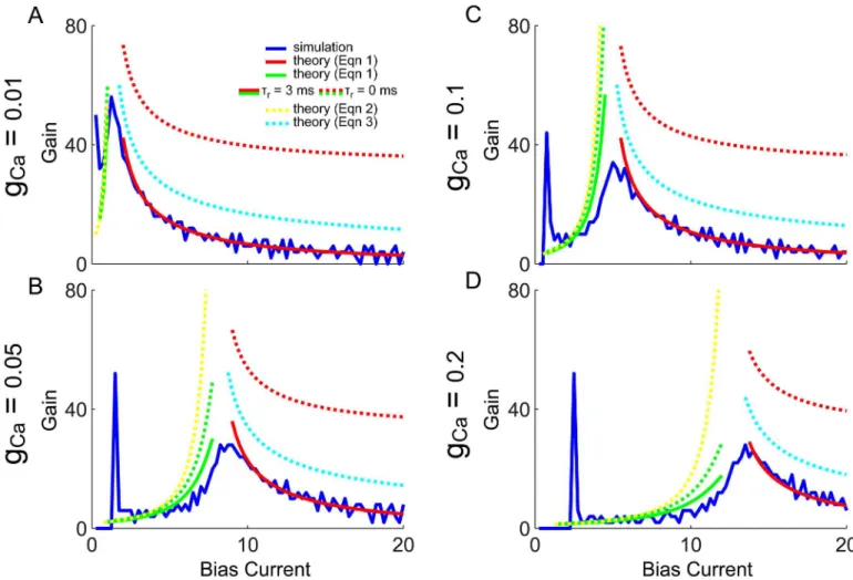
Eq (1)is plotted inFig 5, for bothτr= 3 ms (solid green and red) as well asτr= 0 ms (dashed green and red), superimposed with thefiring rate calculated by numerically simulating model

Eq (8)directly (black). The solid red dots indicateμwhich can be seen to clearly match the region where the slope of the f-I curves are greatest. Forμ>μthe solid red curves are in very good agreement with the black curve, and the saturation (or reduction in slope) can be seen to

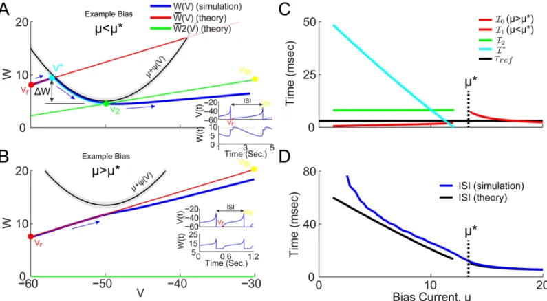
Fig 4. WV phase space projection of trajectories at low and high gainμvalues, for QIF withXr= 0.1 andCr=C1(Vr,Xr)(seeFig 3E) (A) Example

phase space trajectory at bias current,μ<μ*, forgCa= 0.2.Simulated trajectory projected into VW phase space (blue) has blue arrows indicating direction of motion in time. The theoretically predicted trajectory starts at the reset voltage,Vreset(red dot), and travels alongWðVÞ(red line) until it intersects

μ+ψ(V*) (black line) atV*(cyan dot). The grey band indicates the region ofj_V_

j< . At this point, thexandCvariable are free to decay (cyan curve) untilW reachesV2. ThenxandCare againfixed and give rise to a new mean adaptation currentW_{ðVÞ(seeEq (26), green line) connecting the pointV}

2(green dot) and the threshold voltage (yellow dot). Furthermore, the change inWbetweenV*andV2is assumed to beDW¼_W

ðV_{Þ ðmÞas indicated (and}

assumed byEq (23)). Insets showV(t) andW(t) as time series. (B) Example trajectory at bias current,μ>μ*, forgCa= 0.2. NowWðVÞ(red line) does not intersectμ+ψ(V), and directly connectsVr(red dot) andVth(yellow dot). (C) The time intervals for the different trajectory components are plotted as a function of bias current (forgCa= 0.2), using colors that match the trajectory components color in (A) and (B). The vertical dashed line indicatesμ*. (D) The sum of all the predicted intervals shown in (C) results in the predicted ISI (black), and the average ISI of the simulated data (blue) show how the total interval is dominated byIwhenμ<μ*.

doi:10.1371/journal.pone.0159300.g004

be due primarily to the refractory period,τr(compare solid and dashed red).μ<μthe solid green curves are in reasonable agreement with the black curves (considering the additional approximations needed) at least exhibiting the boosting nonlinearity effect, which does not change significantly withτr.

The gain, or slope of the f-I curves, can next be calculated by simply differentiatingEq (1)

with respect to bias current,G(μ) =@R(μ)/@μ, which is plotted inFig 6(green and red solid and dashed curves) for comparison with that calculated from the simulated f-I curves (blue). To derive a more intuitive approximate equation for the gain, the refractory period can be set to zero,τr= 0:

Gðm_Þ 1

ð I1

|{z} 0

þIþ I2

|{z} 2p

Þ2

@I

@m

jBj

½m ð2_pBAÞ2

jBj

ðmm_Þ2 ; for m<m

ð2Þ

GþðmÞ ¼

1

I2 0

@I0

@m

₂1

p

ffiffiffiffi

g2

m

r

¼

ffiffiffiffiffiffiffiffiffiffiffiffiffi

g2=4p 2

p

½m ðW0þW_mðV2W_mÞÞ

1=2 ; for m>m

_:

ð3Þ

Fig 5. Steady state firing rate, simulations and theory: QIF withXreset= 0.1 andCreset=C1(Vreset, Xreset).The firing rate is plotted for the numerical simulations in black, with analyticEq (1)in green and red, with solid forτr= 3 ms, and dashed forτr= 0 ms.

Forμ<μ, the change in ISI is dominated by the change inI(the segment fromVtoV2),

andI1andI2are roughly constant by comparison (seeFig 4C). This allowsG−to be reduced

toEq (2b), which diverges asμ!2πB−A. AlthoughAandBdepend onμ, plugging in

numer-ical values reveals that 2πB−A!μasμ!μ. Forμ>μthe gain depends only onI0and is found to scale as1₌pffiffiffi_{mfrom above, similarly to results for the simple QIF model [14], with a}

rescaled_{m. In this case the gain diverges whenm!}0_{which occurs whenμ=W0+Wm(V2−}

Wm)’μ, which is also very close toμ. This shows that the gain scales as 1/(μ−μ)2from

bel-low and as 1/(μ−μ)1/2from above, and explains why the peak gain should be nearμ=μ.

Eqs (2) and (3) are also superimposed inFig 6, where the dashed yellow and cyan curves are approximations to the dashed green and red curves, and the solid green and red curves are approximations to the blue curve. The dashed yellow and green curves are in reasonable close agreement, and the solid green does capture the main effect of the boosting nonlinearity (i.e. increase in gain with increasingμ), however ignoring the initial spike in gain at the onset of spiking (blue curves). The solid red curves match the blue curves even better than the green curves (as there were fewer approximations needed). Although the dashed red and cyan curves

Fig 6. f-I curve gain, simulations and theory: QIF withXreset= 0.1 andCreset=C1(Vreset,Xreset).The gain (or f-I curve slope) is plotted for the

numerically simulated model in blue, with the derivative ofEq (1)in green and red (solid and dashed). Additionally the approximate gain Eqs (2) and (3) are superimposed in yellow and cyan dashed lines. The peak of the blue gain curve occurs atμ*(vertical black line) where the theoretical predictions all diverge. Panels A-D correspond to increasing values ofgCa.

doi:10.1371/journal.pone.0159300.g006

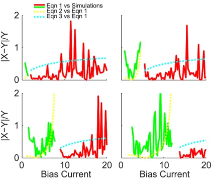
do differ significantly, it is a roughly constant amount and the cyan curve still captures the essential scaling features. To quantify the quality of these approximations, the absolute differ-ences of each pair, normalized by the target curve, is plotted inFig 7. Red and green compare

Eq (1)with the simulations, and yellow and cyan compare Eqs (2) and (3) with the derivative ofEq (1).

Theoretical firing rate for the QIF model with spike generated resets:

convergent iterative predictions

Coming back to the more physiological QIF model with spike generated reset conditions, which reproduces closely the HH model’s boosting nonlinearity as well as its bifurcations through bursting, the reset values,xresetandCreset, are no longer given. These reset values may be estimated via an iterative algorithm (seeModels and Methods), which may converge to a stable sequence of reset values. In the high bias region where the slow gating variable approxi-mation is valid, a self-consistency condition can be used to generate successive gating variable reset values (and in turn ISIs) similarly to that of Richardson [15]. As described inModels and Methods, becauseF(V)>0 in this regime, a result of the Fokker-Plank equation can be used to give the probability distribution of the voltage,p(V), which can be used to calculatexreset=hxi andCreset=hCi[15] according to Eqs (28)–(30). For low bias values where the slow gating vari-able approximation is not valid, however,Eq (30)no longer holds and the artificial action potential must be used to calculate new reset values.

Letting the algorithm iterate, it may converge to a sequence of identical ISIs (i.e. stable 1-spk limit cycle), a sequence of 2 or more ISIs which repeats (i.e. stable 2- or 3-spk limit cycle;

Fig 7. Comparison between results from the full theoretical and approximate gain equations.The quality of the full theoretical model is assessed by plotting the absolute difference between the derivative of

Eq (1)and the numerical simulations, normalized by the simulated gain, plotted in green and red forμ<μ*

andμ>μ*respectively. Additionally, the approximate gain Eqs (2) and (3) are compared to the derivative of

Eq (1)withτr= 0, plotted in yellow and cyan dashed curves.

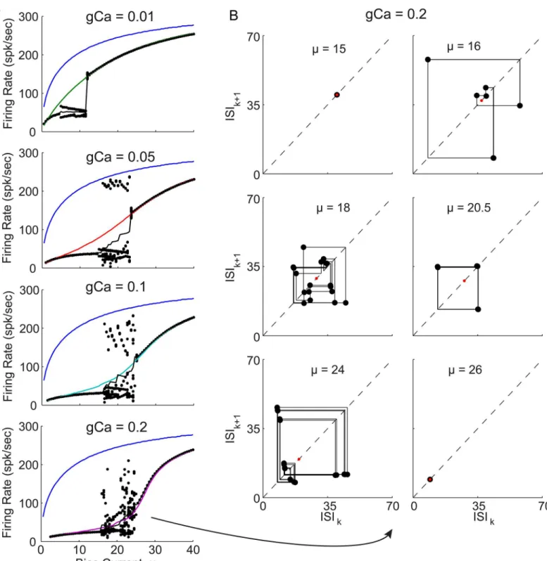
bursting), or even a sequence of ISIs that has no repeating patterns. After 20 iterations of tran-sient ISIs, convergence has generally been reached and the mean and standard deviation of the subsequent sequences of 1/ISIs was used to estimates the f-I curves, as plotted inFig 8A. The iterative theory can be seen to converge to stable 1-spk limit cycles in the limits of low and high bias current, as well as produce variable ISI sequences (red dashed) near the bursting in the QIF model (black dashed). The best agreement is actually achieved for the highest value ofgCa = 0.2 in the bottom right panel ofFig 8A, where two example bias currents are indicated by yel-low dots, which will be considered in the VW phase space beyel-low.

For the stable 1-spike limit cycles in reasonable agreement with the QIF simulations, the low and high bias example trajectories are plotted in the VW phase space inFig 8B and 8C. These two trajectories can be seen to have the same fundamental geometry of those inFig 4: in the high bias region the trajectories do not encounter the parabola,μ+ψ, while for low bias currents, they do. However, inFig 8Bthe simulated QIF trajectory (blue curve) crosses the black parabola and changes direction in V, before crossing the parabola again and crossing back over itself (which is only possible since this is really a 3D phase space projected into 2D) before increasing to threshold. It is this trajectory that result in the specific AHP shape in which the voltage changes directions twice. In this caseEq (22)must be used to estimate the calcium decay fromVtoV2, which is compared to that calculated analytically viaEq (21)in

theFig 8Binset (seeModels and Methodsfor details). Once the time interval for each separate component is calculated as described inModels and Methods, the voltage distribution during each segment can be estimated and in the bottom of 8B can be seen to provide a not very accu-rate match to the simulation (compare black and blue curves), but it does have the marked fea-tures of the combined red and cyan peaks. These distributions in 8B, however, are not used in the iterative algorithm. For example 2 in the high bias regime (Fig 8C), bothVandWcan be seen to increase monotonically from reset to threshold, and the resulting voltage distribution is in much better agreement with the simulations.

Although the iterative theory captures the essential phase space geometry to explain the boosting nonlinearity, the results in the regions of bursting are considered next. InFig 9(left) the FI curves of the QIF with spike are again plotted, but now with each 1/ISI in the sequences (black dots). Clearly these do not follow the ordered period adding bifurcations see in Figs1E

and2E. Although there does appear to be a window of order with a stable 3-spike burst (seeFig 9right), this 3-spike sequence does not have the same structure as the bursts in Figs1and2

(i.e. short-short-long ISI sequences) and may instead be considered an alternation of 1-spk and 2-spk bursts. While the iterative theoretical predictions do capture the low to high gain transi-tion across the boosting nonlinearity, they do fail entirely at capturing the period adding bifur-cations through bursting.

Conclusions

To summarize, in this paper it was shown that a conductance-based Hodgkin-Huxley type ves-tibular neuron model with high voltage-activated calcium and calcium-activated potassium currents, can exhibit a boosting nonlinearity for increased calcium conductance,gCa. In addi-tion, the model exhibits a period adding bifurcation through bursting for intermediate bias cur-rents separating the low and high gain regions of the boosting nonlinearity, with an AHP in the low gain region. In order to isolate the mechanism underlying the boosting nonlinearity, the HH model was reduced to a generalized QIF model that preserves the subthreshold bifurcation structure. With an artificial action potential to activate the gating variables, the QIF model reproduces the boosting nonlinearity and the bifurcation through bursting and AHP. To fur-ther simplify the model and tease apart the necessary ingredients for a boosting nonlinearity,

QIF models were created that use fixed values for,ΔxandΔC, and finally for,xresetandCreset. For this simplified QIF a slow gating variable approximation was used as a starting point to derive an analytic equation for the f-I curves, and approximate expressions for the gain (i.e. its slope), showing the gain to be peaked atμ=μ. An intuitive geometrical picture of how the tra-jectories through VW phase space shows that they differ qualitatively in the low and high bias regions of the boosting nonlinearity, and that these two types of trajectories provide the basis for understanding the boosting nonlinearity and deriving an expression forμ. Finally, in the case of spike generated reset conditions, it is shown that an iterative algorithm can find stable 1-spk limit cycles that provide reasonable agreement in the limit thatμ!0, and excellent agreement in the high bias regime.

Comparison to other two- and three-variable adaptive models

Previously a two-variable adaptive QIF model was studied and found to exhibit a similar boost-ing nonlinearity [14]. This model used a fixed reset value for its adaptation current,W, such that it would be resetabovethe parabolic functionμ+ψ(V) for low bias, causing the voltage to initially move in the negative direction until it can cross belowψand begin moving positively, towards threshold. Onceμis increased such that it is greater thanWreset, the trajectories are then reset belowψand increase monotonically towards threshold. This is a very similar mecha-nism of boosting, whereby spiking trajectories in the low gain region must cross (or come very close to) the V-nullcline,W_{=ψ(V), while trajectories in the high gain region do not. This} mechanism also results in an AHP in the low gain region, where the voltage initially decreases through a slow minimum, but only changing directions once. However, because phase space trajectories can not cross over themselves, the low gain region only emerges when the reset conditions start the trajectory aboveψ. In the three-variable adaptive QIF model considered here, the projections in the VW plane can cross themselves only because they have an extra dimension due to thexandCvariables, andW(x,C). This allows trajectories in the QIF model to start below the V-nullcline, cross up above it, loop back below, cross themselves and off towards threshold. This is what gives my 3-variable QIF model’s spikes their signature AHP shape which initially increases before decreasing, unlike two-variable models.

Although the two-variable QIF model of Shlizerman and Holmes does not burst [14], its close relative the adaptive exponential-IF (aEIF, also two-variable) can produce bursting [11,12], when the adaptation variable reset condition is insteadWreset=W(tspk) +ΔW. This produces bursting in a similar way as the adaptive QIF model: multiple short ISIs occur (which do not intersectψ) withWincreasing each time, untilWhas accumulated enough that the trajectory does intersectψand a long ISI occurs, terminating the burst. Although the exponential function in the aEIF model changes the shape ofψ, it does not change the basic concave-up geometry cap-tured by the QIF. As such, it may be expected that the regions of such aEIF models that produce

Fig 8. WV phase space projection for QIF model with spike waveform, and convergent iterative theoretical predictions forμ>μ*andμ!0.

(A) Firing rate for QIF with spike waveform, as inFig 3A, in solid black lines forgCa>0 (as indicated), and blue curves forgCa= 0. Iteratively estimated theoretical predictions (seeModels and Methodsfor details) are superimposed in red, with solid lines indicating the mean 1/ISI, and dashed lines indicating standard deviation (SD) of 1/ISIs (the bursting patterns will be considered in the next figure). Theory shows excellent agreement above the bursting region whereF(V)>0, and reasonable agreement at very low bias currents. Two example bias currents are indicated by numbered yellow circles in the bottom right panel. (B) Low bias example trajectory in VW phase space. Simulated trajectory in blue (with direction of flow indicated by blue arrows), with theoretical trajectory connectingVresettoV*(red line), thenV*toV2(cyan line), and finallyV2toVth(green line). Inset shows the cyan trajectory in terms of decaying variablesx*(t) andC*(t), and howEq (22)captures the initial increase and then decrease in the calcium concentration, whileEq (21)does not. Below, the corresponding voltage probability density for the simulated trajectory (blue), and each of the red, cyan, and green segments (independently normalized), as well as their weighted combination (black, seeModels and Methods). (C) Same as panel B, but for the high bias example point.

doi:10.1371/journal.pone.0159300.g008

Fig 9. Iterative theoretical predictions for QIF model with spike waveform: stable and unstable 1-spike limit cycles.(A) f-I curves for QIF model with spike waveform, each panel comparinggCa= 0 (blue) withgCa>0 as indicated (color), as well as the theoretical predictions (black). The iterative theory produces a sequence of ISIs, the final 20 are plotted as 1/ISI at each bias (black dots), and their average value versus bias is superimposed (solid black). (B) For the highestgCavalue, ISI return maps are shown for six illustrative bias current values starting with a low bias stable 1-spk limit cycle (top left panel), through bifurcations to aperiodic spiking, with windows of repeating sequences, and back to stable 1-spk limit cycles at high biases (bottom right panel). The same 20 ISIs from A are also plotted in B. It can be seen that atμ= 20.5, a stable sequence of 3 intervals repeats. Similarly, the bottom left panel

shows similar sequence of 3 ISIs almost repeats, but 2+ slightly different versions of it repeat, illustrating how regions with stable N-spike ISI sequences transition to other regions with stable M-spike ISI sequences.

bursts might also indicate the presence of a boosting nonlinearity, however this has not been reported [11,12]. In addition, although the aEIF model generally uses a simpler linear equation for the dynamics of the adaptation variable such asW_ ¼ ½aðVVwÞ W=tw, it still requires

the further simplification thata= 0, to compute thathWi=ΔWa priori and apply a slow gating variable assumption for an analytic solution [10,16].

Finally, Richardson analyzes a three-variable adaptive model very similar to ours [15], with spike-triggered calcium and calcium activated potassium, however he uses an artificial action potential withVmax= 0, that decays linearly to the resetVreset. He also avoids the problem of not knowing the value ofhWiby using the slow gating variable assumption and self-consis-tency criterion to find it iteratively. He does not report a boosting nonlinearity or bursting, but remains in a region of parameter space whereF(V)>0 and no AHP [15]. In addition, different spike shapes with the QIF did have a significant effect on whether or not the adaptation cur-rents were strong enough to produce either boosting or bursting, which is one possible expla-nation for our differing results. However, different values for the conductancesgCaandgKCa are used as well. Although the goal of this study was to understand the mechanisms that pro-duce boosting in the HH model, the ultimate goal is to relate it back to experimental data from the vestibular system, and how it might be functionally relevant.

Correspondence to vestibular nuclei neuron data

The HH model used in this paper is already a simplified version of the original vestibular nuclei neuron model developed by Av-Ron et al. [5], where only the ion channels necessary to gener-ate the boosting nonlinearity were included. These channels were originally tuned to produce the characteristic bi-directional AHP that goes up and then down before rising to threshold (switching direction twice). This very AHP appears to be a signature that the model would likely produce a boosting nonlinearity (and bursting) if driven to sufficiently high bias currents that the AHP no longer occurs. However, this model was originally developed forin vitro prep-arations where the average baseline firing rate is much lower (i.e.*30–50spk/s) than in alert behaving animals (i.e.*60–80spk/s) [6]. This may be why such a boosting nonlinearity has not yet been observedin vitro. One would expect that if thein vitrorecordings used current injections large enough that the AHP could no longer occur, that this would also be sufficiently large to reveal a boosting nonlinearity as well, an experimentally testable prediction of this manuscript.

It is also important that neurons are considerably more variablein vivo, requiring an addi-tive noise term in the model [6]. Including such increased noise, simulations of the HH model still show the boosting nonlinearity, while the noise is sufficient to disrupt the bursting (not shown). Furthermore, analysis of the data in Massot et al. [4] has shown no evidence of burst-ingin vivo. To further improve the correspondence between the HH model and VN neurons, additive noise could be added to provide the appropriate coefficient-of-variation of the sponta-neous spiking activity [4]. However, it is known that different noise intensities may be needed during spontaneous and driven stimulation conditions, as was found for vestibular afferent models [17]. Experimental efforts should therefore be made to measure both the mean firing rate and its variance as functions of bias current, using different stimuli, to further constrain accurate VN neuron models.

Implications for sensory information processing in the vestibular system

The boosting nonlinearity was originally found in vestibular-only (VO) neurons in VN using narrow band noise stimuli with low (0–5 Hz) and/or high (15–20 Hz) frequency content, and it was found that when presented together the high frequency stimuli masked the response to

low frequency stimuli [4]. A linear-nonlinear (LN) cascade model of the data could explain this masking effect and predict the % attenuation for additional stimuli. The statistics of naturally occurring head movements in primates have since been recorded [18] and indeed been found to have significantly higher power over the low frequency range than the high frequency range, making it unclear whether such masking would occur under natural conditions. This could be explored in a model using stimuli with naturalistic frequency content combined with afferent filters. Additionally, natural stimuli have combinations of angular and linear movements, which could also lead to masking between different axes of motion, rather than different fre-quency bands within one axis of motion.

It is well known that when neurons are driven across a common rectifying nonlinearity, it can result in increased spiking precision, with information lost about the stimuli in the zero gain region of the nonlinearity which also has a firing rate of zero. It is therefore possible that the boosting nonlinearity could allow the same increased spiking precision, potentially indica-tive of temporal encoding, to coexist with a standard rate coding since the low gain region still has non-zero gain and firing rate. Further studies with this model could therefore investigate the possibility of simultaneous rate and temporal coding, under natural stimulus conditions. Finally, it should be pointed out that VO neurons are known to respond robustly to pas-sively applied stimuli (i.e. head movements externally generated by the experimenter), but to show*70% to the self-generated stimuli studied [19], and that the large majority of natural stimuli recorded by Schneider et al. was indeed self-generated [18]. This suggests a potential role for the boosting nonlinearity: if self-generated stimuli elicit responses that are not suffi-ciently attenuated and cross the boosting nonlinearity, an increased level of spiking precision (or population synchrony) could signal a potential problem, without entirely disrupting the lin-early decodable information remaining about the stimulus in the firing rate.

Models and Methods

Full HH model

The Hodgkin-Huxley (HH) type model of a VN neuron developed by Av-Ron et al. [5] and adapted by Schneider et al. [6] is studied in this paper. Specifically, the model includes spiking sodium and potassium currents governed by the single activation variable,n(as in the Morris-Lecar model), as well as a voltage-activated calcium current and calcium-activated potassium current, each governed by the activation variables,xandC, respectively. The additional cal-cium current, is activated by high voltages that occur during an action potential, and serves pri-marily to let calcium into the cell with only a small effect on membrane voltage. The additional potassium current, however, is only activated by the calcium that enters the cell when it spikes, and serves to reduce the voltage and prevent spiking. The additional persistent sodium and hyperpolarization-activated currents present in [5,6] have been removed, as they are not nec-essary for the model to generate the boosting nonlinearity being investigated. This results in a 4-dimensional spiking neuron model governed by the following differential equations:

Cm

dV

dt ¼ H1ðV;n;x;CÞ ¼mI_ionsðV;n;x;CÞ

dn

dt ¼ H2ðV;nÞ ¼ ½n₁ðVÞ n=t_n

dx

dt ¼ H3ðV;xÞ ¼ ½x₁ðVÞ x=t_x

dC

dt ¼ H4ðV;x;CÞ ¼ ½C₁ðV;xÞ C=tC:

Iions=INa+IK+Ileak+ICa+IKCa, withC1¼ KRICa, and the currents are given by the

follow-ing additional equations:

INaðV;nÞ ¼ gNam

3

1ð1nÞðVVNaÞ

IKðV;nÞ ¼ gKn

4

ðVVKÞ

IleakðVÞ ¼ gLðVVLÞ

ICaðV;xÞ ¼ gCax

2

ðVVCaÞ

IKCaðV;CÞ ¼ gKCa

C CþKd

ðVVKÞ;

ð5Þ

where the steady state activation variables obey the following equation:

z₁ðVÞ ¼1_=½1_þexp½2_aðzÞ_ðVVðzÞ

1=2Þ, forz2{n,x}. All parameters are as used by Schnei-der et al. [6], unless otherwise stated. The calcium current equationICahas also been modified from Schneider et al. to remove the calcium saturation term, Kr

CþKr, to further simplify the model while preserving the boosting nonlinearity.

The fixed points (FPs) of the HH model can be found by setting the equationsH1=H2=H3

=H4= 0, then solving for,n=n1(V),x=x1(V),C=C1(V), whileVmust be found by

plugging these intoH1, and numerically finding the zeros of

H1ðV;n;x;CÞ ¼ mg_LðVV_LÞ g_Nam 3

1ðVÞð1nðVÞÞðVVNaÞ

gKn

4

ðVÞðVVKÞ

gCax

2

ðVÞðVVCaÞ gKCa

C_ðVÞ

KdþCðVÞ

ðVVKÞ;

ð6Þ

for a range of bias current values,μ. The stability of thefixed points can then be found by look-ing at the eigenvalues of the followlook-ing matrix

L_HH ¼

@H1=@V @H1=@n @H1=@x @H1=@C

@H2=@V @H2=@n 0 0

@H3=@V 0 @H3=@x 0

@H4=@V 0 @H4=@x @H4=@C

0 B B B B B B B @ 1 C C C C C C C A

; ð7Þ

where the FP is stable if all its eigenvalues have negative real parts.

SettinggCa= 0 (and in turnC= 0), it is well known thatH1(V) has a cubic form (or sideways

‘S’shape), with a local minimum at a lower voltage and a local maximum at higher voltage. This shape does not change, but is translated vertically with changes in the bias current,μ. For sufficiently low values ofμthere are three fixed points, only that with the lowest voltage is sta-ble, and corresponds to the steady state resting potential. Asμis increased, the two fixed points at lower voltages annihilate in a saddle-node bifurcation at which point there is no stable fixed point, and the model generates action potentials via a stable limit cycle. It is also possible (whengCa>0) for the lowest voltage fixed point to lose stability via a Hopf bifurcation. In this case the spiking limit cycle can coexist with all three unstable fixed points, with the two lower voltage fixed points annihilating at yet higher values ofμ.

Simplified QIF model

In order to find an analytic equation explaining the change in gain of the boosting nonlinearity, a reduced integrate-and-fire (IF) type model is used, that preserves the FP bifurcation structure of

the HH model. This is done by removing the gating variable,n, and replacing the currents,IL(V) +INa(V) +IK(V), with a nonlinear functionψ(V), and a voltage threshold and reset. Although simple constant or linear functions can be used forψ(V), a concave up function is needed to reproduce the second bifurcation of two subthreshold fixed points in the case of the Hopf bifur-cation at spiking onset. The simplest of these functions is the quadratic,ψ(V) =g2(V−V2)2,

resulting in the generalized QIF model, governed by 3 differential equations:

C_mdV

dt ¼ F1ðV;x;CÞ ¼mþcðVÞ I_CaðV;xÞ I_KCaðV;CÞ

dx

dt ¼ F2ðV;xÞ ¼ ½x₁ðVÞ x=t_x

dC

dt ¼ F3ðV;x;CÞ ¼ ½C₁ðV;xÞ C=t_C;

ð8Þ

where the only new parameters to define areg2andV2.

In addition, the QIF model requires a boundary condition such that when the voltage reaches a threshold,Vth, a spike is said to have occurred, and the voltage is returned to a reset value,Vreset, for an absolute refractory period,τr. However, because the high voltages occurring during the action potential are needed to drive the voltage-activated calcium currents, a simple piece-wise linear function,Vspk(t), is used during the refractory periodtspk<t<τr(similar to Richardson [15]). The spike shape rises linearly to a maximum, and then decays linearly to the reset voltage according to

VspkðtÞ ¼ Vthþ

VmaxVth

t1

t; : : : : : : for 0_t<t

1

Vmaxþ

VrVmax

t_rt1

ðtt1Þ; : :for t1t<t_r

ð9Þ

wheret= 0 corresponds to the spike times. In this paper, the spike shape parameters,Vmax= 30 mV,t1= 0.4 ms, andτr= 3 ms are used. This results in thexandCgating variables changing according tox(tspk)!x(τr) =x(tspk) +Δx, andC(tspk)!C(τr) =C(tspk) +ΔC, whereΔxandΔC are calculated by pluggingEq (9)intoEq (8b) and (8c)and numerically integratingx(t) andC

(t) fromtspktoτref.

The QIF model can be further simplified by removingVspk(t) and using either fixedΔxand

ΔC, or fixedxresetandCreset, resulting inx(tspk+τr) =xresetandC(tspk+τr) =Creset. This results in two more parameters, eitherxresetandCreset, orΔxandΔC, which must be defined, instead ofVmaxandt1.

The fixed points (FPs) of this simplified QIF model do not depend on the artificial spike shape or reset boundary conditions, and can be found by setting the equationsF1=F2=F3= 0,

and solving for,x=x1(V),C=C1(V), as before, withVnow being found by plugging

these intoF1, and numerically finding the zeros of

F1ðV;x;CÞ ¼ mg2ðVV2Þ g_Cax 2

ðVÞðVVCaÞ gKCa

C_ðVÞ

KdþCðVÞ

ðVVKÞ

¼ 0_:

ð10Þ

matrix

LQIF¼

@F1=@V @F1=@x @F1=@C

@F2=@V @F2=@x 0

@F3=@V @F3=@x @F3=@C

0 B B B @ 1 C C C A

: ð11Þ

Although the subthresholdfixed points and their stability depend only on the system ofEq (8), the reset values,xresetandCreset, behave as additional bifurcation parameters, similarly to the reset parameters in the adaptive two-variable models studied by Naud et al. [12].

To estimate the QIF model parametersg2andV2from the HH model,gCacan be set to zero, and the nonlinear functions inH1(V,n) expanded to second order inV, around its

approxi-mate minimum (−50 mV, seen by plotting),

H1ðVÞ ¼ mg_LðVV_LÞ g_Na m 3

1ðVÞ |fflfflffl{zfflfflffl} a1þb1ðVþ50_Þ

ð1 _n

1ðVÞ |fflfflffl{zfflfflffl} a2þb2ðVþ50_Þ

ÞðVVNaÞ

gK n

4

1ðVÞ |fflfflffl{zfflfflffl} a3þb3ðVþ50_Þ

ðVVKÞ;

mþkþaðVhÞ2

;

ð12Þ

witha1 ¼m 3

1ðV¼ 50Þ,a2=n1(V=−50),a3 ¼n 4

1ðV¼ 50Þ,b1 ¼@m 3

1=@VðV¼ 50Þ,

a2=@n1/@V(V=−50), anda3 ¼@n 4

1=@VðV ¼ 50Þ. Solving for a and h can then be used to

estimateg2andV2, however, the valuesg2= 0.1 andV2=−50 mV do a sufficient job to

repro-duce the HH model’s features of interest.

A complete solution of this model would result inV(t),x(t), andC(t), and can result in tonic firing of a single repeated interspike-interval (ISI), or bursts of two or more ISIs in a sequence which repeats, as well as possibly aperiodic spiking with sequences of ISIs which never repeat. In the entire 3D phase space, there is a single trajectory deterministically connectingVrtoVth, for each possible combination ofxresetandCresetvalues which occur at the voltage reset. The trajectories cannot intersect and the entire phase space of trajectories is defined by the system ofEq (8), but the particular trajectory for each ISI is determined by the values ofVreset,xreset, andCreset. ThexandCvalues occurring at the voltage threshold may of course be different, and not necessarily result in the same reset values, and may therefore be reset onto a different nearby trajectory in phase space. In my simplified QIF with fixedxresetandCresetreset values, together withVreset, the voltage is reset onto the same trajectory after each spike, resulting in only tonic spiking of a single repeated ISI. In this case the ISI can be estimated analytically, with the values ofxresetandCresetdefined as model parameters.

Slow gating variable approximation for fixed reset conditions

The additional gating variables,xandC, have time constants of 10 and 20 ms, compared to the average membrane time constant of2 ms, and can thus be assumed to vary slowly by com-parison (i.e._x_ _C_ _V__{). Although the gating variables may be reset instantaneously during}

the refractory period following spiking, this approximation only needs hold from the end of the refractory period until the next spike. Additionally subthreshold regions in which this approximation breaks down, such as during an AHP, will be identified and dealt with sepa-rately. This assumption allows the gating variables to be approximated by their initial values,x

xresetandCCreset. As a result, the additional calcium related currents depend only onV,

and can be defined in the adaptation current,WðVÞ, as

WðVÞ ¼ ICaðV;xrÞ þIKCaðV;CrÞ

WðVÞ ¼ gCax

2

r þgKCa

Cr

CrþKd

|fflfflfflfflfflfflfflfflfflfflfflfflfflfflfflfflfflfflffl{zfflfflfflfflfflfflfflfflfflfflfflfflfflfflfflfflfflfflffl} Wm

V gCax

2

rVCaþgKCa

Cr

CrþKd

VK

|fflfflfflfflfflfflfflfflfflfflfflfflfflfflfflfflfflfflfflfflfflfflfflfflfflfflffl{zfflfflfflfflfflfflfflfflfflfflfflfflfflfflfflfflfflfflfflfflfflfflfflfflfflfflffl} W0

WðVÞ ¼ W0þW_mV:

ð13Þ

WðVÞis simply linear inV, always having a positive slope (except whengCa= 0, causingW0=

Wm= 0). This results in the system of Eqs in 8, reducing to a single differential equation

dV

dt ¼FðVÞ ¼mþcðVÞ

WðVÞ; ð14Þ

whereψ(V)>0 represents the spike-generating currents which always drive the membrane voltagetowardsthreshold, andWðVÞ>0_{represents the calcium and calcium-activated}

potas-sium currents which always act to drive the voltageawayfrom threshold. It is becauseVK<Vr VVth<VCa, that although the calcium current always serves to depolarize the membrane, the stronger calcium-activated potassium current always serves to hyperpolarize the cell.

In the approximate 1D system defined byEq (14),μ+ψ(V) is a parabola with its minimum atμ, andWðVÞis a line with positive slope, independent ofμ. This gives two possible scenarios: for low enoughμthe parabola and line intersect, while for high enoughμthe parabola and the line do not intersect. If there is an intersection, thenF(V) = 0 at that voltage, and the approxi-mate 1D system should have afixed point, but since the system is really a 3D system, it only indicates that the slow gating variable approximation breaks down. Although the initial condi-tions at voltage reset could correspond to a region where_{W >c, as in [12,14], this does not}

occur for the model parameters considered in this paper.

Since the parabola is translated linearly withμ, there must always exist a bias current,μ, such thatF(V)> forμ>μ, where the parabola,μ+ψ−and the line,W intersect at a single

point. The value ofis chosen to be 0.5, small but non-zero, to avoid divergent calculations involving 1/F(V). ForgCa>0, the bias currentμ, can be defined byF(μ,V) =:

m_¼ð2g2V2þW_mÞ 2

4_g

2

g2V

2

2 þW0þ: ð15Þ

Forμ>μ,F(V)> and it is straightforward to integrateEq (14)from reset to threshold to calculate the ISI (consider this case 1). But forμ<μ,V_ < for a range ofVin which the slow gating variable assumption cannot be made andEq (14)cannot be used (consider this case 2). It should be noted that in the limit thatgCa!0,μ!μ, as expected.

Case 1_:μ>μand_jV__{j> Withμ>μandjV}__{j> , the voltage moves monotonically}

from reset to threshold, andEq (14)can be integrated to get the time interval

I0ðmÞ ¼

Z Vth

Vr

dV

FðVÞ: ð16Þ

PluggingEq (14)into 16 results in

I0 ¼

Z Vth

Vr

dV

mþg2ðV

V2Þ 2

¼ ffiffiffiffiffiffiffi1

g2m

p tan1

ffiffiffiffiffiffiffi

g2m p

ðVthVrÞ

mþg2ðV_th

V2ÞðV_r

V2Þ

;

where the new variables:_m¼mW

0W_mðV2W_mÞ,

V2 ¼V2þW_m=2g2have been defined. In the limit thatgCa!0,m!mandV2!V2, and the solution to the to the simple QIF model is recovered [14]. Further lettingg2!0, the well known IF model ISI,

IIF¼ ðVthVrÞ=m, results. Case 2_:μ<μ

Case 2a_:VrVV,with_V_ _{> For low bias currents,}

μ<μ, there are two voltages at which the depolarizing current,μ+ψ(V) is balanced by the hyperpolarizing adaptation cur-rent,WðVÞ, corresponding tofixed points whereF(V) = 0. However, at the reset point, (Vr,

Wr),F(V) is positive and remains so until the voltage reaches the-neighbourhood of the lower intersection point,V_{, defined by}

V_¼ 2_g

2V2þW_m

ffiffiffiffiffiffiffiffiffiffiffiffiffiffiffiffiffiffiffiffiffiffiffiffiffiffiffiffiffiffiffiffiffiffiffiffiffiffiffiffiffiffiffiffiffiffiffiffiffiffiffiffiffiffiffiffiffiffiffiffiffiffiffiffiffiffiffiffiffiffiffiffiffiffiffiffiffiffiffiffiffiffiffi

ð2_g

2V2þW_mÞ 2

4_g

2ðmþg2V 2 2 W0Þ

q

2_g

2

; ð18Þ

whereF(V) =. In this case, the voltage evolves according toEq (14)fromVrup toV, with

m<0_{in this region, resulting in}

I1 ¼

Z V

Vr

dV

j_{mj þg}

2ðV

V2Þ 2

¼ 1

2 ffiffiffiffiffiffiffiffiffiffi_g

2jmj

p ln

½1_þ ffiffiffiffiffiffiffiffiffiffiffiffi_g

2=jmj

p

ðV

V2Þ½1

ffiffiffiffiffiffiffiffiffiffiffiffi

g2=jmj

p

ðVr

V2Þ ½1 ffiffiffiffiffiffiffiffiffiffiffiffi_g

2=jmj

p

ðV

V2Þ½1þ

ffiffiffiffiffiffiffiffiffiffiffiffi

g2=jmj

p

ðVrV2Þ

;

ð19Þ

with_mandV

2defined as inEq (17).

Case 2b_:VVV

2,withjV_j< Once the membrane voltage has reachedV,F(V)

and the slow gating variable approximation can no longer be made, andxandCmust be allowed to evolve in time. It is assumed that atV_{the gating variables result in an adaptation}

currentW_>

μ, and that they can now decay until the adaptation current,W(t), reaches the bottom of the parabola atμ−. In this region,V_ 0andV ðVþV2Þ=2

V_{, so that one}

can solveF2andF3forx(t) andC(t). Assumingx1x1ðVÞ,Eq (8b)gives

x_{ðtÞ ¼x}

1 ðx1xrÞet =t_x;

ð20Þ

by requiringx(t= 0) =xr. Now to solveEq (8c), one should plug inx(t), as calculated above, however to get an analytic solution, it is assumed thatx_{ðtÞ x}

1, andC1 C1ðV;x1Þis

defined, resulting in

C_{ðtÞ ¼C}

1 ðC1CrÞet

=tC: ð₂₁Þ

To get a more accurate prediction,Eq (8c)can be numerically integrated according to

C

2ðt_iÞ ¼C2ðt_i1Þ þDt½C₁ðV;xðt_i1ÞÞ C2ðt_i1Þ=t_C; ð22Þ

withC(t0) =Cr, in either case.

The gating variable dynamics in turn cause changes inW_{(t). It is then assumed thatW(t)} decays until it reaches the bottom of the parabolaμ+ψ(V)−, atV2. This time can then be

solved for,W_{(t) =μ}

−,

W_{ðtÞ ¼g}

CaxðtÞ

2

|fflfflffl{zfflfflffl} a1þb1t

ðV_V

CaÞ þgKCa

C_ðtÞ

C_{ðtÞ þK} d |fflfflfflfflfflfflffl{zfflfflfflfflfflfflffl}

a2þb2t

ðV_V

KÞ ¼m

ð23Þ

by expanding tofirst order in time. The resulting coefficients are:a1¼x 2

r,a2=Cr/(Kd+Cr),

and

b1 ¼

@x_ðtÞ2

@t t¼tx

¼2x

_ðt

xÞðx1xrÞ

t_x e

1

b2 ¼

@ @t

C_ðtÞ

KdþCðtÞ

t¼tC

¼ KdðC1 CrÞ

ðKdþCðtCÞÞ

2

t_Ce

1

:

ð24Þ

This allowstto be found,

I ¼ t0_¼m ½gCaa1ðV

_V

CaÞ þgKCaa2ðVV_KÞ

gCab1ðVVCaÞ þgKCab2ðVVKÞ

¼ m_BA;

ð25Þ

whereA[gCaa1(V−VCa) +gKCaa2(V−VK)] andBgCab1(V−VCa) +gKCab2(V− VK). This shows thatArepresents the amount of adaptation current,W, when the voltage enters theV_ < region atV_{, whileBrepresents rate of change of adaptation current, due to}

the decay of the gating variablesxandC. This gives the simple geometric interpretation that the time intervalIis equal to the“distance”thatWmust travel, divided by the“velocity”at whichWtravels.

At this point in time, the adaptation currentWhas decayed toW(t) =μ−, andV(t) = V2, and the voltage is once again free to increase monotonically until threshold.

Case 2c_:V2VVth,with_V_ _{> For the remaining trajectory, I require a new adaptation} current,W_{, using the decayed gating variables instead of their initial reset values. However, I}

also require that_WðV

2Þ ¼mto have the desired initial conditions, resulting in

W_{ðVÞ ¼ W}

0þW_mV

W

m ¼ gCaxðtÞ

2 þgKCa

C_ðtÞ

KdþCðtÞ

W

0 ¼ mW_mV2:

ð26Þ

Eq (14)can then be integrated fromV2toVth, resulting in

I2 ¼

Z Vth

V2

dV

m_þg

2ðV

V

2Þ 2

¼ ffiffiffiffiffiffiffiffiffi1

g2m

p tan1

ffiffiffiffiffiffiffiffiffi

g2m p

ðVthV2Þ

m_þg

2ðV_th

V

2ÞðV2

V

2Þ

;

ð27Þ

where the new variables:_{m ¼mW}

0 WmðV2W_mÞ,

V

2 ¼V2þW_m=2g2are again defined. Once the voltage has reached threshold, in this case thexandCvariables have decayed from their reset values to new values at the occurrence of the new spike,x(tspk) =x(t) andC (tspk) =C(t). In this case, thefixed gating variable reset conditions are independent of these threshold values, but in the case of the spike generated resets, they will depend strongly on these threshold values.

Iterative Theoretical Predictions: Stable and Unstable Limit Cycles