Estimating cloud optical thickness and associated surface UV irradiance from SEVIRI by implementing a semi-analytical cloud retrieval algorithm

(1)

ACPD

12, 691–721, 2012

Estimating cloud optical thickness

P. Pandey et al.

Title Page

Abstract Introduction

Conclusions References

Tables Figures

◭ ◮

Back Close

Full Screen / Esc

Printer-friendly Version Interactive Discussion

Discussion

P

a

per

|

Dis

cussion

P

a

per

|

Discussion

P

a

per

|

Discussio

n

P

a

per

|

Atmos. Chem. Phys. Discuss., 12, 691–721, 2012 www.atmos-chem-phys-discuss.net/12/691/2012/ doi:10.5194/acpd-12-691-2012

Atmospheric Chemistry and Physics Discussions

This discussion paper is/has been under review for the journal Atmospheric Chemistry and Physics (ACP). Please refer to the corresponding final paper in ACP if available.

Estimating cloud optical thickness and

associated surface UV irradiance from

SEVIRI by implementing a semi-analytical

cloud retrieval algorithm

P. Pandey1,2, K. De Ridder1, D. Gillotay3, and N. P. M. van Lipzig2

1

VITO – Flemish Institute for Technological Research, Mol, Belgium

2

Department of Earth- and Environmental Sciences, K.U. Leuven, Leuven, Belgium

3

Belgian Institute for Space Aeronomy, Brussels, Belgium

Received: 6 November 2011 – Accepted: 21 December 2011 – Published: 9 January 2012 Correspondence to: P. Pandey (praveen.pandey@vito.be)

(2)

ACPD

12, 691–721, 2012

P. Pandey et al.

Title Page

Tables Figures

◭ ◮

Back Close

Full Screen / Esc

Discussion

P

a

per

|

Dis

cussion

P

a

per

|

Discussion

P

a

per

|

Discussio

n

P

a

per

|

Abstract

In this paper, we describe the implementation of the Semi-Analytical Cloud Retrieval Algorithm (SACURA), to obtain scaled cloud optical thickness (SCOT) from satellite imagery acquired with the SEVIRI instrument and surface UV irradiance levels. In es-timation of SCOT particular care is given to the proper specification of the background

5

(i.e., cloud-free) spectral albedo and the retrieval of the cloud water phase from re-flectance ratios in SEVIRI’s 0.6 µm and 1.6 µm spectral bands. The SACURA scheme is then applied to daytime SEVIRI imagery over Europe, for the month of June 2006, at 15-min time increments. The resulting SCOT fields are compared with values obtained by the CloudSat experimental satellite mission, yielding a negligible bias, correlation

10

coeffi_{cients ranging from 0.51 to 0.78, and a root mean square di}ff_{erence of 1 to 2} SCOT increments. These findings compare favourably to results from similar intercom-parison exercises reported in the literature. Based on the retrieved SCOT from SEVIRI and radiative transfer modelling approach, simple parameterisations are proposed to estimate the surface UV-A and UV-B irradiance. The validation of the modelled UV-A

15

and UV-B irradiance against the measurements over two Belgian stations, Redu and Ostend, indicate good agreement with the high correlation, index of agreement and low bias. The SCOT fields estimated by implementing SACURA on imagery from geo-stationary satellite are reliable and its impact on surface UV irradiance levels is well produced.

20

1 Introduction

Clouds play an important role in the Earth’s climate system. In addition to Earth’s hydro-logical cycle (Lin et al., 2000), cloud properties are also crucial to global climate studies (Nakajima and King, 1990). In particular, clouds modulate solar radiation intensity in the Earth-atmosphere system (Kidder and Vonder Haar, 1995) and play an important

25

(3)

ACPD

12, 691–721, 2012

P. Pandey et al.

Title Page

Tables Figures

◭ ◮

Back Close

Full Screen / Esc

Discussion

P

a

per

|

Dis

cussion

P

a

per

|

Discussion

P

a

per

|

Discussio

n

P

a

per

|

Moreno et al., 2003). The UV radiation, in particular UV-A and UV-B radiations, reach-ing the Earth’s surface (Kudish and Evseev, 2000), act effi_{ciently in driving the} atmo-spheric chemistry at the surface by affecting different photolysis reactions (Madronich, 1987; Monks et al., 2004). Thus, the cloud fields significantly aff_{ect the radiative fluxes,} thereafter the photochemistry and hence the air quality at the surface of the Earth.

5

The high temporal and spatial variation of clouds poses a challenge in determination of radiative fluxes, which includes the UV part of the solar spectrum, and the pho-tochemical processes associated with them at the Earth’s surface together with the health effects (Calb ´o et al., 2005; V ´azquez and Hanslmeier, 2006). The effect of cloud on UV irradiance has been studied in the past by means of observations and modelling

10

(Alados-Arboledas et al., 2003; Estupinan et al., 1996; Mateos et al., 2011; Moreno et al., 2003; Seckmeyer et al., 1996). These studies largely focus on UV erythemal irradiance and cloud modification factor, which is defined as the ratio of UV irradiance under cloudy condition to clear sky UV irradiance. It has been reported that in general clouds reduce the UV radiation reaching the Earth’s surface, but under certain

con-15

ditions clouds can enhance the surface UV radiation compared to clear sky condition (Crawford et al., 2003; Sabburg and Parisi, 2006). In general, these studies reveal the diverse influence of cloud. Therefore, to obtain a good estimate of surface solar/UV ir-radiance for air quality research, better description of cloud properties is a prerequisite. Cloud abundance, and more specifically the eff_{ect of cloud on radiative transfer,}

20

is commonly expressed quantitatively by means of the cloud optical thickness (COT, see, e.g., Kokhanovsky, 2006). Several methods (see, e.g., Nakajima et al., 1990; King et al., 1992) are available to estimate the physical properties of clouds, such as cloud optical thickness and droplet eff_{ective radius, from remote sensing imagery. They} are based on clouds’ spectral absorption and reflection properties in the shortwave

25

(4)

ACPD

12, 691–721, 2012

P. Pandey et al.

Title Page

Tables Figures

◭ ◮

Back Close

Full Screen / Esc

Discussion

P

a

per

|

Dis

cussion

P

a

per

|

Discussion

P

a

per

|

Discussio

n

P

a

per

|

climate monitoring.

As an alternative and very fast approach, Kokhanovsky et al. (2003) developed a semi-analytical cloud retrieval algorithm (SACURA). Nauss et al. (2005) compared LUT based approaches with SACURA using Moderate Resolution Imaging Spectrora-diometer (MODIS) data. Kokhanovsky and Nauss (2005) applied SACURA to derive

5

ice cloud properties from Hurricane Jeanne using MODIS. An intercomparison of cloud optical thickness from the Scanning Imaging Absorption Spectrometer for Atmospheric Cartography (SCIAMACHY), Medium Resolution Imaging Spectrometer (MERIS) and Advanced Along Track Scanning Radiometer (AATSR) is shown by Kokhanovsky et al. (2007).

10

Applications of the SACURA method have been limited to imagery from polar satellite platforms, which have a rather poor sampling frequency as compared to the time scales of the evolution of cloud decks. In many domains, a continuous cloud property moni-toring is essential; therefore, we propose to apply SACURA on imagery from a geosta-tionary platform. In particular, use will be made of imagery generated by the Spinning

15

Enhanced Visible and Infra Red Imager (SEVIRI) onboard the Meteosat Second Gen-eration (MSG) satellite platform. The SACURA-derived COT from MSG is compared with a totally independent estimation of COT from CloudSat instrument. Subsequently, as the study presented here is in fact carried out in the context of a better estimate of photolysis rate coeffi_{cients required in the chemistry schemes of atmospheric pollution}

20

models, develop a simple parameterisation to relate remotely sensed COT to surface UV irradiance. Finally, the calculated surface UV irradiance is validated with two UV monitoring stations in Belgium.

The remainder of this paper is organised as follows. Section 2 details the data and methodology to retrieve COT and then to estimate the surface UV irradiance levels

as-25

(5)

ACPD

12, 691–721, 2012

P. Pandey et al.

Title Page

Tables Figures

◭ ◮

Back Close

Full Screen / Esc

Discussion

P

a

per

|

Dis

cussion

P

a

per

|

Discussion

P

a

per

|

Discussio

n

P

a

per

|

2 Data and methodology

The data and methodology used to retrieve cloud optical thickness (τ) and surface UV irradiance associated with theτis described in this section.

2.1 Retrieval of scaled cloud optical thickness

We present here the methodology to retrieve scaled cloud optical thickness from

Spin-5

ning Enhanced Visible and Infra Red Imager (SEVIRI) imagery. The relation between scaled cloud optical thickness (τ∗) and cloud optical thickness (τ) is explained below. SEVIRI is an imager with 11 spectral bands, extending from the shortwave to the ther-mal infrared portions of the electromagnetic spectrum. For our purposes, use is made of the spectral bands centred on 0.6 µm and 1.6 µm. The 0.6 µm channel is employed

10

because of the negligible absorption by cloudy media at this wavelength, which con-siderably simplifies the expressions used for the retrieval. Reflectance in the 1.6 µm channel is used to discriminate between the liquid and ice phases of cloud droplets, which are required in the SACURA method as implemented here.

The spatial resolution of the SEVIRI imagery is approximately 3 km at nadir. Yet,

15

given the position of the MSG satellite platform (above the equator, and at 0◦longitude), the actual resolution over large part of Europe is approximately of the order of 4 to 6 km. We acquired imagery for a geographical domain covering a large part of Europe, as shown in Fig. 1. This imagery was acquired for the month of June 2006, at time intervals of 15 min, which is the temporal sampling provided by SEVIRI.

20

The shortwave reflectance was estimated from Level 1.5 SEVIRI imagery distributed by the European Organisation for the Exploitation of Meteorological Satellites (EUMET-SAT). The spectral reflectance observed by the satellite is given as (Govaerts, 2001)

R_λ= Iλd

2 SEπ

I_λ0cosθ₀ (1)

(6)

ACPD

12, 691–721, 2012

P. Pandey et al.

Title Page

Tables Figures

◭ ◮

Back Close

Full Screen / Esc

Discussion

P

a

per

|

Dis

cussion

P

a

per

|

Discussion

P

a

per

|

Discussio

n

P

a

per

|

contained in the raw SEVIRI imagery, using appropriate off_{set and slope values for} each spectral band. Furthermore, d_SE is the relative Sun-Earth distance, Iλ0 is the

spectrally dependent solar radiance at the top of the atmosphere, andθ₀is the solar zenith angle. The description of calculation of θ0 is relegated to Appendix A. Note

that, for the sake of clarity further in this study, the indexλis dropped from the above

5

expressions. It is assumed, though, that all spectrally-dependent quantities refer to the 0.6 µm spectral band, which is the one used in SACURA for the retrieval of optical thickness.

Following Kokhanovsky et al. (2003), the reflection function of a cloud overlying a sur-face with albedoA(the surface being assumed Lambertian) is given by

10

R=_R∞

0 (µ,µ0,ϕ)−tK0(µ)K0(µ0)

1− At

1−A(1−t)

(2)

whereR is the observed reflectance,R₀∞(µ,µ₀,ϕ) is the reflectance of a semi-infinite cloud (see below), withµ=_cos(_θ_), _µ

0=cos(θ0), θand θ0 being the satellite viewing

and solar zenith angles, respectively, andφthe relative azimuth angle (see Appendix) between the solar and satellite directions. Moreover,

15

K₀(µ)=3

7(1+2µ) (3)

is the escape function, and

t= 1

0.75τ(1−g)+_α (4)

is the global transmittance of a cloud, withτ the cloud optical thickness,g the asym-metry parameter andα=₁_._{07 a numerical constant.}

20

(7)

ACPD

12, 691–721, 2012

P. Pandey et al.

Title Page

Tables Figures

◭ ◮

Back Close

Full Screen / Esc

Discussion

P

a

per

|

Dis

cussion

P

a

per

|

Discussion

P

a

per

|

Discussio

n

P

a

per

|

are generally fairly much off_{-nadir most of the time. Recently SACURA was extended} (Nauss and Kokhanovsky, 2011) with an LUT approach for the estimation of this re-flectance of a semi-infinite cloud, i.e., the first term in Eq. (2), thus allowing off_-nadir viewing conditions, yet only marginally aff_{ecting the speed of the retrieval scheme.} Moreover, the new LUT-based approach allows for both liquid and ice water phases.

5

LUT’s forR₀∞(µ,µ_0,ϕ) were acquired from http://www.iup.uni-bremen.de/∼_{alexk/, one} for water and another for ice clouds. (The method to discriminate between liquid and ice water clouds at a given pixel of the image is described below.) These LUTs contain pre-calculated values obtained by means of radiative transfer modelling (Nauss and Kokhanovsky, 2011), which are stored as a function of (µ,µ₀,φ), the latter increasing

10

in steps of one degree. Values ofR₀∞(µ,µ0,ϕ) are obtained by linear interpolation from

the values stored in the LUT.

The actual retrieval of cloud optical thickness is now rather straightforward. Knowing

t, Eq. (4) can be used to yield the cloud optical thickness τ. However, rather than directly retrieving cloud optical thickness (COT) itself, we retrieve the scaled optical

15

thickness (SCOT) instead, which (King, 1987) is defined asτ∗=_τ₍₁₋_g_{), and which by} virtue of Eq. (4) is given by

τ∗=_τ₍₁₋_g₎= 1 0.75

₁

t −α

(5)

The main advantage of using SCOT is that it eliminates the eff_{ect of the asymmetry} parametergon the result, which is important when intercomparing results obtained by

20

diff_{erent methods. This asymmetry parameter takes into account particle size, which} depends on the phase of the cloud droplets. Zhang et al. (2009) showed the influence of diff_{erent assumptions related to particle size, through its e}ff_{ect on} _g_{, in di}ff_erent retrieval algorithms. Particularly in the case of ice clouds,ghas a significant eff_{ect that} can lead to errors of the retrieved parameters. By worthy with SCOT, uncertainties in

25

(8)

ACPD

12, 691–721, 2012

P. Pandey et al.

Title Page

Tables Figures

◭ ◮

Back Close

Full Screen / Esc

Discussion

P

a

per

|

Dis

cussion

P

a

per

|

Discussion

P

a

per

|

Discussio

n

P

a

per

|

The background (surface) albedoAis an important quantity in the retrieval of SCOT as shown in Eq. (2), especially for thin cloud. Indeed, an improper specification of

Amay bias the retrieved cloud optical thickness (King, 1987), particularly in the case of thin clouds. Here, A is calculated from the imagery itself, using a minimum-value compositing approach, as was also done by Nauss et al. (2005). Stated otherwise,

5

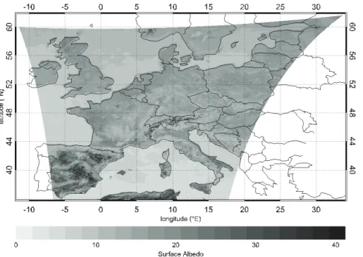
the background albedo map for our study domain is created by assigning to each pixel the minimum of the observed reflectance value over the entire study period. Figure 1 shows the map containingAobtained for June 2006, for our study domain.

Finally, in our implementation to retrieve SCOT we employ a scheme to discriminate, at every pixel of a SEVIRI image, between the liquid and ice water phases of the

10

cloud droplets. Ice versus water cloud discrimination is done using the ratio of the reflectances of the SEVIRI channels at 1.6 µm and 0.6 µm, respectively (Kidder and Vonder Haar, 1995; Kokhanovsky, 2006). Based on the study by Hutchison (1999), whenever this ratio is below a value of 0.7 we assume ice clouds, the cloud containing liquid water otherwise. In each case, the corresponding ice or liquid water LUT is used

15

to interpolateR₀∞(µ,µ₀,ϕ) from.

2.2 Estimation of surface UV irradiance

In order to obtain surface UV irradiance from the remotely sensed COT fields, we devel-oped a simple parameterization based on simulations performed with the Tropospheric Ultraviolet and Visible (TUV) radiative transfer model (Madronich, 1997), version 5.0.

20

TUV is a state-of-the-art model allowing to simulate, among others, the eff_{ect of clouds} on surface UV irradiance.

The TUV model is set up using the 8-stream discrete ordinates option. The surface albedo in the UV spectral range is set to 5%, which is consistent with values mentioned by Badosa et al. (2005), Kazantzidis et al. (2001), L ´opez et al. (2009), and Palancar

25

(9)

ACPD

12, 691–721, 2012

P. Pandey et al.

Title Page

Tables Figures

◭ ◮

Back Close

Full Screen / Esc

Discussion

P

a

per

|

Dis

cussion

P

a

per

|

Discussion

P

a

per

|

Discussio

n

P

a

per

|

spatial variability throughout this domain is very little. The columnar concentration val-ues for SO₂and NO₂are set to the TUV default values of 0 DU and also for aerosol pa-rameters default values are used: aerosol optical depth at 550 nm (τ_a=₀_._235), single-scattering albedo (ω₀=₀_._{99), and ˚}_{Angstr ¨om coe}ffi_{cient as unity. The value of cloud} asymmetry parameter (g) employed to calculate τ from the remotely sensed scaled

5

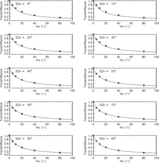
cloud optical thickness (τ∗) is set to 0.85, which is consistent with the TUV model. The TUV model is set up to calculate surface UV irradiance at sea level (10 m alti-tude) for diff_{erent cloud optical thickness values of}_τ=_{0, 5, 10, 20, 40 and 80, for solar} zenith angles (θ₀) ranging from 0◦to 90◦, in steps of 10◦.

Inspired by Fitzpatrick et al. (2004), the function, T(τ), to calculate transmission of

10

(broadband) solar radiation through clouds to modulate UV irradiance is given by:

T(τ)=a+bcosθ0

1+_cτ (6)

A fit between TUV-based results and the above empirical function is obtained fora=_1,

b=₀_._{0 and} _c=₀_._{075. The correspondence between our parameterisation and the} TUV-based results is excellent (Fig. 2).

15

The surface UV irradiance,E(τ,θ₀) is expressed as the product of the clear-sky value

E(0,θ₀) multiplied by the cloud transmissivity T(τ) as given in Eq. (6), yielding

E(τ,θ₀)=_E₍₀_,θ

0)T(τ) (7)

As the solar zenith angle is one of the most important parameter aff_{ecting the} sur-face UV levels (Lubin and Jensen, 1995), the clear-sky irradiance is parameterized as

20

a function of solar zenith angle employing the functional form proposed by Simpson et al. (2002), that is,

E(0,θ₀)=_E_τ₌₀_exp

γ

1− 1

cos(0.8θ₀)

(8)

The coeffi_cient_γ _{is estimated, based on TUV results, to be 1.95 and 3.55 for UV-A and} UV-B irradiance, respectively.

(10)

ACPD

12, 691–721, 2012

P. Pandey et al.

Title Page

Tables Figures

◭ ◮

Back Close

Full Screen / Esc

Discussion

P

a

per

|

Dis

cussion

P

a

per

|

Discussion

P

a

per

|

Discussio

n

P

a

per

|

The parameterization given by Eq. (7) is applied to time series of remotely sensed COT values for selected SEVIRI pixels, considering the same 15-min time intervals as those at which the cloud optical thickness is retrieved. In order to avoid the scattering phenomenon associated with lower solar elevation at the horizon and uncertainties in UV irradiance associated with it, the computation of surface UV irradiance levels is

5

limited to the pixels having solar zenith angle (θ₀) smaller than 77◦.

3 Results

3.1 Comparison of optical thickness with CloudSat

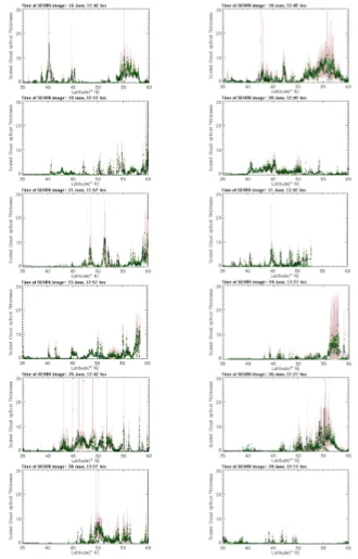
The methodology described in Sect. 2.1 was implemented on SEVIRI Level 1.5 daytime imagery to yield SCOT fields at 15-min intervals, for the month of June 2006. Figure 3

10

shows such fields at several selected instants corresponding to passes of the CloudSat instrument (Stephens et al., 2002), observations of which will be used to compare our results with.

CloudSat carries a 94-GHz cloud profiling radar, which yields cloud profile informa-tion, liquid and ice water content profiles, and precipitation. Optical thickness is

ob-15

tained by combining radar measurements with reflectances measured by the MODIS instrument onboard the Aqua platform, which flies in tandem with the CloudSat plat-form. As the CloudSat radar has a small field of view of approximately 1.4 km, and the platform being in a polar orbit, the data are confined to narrow tracks. Pixels within the tracks have a size of approximately 1.4 km×2.5 km, in the across- and along-track

20

directions, respectively. For the comparison, we used the CloudSat 2B-TAU cloud op-tical thickness product (CloudSat Project, 2008). However, since we derived SCOT, while the CloudSat 2B-TAU product contains (unscaled) COT, we converted the latter to SCOT by using an appropriate value of the asymmetry parameterg. In the genera-tion of the 2B-TAU product, use is made of a value ofg=₀_._{85 for water and}_g=₀_.₈₃₃₆

25

(11)

ACPD

12, 691–721, 2012

P. Pandey et al.

Title Page

Tables Figures

◭ ◮

Back Close

Full Screen / Esc

Discussion

P

a

per

|

Dis

cussion

P

a

per

|

Discussion

P

a

per

|

Discussio

n

P

a

per

|

adoptedg=₀_._{84 as a representative value for both the ice and liquid water phases.} SEVIRI-based SCOT results were interpolated to the positions of the CloudSat pixels along the tracks crossing our study domain (see Fig. 3). Figure 4 shows the result of the comparison between the SCOT values from SEVIRI versus those from CloudSat, along the track of the latter, for those times in June 2006 that a CloudSat track ran through

5

the study domain, hence corresponding to the images in Fig. 3. It is quite clear that the SEVIRI results match the CloudSat SCOT values rather well, most of the time being within the uncertainty range of the latter. Whenever extensive and thick clouds are present in the CloudSat data, our SEVIRI-based SCOT values properly identify those areas. Also, the absence of cloud is identified well by our approach, although a small

10

residual SCOT value is sometimes found in our results when CloudSat indicates the absence of cloud.

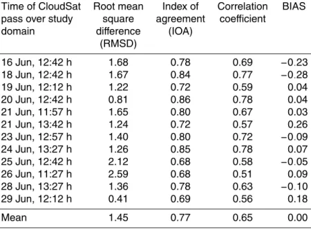
Table 1 quantifies the diff_{erence between the SEVIRI and CloudSat SCOT values for} each of the CloudSat tracks used. The bias, ranging between−0.28 to 0.26, is very low, without any general tendency towards systematically positive or negative values.

15

The root mean square diff_{erence (RMSD) is generally of the order of 1 to 2, which} is rather low compared to the typical SCOT values occurring in the CloudSat tracks considered here, reaching up to values of∼10 and beyond. The correlation between both sets of SCOT values is also reasonably good, in the range 0.51–0.78. Finally, the index of agreement also exhibits satisfactory values ranging between 0.68 and 0.86,

20

which points to a good performance of the retrieval scheme.

The SCOT values obtained from SACURA applied to SEVIRI are well within the un-certainty of the CloudSat values. The reason behind the diff_{erences in the SCOT can} be attributed to diff_{erences in the spatial resolution between the SEVIRI and CloudSat} pixels. A diff_{ering surface background albedo can also be associated with the}

discrep-25

ancies found in the SCOT.

(12)

ACPD

12, 691–721, 2012

P. Pandey et al.

Title Page

Tables Figures

◭ ◮

Back Close

Full Screen / Esc

Discussion

P

a

per

|

Dis

cussion

P

a

per

|

Discussion

P

a

per

|

Discussio

n

P

a

per

|

results obtained with SACURA applied to SCIAMACHY measurements, against results obtained based on MERIS and AATSR, also processed with the SACURA algorithm. The data obtained by these authors show correlation coeffi_{cients of 0.76 and 0.78, and} index of agreement (IOA) of 0.81 and 0.82, for MERIS and AATSR, respectively. As mentioned above, we obtained a mean correlation of 0.65 and mean IOA of 0.77 in

5

the comparison of our results with CloudSat. Any lesser performance of our approach may be explained by (1) diff_{erent algorithms used for SEVIRI and CloudSat (whereas} Kokhanovsky et al. (2007) used SACURA to measurements from both the MERIS and AATSR sensors), and (2) the mismatch between the pixels in the CloudSat track and the SEVIRI pixels, which is more severe than the spatial mismatch of SCIAMACHY

10

versus spatially aggregated MERIS respectively AATSR data.

The diff_{erence statistics we obtained for the results based on our approach versus} the CloudSat are reasonably satisfactory. This leads us to conclude that the application of SACURA algorithm to SEVIRI data yields satisfactory values for the scaled cloud optical thickness.

15

3.2 Comparison of surface UV irradiance with measurements

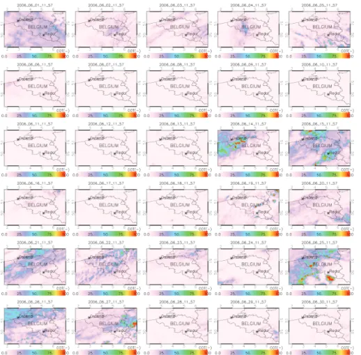
The resulting surface UV irradiance estimates computed by Eq. (7) were compared to measured values, obtained from UV monitoring stations located at Redu (50◦00′N, 5◦90′E) and Ostend (51◦14′N, 2◦56′E), both in Belgium, for the month of June 2006. Both stations have a fairly pristine atmosphere, as one is in a rural location and the

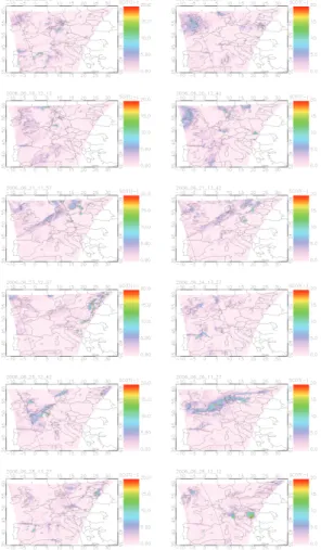
20

other is located at the Belgian coast, not experiencing pollution of an urban region. The location of Redu and Ostend can be seen from Fig. 5, which also shows the cloud optical thickness fields of each day at noon (11:57 UTC) of June 2006 as estimated from SEVIRI. In this figure, diff_{erent types of clouds – thin clouds, stratiform clouds,} scattered or broken clouds, thick to cumulonimbus clouds – are identifiable by means

25

(13)

ACPD

12, 691–721, 2012

P. Pandey et al.

Title Page

Tables Figures

◭ ◮

Back Close

Full Screen / Esc

Discussion

P

a

per

|

Dis

cussion

P

a

per

|

Discussion

P

a

per

|

Discussio

n

P

a

per

|

UVA-1 Pyranometer measures the global solar UV-A irradiance. The instrument uti-lizes colored glass filters and a UV-A sensitive phosphor screen to block all of the Sun’s visible light and convert the UV-A light into visible (green) light. A solid-state photodetector is employed in the instrument to measure the latter. The UVB-1 Pyra-nometer measures the global solar UV-B irradiance and utilizes the same technique as

5

that of UVA-1 Pyranometer. These instruments are regularly verified and recalibrated by means of National Institute of Standards and Technology (NIST) certified 1000 W Tungsten lamps. One measurement is taken every second by both the UV-meters. The data are recorded on a data-logger and averaged on 1-min intervals between 02:00 to 22:00 UT (04:00 to 24:00 local time) each day. The accuracy of the UV irradiance

10

measurements is estimated at±5 %.

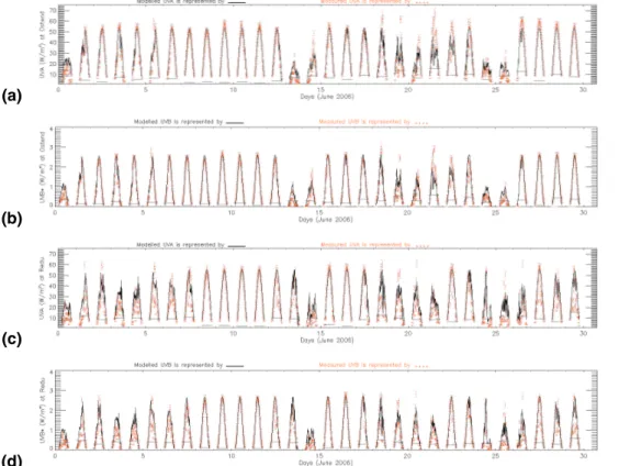
Figure 6 shows the estimated versus the observed surface UV-A and UV-B irradi-ance values for June 2006 at the selected stations. It is clear that the estimated values capture the temporal variation of the observations fairly well. In particular, the varia-tions between the obviously cloudy days versus the dominantly clear-sky periods are

15

reproduced well in the COT-based surface UV estimates. Moreover, the geographic dif-ferences between the stations are generally well captured, such as the systematically lower irradiances in the Redu station at the beginning and the end of the considered period, and related to the presence of enhanced cloud at that location. There are also days, though, mostly characterized by (nearly) clear sky conditions, on which the model

20

exhibits a low bias compared to the measurements. It has been reported that broken cloud decks or thin overcast cloud can enhance surface UV irradiance by up to several tens of percent, owing to light reflection at cloud edges and increased forward scatter-ing in certain cloud types (Calb ´o et al., 2005; Crawford et al., 2003). The enhancement observed in the measurements might be due to the diffuse component of the UV

radi-25

(14)

ACPD

12, 691–721, 2012

P. Pandey et al.

Title Page

Tables Figures

◭ ◮

Back Close

Full Screen / Esc

Discussion

P

a

per

|

Dis

cussion

P

a

per

|

Discussion

P

a

per

|

Discussio

n

P

a

per

|

most of the time the estimated UV irradiances match the observations well, often within the 5 % measurement error. Overall, the correspondence is slightly better for the UV-B than for the UV-A part of the spectrum.

The model versus measurement error statistics are shown in the Table 2. With the values of correlation varying from 0.88 to 0.91 for UV-A and UV-B, respectively, along

5

with index of agreement ranging between 0.91–0.97, it can be inferred that the pro-posed parameterisation is a good estimate of attenuation of UV-A and UV-B irradiance due to clouds. The RMSE values of the time series for Ostend and Redu for UV-A are 7.7 W m−2 and 9.07 W m−2, respectively, whereas, for UV-B it is 0.30 W m−2 and 0.36 W m−2, respectively. The variation of daily RMSE, shown by the horizontal line

10

in Fig. 6 indicates that the model and measurement values match well under clear sky condition. The influence of cloudy scenario, specially broken or transient clouds, somewhat deteriorates model performance for surface UV irradiance levels.

In addition to the above analysis, the conjunction of Figs. 6 and 5 also facilitates to comprehend the eff_{ect of clouds or absence of clouds on lower or higher surface UV}

15

irradiance levels, respectively.

4 Conclusions

This paper presents an application of the semi-analytical cloud retrieval algorithm (SACURA), designed for retrieving scaled cloud optical thickness, to MSG SEVIRI Level 1.5 reflectance imagery in the 0.6 µm channel and estimation of

correspond-20

ing surface UV irradiance. To illustrate model performance, a case study during the month of June 2006, for a domain covering a large part of Europe was analysed. To our best knowledge, this is the first application of SACURA to imagery obtained from a geostationary satellite platform to retrieve scaled cloud optical thickness (SCOT). The background (surface) albedo was determined from the reflectance imagery itself,

us-25

(15)

ACPD

12, 691–721, 2012

P. Pandey et al.

Title Page

Tables Figures

◭ ◮

Back Close

Full Screen / Esc

Discussion

P

a

per

|

Dis

cussion

P

a

per

|

Discussion

P

a

per

|

Discussio

n

P

a

per

|

the 0.6 µm reflectance values. The SCOT values obtained with SACURA from SEVIRI imagery were compared with values estimated by the CloudSat satellite. Overall, both methods gave very similar results, both in magnitude as in the spatial patterns, with an average root mean square diff_{erence of 1.45, index of agreement of 0.77, correlation} coeffi_{cient of 0.65 and null bias.}

5

Based on the retrieved cloud optical thickness values together with radiative transfer modelling approach, a simple parameterisation as a function of solar zenith angle and cloud optical thickness was proposed to yield the surface level UV-A and UV-B irradi-ance. The estimated surface level UV-A and UV-B irradiance were validated against measurements over two Belgian stations, Redu and Ostend, for the same period of

10

June 2006. The correlation between measurements and model results were found to be in the range of 0.88 to 0.91. The index of agreement varied between 0.91–0.97. A low bias was found between measurements and model results. A satisfactory mod-elled versus measured surface UV, UV-A and UV-B, irradiance leads to the conclusion that the proposed approach is competent in estimating the surface UV irradiance by

15

(16)

ACPD

12, 691–721, 2012

P. Pandey et al.

Title Page

Tables Figures

◭ ◮

Back Close

Full Screen / Esc

Discussion

P

a

per

|

Dis

cussion

P

a

per

|

Discussion

P

a

per

|

Discussio

n

P

a

per

|

List of symbols

Symbol Description Units

I_λ Radiance W m−2sr−1(cm−1)−1

Φ _Latitude _Degree

Ω _Longitude _Degree

τ Cloud optical depth –

τ∗ Scaled cloud optical depth –

g Asymmetry parameter –

θ₀ Solar zenith angle Degrees

θ Satellite zenith angle Degrees

υ0 Solar azimuth angle Degrees

υ Satellite azimuth angle Degrees

ϕ Relative azimuth angle Degrees

δ Solar declination angle Degrees

R₀∞ Reflectance of semi-infinite cloud –

R Observed reflectance –

K(µ) Escape function –

t Global transmittance –

T Solar broadband transmittance –

(17)

ACPD

12, 691–721, 2012

P. Pandey et al.

Title Page

Tables Figures

◭ ◮

Back Close

Full Screen / Esc

Discussion

P

a

per

|

Dis

cussion

P

a

per

|

Discussion

P

a

per

|

Discussio

n

P

a

per

|

Appendix A

Solar – satellite angles

A1 Solar zenith angle

The solar zenith angle (θ₀) is given as following:

5

θ₀=_cos−1_(sin_φ_sin_δ+_cos_φ_cos_δ_cosH

a) (A1)

withφthe latitude of the considered pixel’s position, and

δ=₋₂₃_._45cos2π(JD+10)

365 (A2)

the solar declination angle, which depends on the Julian Day (JD). The hour angle is given by

10

H_a=₁₅₍_l₋₁₂₎_, _(A3)

with the local (solar) apparent time given by

l=_time+ Ω +_X

time.

In this last expressiontimerefers to the UTC time (in hours),Ω_{is longitude (in degrees),} and

15

X_time=₉_._87sin2_β₋₇_._53cos_β₋₁_._5sin_β _(A4) is the equation of time, withβ=₂_π_(JD₋₈₁₎_/_365.

A2 Solar-satellite azimuth angles

The solar azimuth angle (ν₀) is given as (Kidder and Vonder Haar, 1995),

ν₀=_cos−1

_cos_H

acosδsinΦ−sinδcosΦ

sinθ₀

(A5)

(18)

ACPD

12, 691–721, 2012

P. Pandey et al.

Title Page

Tables Figures

◭ ◮

Back Close

Full Screen / Esc

Discussion

P

a

per

|

Dis

cussion

P

a

per

|

Discussion

P

a

per

|

Discussio

n

P

a

per

|

Assuming a spherical earth, the radius vector extending from the centre of the Earth to the considered pixel,r_e, is given as

r_e=





r_ecosΦ_cosΩ

r_ecosΦsinΩ

r_esinΦ



 (A6)

Similarly,r_s the radius vector of the satellite is given by

r_s=





dvcosΦ0cosΩ0 d_vcosΦ₀_sinΩ₀

dvsinΦ0 

 (A7)

5

whereΦ₀=₀◦_{, is sub satellite latitude.}

The diff_{erence vector being defined by,} _r_d_≡_r_s₋_r_e_{, the}_{satellite zenith angle}₍_θ_{), as} described by Kidder and Vonder Haar (1995), is given by

θ=_cos−1

_r

s·rd |r_s||r_d|

. (A8)

To calculate thesatellite azimuth angle(ν), we employ two vectors in the tangent plane

10

at the observational point. Again following Kidder and Vonder Haar (1995), the first vector pointing north,r_N, is given as

r_N=





−sinΦ_cosΩ

−sinΦ_sinΩ cosΦ



. (A9)

The second vector,r_H, is the horizontal projection ofr_dgiven by

r_H=_r

d−rd

r_e

|r_e|cosθ (A10)

(19)

ACPD

12, 691–721, 2012

P. Pandey et al.

Title Page

Tables Figures

◭ ◮

Back Close

Full Screen / Esc

Discussion

P

a

per

|

Dis

cussion

P

a

per

|

Discussion

P

a

per

|

Discussio

n

P

a

per

|

From Eqs. (A9) and (A10) we obtain thesatellite azimuth angle

ν=_cos−1

_r

N·rH |r_N||r_H|

. (A11)

The next parameter calculated is therelative azimuth angle(φ)

φ=₍_ν₋_ν

0)+π (A12)

We assume that therelative azimuth angleis equal to πwhen sun and satellite are in

5

the same line and sun is shining from behind the satellite, as described by Capderou (2005).

Acknowledgement. We are grateful to Alexander Kokhanovsky, Institute of Environmental Physics, Bremen University, Bremen, Germany, for his valuable guidance and suggestions in carrying out this work. We are thankful to EUMETSAT for providing us SEVIRI data. We are

10

also thankful to CloudSat community for availability of data and their description. We acknowl-edge also the support by the Climate and air quality modeling for policy support (CLIMAQS) project together with Promote air quality services integrating observations development of basic localised information for Europe (PASODOBLE) projects.

References

15

Alados-Arboledas, L., Alados, I., Foyo-Moreno, I., Olmo, F. J., and Alc ´antara, A.: The influence of clouds on surface UV erythemal irradiance, Atmos. Res., 66, 273–290, 2003.

Badosa, J., Gonz ´alez, J., and Calb ´o, J.: Using a parameterization of a radiative transfer model to build high-resolution maps of typical clear-sky UV index in Catalonia, Spain, J. Appl. Me-teorol., 44, 789–803, 2005.

20

Baum, B., Yang, P., Heymsfield, A., and Thomas, S.: Bulk scattering properties for the remote sensing of ice clouds. Part I: Microphysical data and models, J. Appl. Meteorol., 44, 1885– 1895, 2005.

Calb ó, J., Pag ès, D., and Gonz ález, J.: Empirical studies of cloud eff_{ects on UV radiation:}

a review, Rev. Geophys., 2005.

(20)

ACPD

12, 691–721, 2012

P. Pandey et al.

Title Page

Tables Figures

◭ ◮

Back Close

Full Screen / Esc

Discussion

P

a

per

|

Dis

cussion

P

a

per

|

Discussion

P

a

per

|

Discussio

n

P

a

per

|

Capderou, M.: Satellites-Orbits and Missions, Springer, 2005.

CloudSat project: CloudSat Standard Data Products Handbook, 2008.

Crawford, J., Shetter, R., Lefer, B., Cantrell, C., Junkermann, W., Madronich, S., and Calvert, J.: Cloud impacts on UV spectral actinic flux observed during the International Photolysis Fre-quency Measurement and Model Intercomparison (IPMMI), J. Geophys. Res., 108(D16),

5

8545, 2003.

Estupinan, J. G., Raman, S., Crescenti, G. H., Streicher, J. J., Barnard, W. F.: Eff_{ects of clouds}

and haze on UV-B radiation, J. Geophys. Res., 101(D11), 16807–16816, 1996.

EUMETSAT, MSG ground segment LRIT/HRIT mission specific implementation, EUM/MSG/SPE/057 (2006), Darmstadt, Germany.

10

Fitzpatrick, M. F., Brandt, R. E., and Warren, G. S.: Transmission of solar radiation by clouds over snow and ice surfaces: a parameterization in terms of optical depth, solar zenith angle, and surface albedo, J. Climate, 17, 266–275, 2004.

Gieske, A. S. M., Hendrikse, J. H. M., Retsios, V., Leeuwen, B. V., Maathuis, B. H. P., Roma-guera, B., Sobrino, J. A., Timmermans, W. J., and Su, Z.: Processing of MSG-1 SEVIRI

15

data in the thermal infrared-algorithm development with the use of the SPARC2004 data set, Proceedings of the ESA WPP-250: SPARC Final Workshop, 4–5 July, 2005, Enschede, ESA.

Govaerts, Y. M., Arriaga, A., and Schmetz, J.: Operational vicarious calibration of the MSG/SEVIRI solar channels, Adv. Space Res., 28, 21–30, 2001.

20

Graeme, L. S. and Kummerow, C. D.: The remote sensing of clouds and precipitation from space: a review, J. Atmos. Sci., 64, 3742–3765, 2007.

Hutchison, K. D.: Application of AVHRR/3 imagery for the improved detection of thin cirrus clouds and specification of cloud-top phase, J. Atmos. Ocean. Technol., 16, 1885–1899, 1999.

25

Jourdan, O., Oshchepkov, S., Shcherbakov, V., Gayet, J. F., and Isaka, H.: Assessment of cloud optical parameters in the solar region: retrievals from airborne measurements of scattering phase functions, J. Geophys. Res., 108(D18), 4572, 2003.

Kahn, B. H., Chahine, M. T., Stephens, G. L., Mace, G. G., Marchand, R. T., Wang, Z., Bar-net, C. D., Eldering, A., Holz, R. E., Kuehn, R. E., and Vane, D. G.: Cloud type comparisons

30

of AIRS, CloudSat, and CALIPSO cloud height and amount, Atmos. Chem. Phys., 8, 1231-1248, doi:10.5194/acp-8-1231-2008, 2008.

(21)

ACPD

12, 691–721, 2012

P. Pandey et al.

Title Page

Tables Figures

◭ ◮

Back Close

Full Screen / Esc

Discussion

P

a

per

|

Dis

cussion

P

a

per

|

Discussion

P

a

per

|

Discussio

n

P

a

per

|

satellite retrieved cloud optical thickness: marine stratocumulus case, J. Geophys. Res., 114, D01202, 2009.

Kazantzidis, A., Balis, D. S., Bais, A. F., Kazadis, S., Galani, E., and Kosmidis, E.: Comparison of model caloculations with spectral UV measurements during the SUSPEN campaign: the eff_{ects of aerosols, J. Atmos. Sci., 58, 1529–1539, 2001.}

5

Kidder, S. Q. and Von der Haar, T. H.: Satellite Meteorology – An Introduction, Academic Press, United Kingdom, 1995.

King, M. D.: Details of scaled optical thickness of cloud from reflected solar radiation measure-ments, J. Atmos. Sci., 44, 1734–1751, 1987.

King, M. D., Kaufman, Y. J., Menzel, W. P., and Tanr ´e, D.: Remote sensing of cloud, aerosol,

10

and water vapor properties from the Moderate Resolution Imaging Spectrometer (MODIS), IEEE Trans. Geosci. Remote Sensing, 30, 1992.

Kokhanovsky, A. A.: Cloud Optics, Springer, Netherlands, 2006.

Kokhanovsky, A. A. and Nauss, T.: Satellite-based retrieval of ice cloud properties using a semi-analytical algorithm, J. Geophys. Res., 110, D19206, 2005.

15

Kokhanovsky, A. A., Rozanov, V. V., Zege, E. P., Bovesmann, H., and Burrows, J. P.: A semi an-alytical cloud retrieval algorithm usinfg backscattered radiation in 0.4–2.4 µm spectral region, J. Geophys. Res., 108(D1), 4008, 2003.

Kokhanovsky, A. A., Nauss, T., Schreier, M., Huene, W. V. H., and Burrows, J. P.: The intercom-parison of cloud parameters derived using multiple satellite instruments, IEEE Trans. Geosci.

20

Remote Sensing, 45, 1, 2007.

Kudish, A. I. and Evseev, E.: Statistical relationships between solar UVB and UVA radiation and global radiation measurements at two sites in Israel, Int. J. Climatol., 20(7), 759–770, 2000.

L ´opez, M. L., Palancar, G. G., and Toselli, B. M.: Eff_{ect of di}ff_{erent types of clouds on surface} 25

UV-B and total solar irradiance at southern mid-latitudes: CMF determinations at C ´ordoba, Argentina, Atmos. Environ., 43, 3130–3136, 2009.

Lin, X., Randall, D. A., and Fowler, L.: Diurnal variability of the hydrologic cycle and radiative fluxes: comparisons between observations and a GCM, J. Climate, 13, 4159–4179, 2000. Lubin, D. and Jensen, E. H.: Eff_{ects of clouds and stratospheric ozone depletion on ultraviolet} 30

radiation trend, Nature, 377, 710–713, 1995.

Madronich, S.: Photodissociation in the atmosphere actinic flux and the eff_{ects of ground}

(22)

ACPD

12, 691–721, 2012

P. Pandey et al.

Title Page

Tables Figures

◭ ◮

Back Close

Full Screen / Esc

Discussion

P

a

per

|

Dis

cussion

P

a

per

|

Discussion

P

a

per

|

Discussio

n

P

a

per

|

Madronich, S. and Flocke, S.: Theoretical estimation of biologically eff_{ective UV radiation at}

the Earth’s surface, in: Solar Ultraviolet Radiation – Modeling, Measurements and Eff_ects,

edited by: Zerefos, C., NATO ASI Series Vol. I52, Springer-Verlag, Berlin, 1997.

Mateos, D., Sarra, A., Meloni, D., Biagio, C. D., and Sferlazzo, D. M.: Experimental determina-tion of cloud influence on the spectral UV irradiance and implicadetermina-tions for biological eff_{ects, J.} 5

Atmos. Solar-Terrestrial Phys., 73(13), 1739–1746, 2011.

Monks, P. S., Rickard, A. R., Hall, S. L., and Richards, N. A. D.: Attenuation of spectral actinic flux and photolysis frequencies at the surface through homogenous cloud fields, J. Geophys. Res., 109, D17206, 2004.

Moreno, I. F., Alados, I., Olmo, F. J., and Arboledas, L. A.: The influence of cloudiness on UV

10

global irradiance (295–385 nm), Agric. Forest Meteorol., 120, 101–111, 2003. MSG Level 1.5 image data format description (August 2007), EUMETSAT.

Nakajima, T. and King, M. D.: Determination of optical thickness and eff_{ective radius of clouds}

from reflected solar radiation measurements, Part I: Theory, J. Atmos. Sci., 47, 1878–1893, 1990.

15

Nauss, T. and Kokhanovsky, A. A.: Retrieval of warm cloud optical thickness using simple approximations, Remote Sensing Environ., 115, 1317–1325, 2011.

Nauss, T., Kokhanovsky, A. A., Nakajima, T. Y., Reudenbach, C., and Bendix, J.: The intercom-parison of selected cloud retrieval algorithms, Atmos. Res., 78, 46–78, 2005.

Palancar, G. G., Shetter, R. E., Hall, S. R., Toselli, B. M., and Madronich, S.: Ultraviolet actinic

20

flux in clear and cloudy atmospheres: model calculations and aircraft-based measurements, Atmos. Chem. Phys., 11, 5457–5469, doi:10.5194/acp-11-5457-2011, 2011.

Roebeling, R. A., Feijt, A. J., and Stammes, P.: Cloud property retrievals for climate monitoring: implications of differences between Spinning Enhanced Visible and Infrared Imager (SEVIRI) on METEOSAT-8 and Advanced Very High Resolution Radiometer (AVHRR) on NOAA-17,

25

J. Geophys. Res., 111, D20210, 2006.

Saburg, J. M. and Parisi, A. V.: Spectral dependency of cloud enhanced UV irradiance, Atmos. Res., 81, 206–214, 2006.

Seckmeyer, G., Erb, R., and Albold, A.: Transmittance of a cloud is wavelength-dependent in the UV-range, J. Geophys. Res., 23, 2753–2755, 1996.

30

Simpson, W. R., King, M. D., Beine, H. J., Honrath, R. E., and Peterson, M. C.: Atmospheric photolysis rate coeffi_{cients during the Polar Sunrise Experiment ALERT2000, Atmos.}

(23)

ACPD

12, 691–721, 2012

P. Pandey et al.

Title Page

Tables Figures

◭ ◮

Back Close

Full Screen / Esc

Discussion

P

a

per

|

Dis

cussion

P

a

per

|

Discussion

P

a

per

|

Discussio

n

P

a

per

|

Stephens, G. L., Vane, D. G., Boain, R. J., Mace, G. G., Sassen, K., Wang, Z., Illingworth, A. J., O’Connor, E. J., Rossow, W. B., Durden, S. L., Miller, S. D., Austin, R. T., Benedetti, A., Mitrescu, C., and the CloudSat Science Team: The CloudSat mission and the A-Train: a new dimension of space-based observations of clouds and precipitation, B. Am. Meteorol. Soc., 83, 1771–1790, 2002.

5

V ´azquez, M. and Hanslmeier, A.: Ultraviolet Radiation in the Solar System, Springer, The Netherlands, 2006.

van der A, R. J., Allaart, M. A. F., and Eskes, H. J.: Multi sensor reanalysis of total ozone, Atmos. Chem. Phys., 10, 11277–11294, doi:10.5194/acp-10-11277-2010, 2010.

Van der Leun, J. C., Tevini, M., and Worrest, R. C. (Eds.): Environmental Eff_{ects of Ozone} 10

Depletion: 1998 Update. United Nations Environmental Programme, Nairobi, 1998.

Wolters, E. L., Roebeling, R. A., and Feijt, A. J.: Evaluation of cloud-Phase Retrieval Meth-ods for SEVIRI on Meteosat-8 Using Ground-Based Lidar and Cloud Radar Data, J. Appl. Meteorol. Climatol., 47, 1723–1738, 2008.

Zhang, Z., Yang, P., Kattawar, G., Riedi, J., Labonnote, L. C., Baum, B. A., Platnick, S., and

15

(24)

ACPD

12, 691–721, 2012

P. Pandey et al.

Title Page

Tables Figures

◭ ◮

Back Close

Full Screen / Esc

Discussion

P

a

per

|

Dis

cussion

P

a

per

|

Discussion

P

a

per

|

Discussio

n

P

a

per

|

Table 1.Error statistics between estimated SCOT from SEVIRI and SCOT from CloudSat.

Time of CloudSat Root mean Index of Correlation BIAS pass over study square agreement coefficient

domain diff_erence _(IOA)

(RMSD)

16 Jun, 12:42 h 1.68 0.78 0.69 −0.23 18 Jun, 12:42 h 1.67 0.84 0.77 −0.28 19 Jun, 12:12 h 1.22 0.72 0.59 0.04 20 Jun, 12:42 h 0.81 0.86 0.78 0.04 21 Jun, 11:57 h 1.65 0.80 0.67 0.03 21 Jun, 13:42 h 1.24 0.72 0.57 0.26 23 Jun, 12:57 h 1.40 0.80 0.72 −0.09 24 Jun, 13:27 h 1.26 0.85 0.78 0.07 25 Jun, 12:42 h 2.12 0.68 0.58 −0.05 26 Jun, 11:27 h 2.59 0.68 0.51 0.09 28 Jun, 13:27 h 1.36 0.78 0.63 −0.10 29 Jun, 12:12 h 0.41 0.69 0.56 0.18

(25)

ACPD

12, 691–721, 2012

P. Pandey et al.

Title Page

Tables Figures

◭ ◮

Back Close

Full Screen / Esc

Discussion

P

a

per

|

Dis

cussion

P

a

per

|

Discussion

P

a

per

|

Discussio

n

P

a

per

|

Table 2.Error statistics between estimated surface level UV irradiance and measurements.

Quantity Station Root mean Index of Correlation BIAS square agreement coeffi_cient

error (IOA) (RMSE)

(26)

ACPD

12, 691–721, 2012

P. Pandey et al.

Title Page

Tables Figures

◭ ◮

Back Close

Full Screen / Esc

Discussion

P

a

per

|

Dis

cussion

P

a

per

|

Discussion

P

a

per

|

Discussio

n

P

a

per

|

(27)

ACPD

12, 691–721, 2012

P. Pandey et al.

Title Page

Tables Figures

◭ ◮

Back Close

Full Screen / Esc

Discussion

P

a

per

|

Dis

cussion

P

a

per

|

Discussion

P

a

per

|

Discussio

n

P

a

per

|

(28)

ACPD

12, 691–721, 2012

P. Pandey et al.

Title Page

Tables Figures

◭ ◮

Back Close

Full Screen / Esc

Discussion

P

a

per

|

Dis

cussion

P

a

per

|

Discussion

P

a

per

|

Discussio

n

P

a

per

|

(29)

ACPD

12, 691–721, 2012

P. Pandey et al.

Title Page

Tables Figures

◭ ◮

Back Close

Full Screen / Esc

Discussion

P

a

per

|

Dis

cussion

P

a

per

|

Discussion

P

a

per

|

Discussio

n

P

a

per

|

(30)

ACPD

12, 691–721, 2012

P. Pandey et al.

Title Page

Tables Figures

◭ ◮

Back Close

Full Screen / Esc

Discussion

P

a

per

|

Dis

cussion

P

a

per

|

Discussion

P

a

per

|

Discussio

n

P

a

per

|

(31)

ACPD

12, 691–721, 2012

P. Pandey et al.

Title Page

Tables Figures

◭ ◮

Back Close

Full Screen / Esc

Discussion

P

a

per

|

Dis

cussion

P

a

per

|

Discussion

P

a

per

|

Discussio

n

P

a

per

|

(a)

(b)

(c)

(d)