www.atmos-chem-phys.net/11/7817/2011/ doi:10.5194/acp-11-7817-2011
© Author(s) 2011. CC Attribution 3.0 License.
Chemistry
and Physics
Radon activity in the lower troposphere and its impact on ionization
rate: a global estimate using different radon emissions
K. Zhang1,*, J. Feichter1, J. Kazil2,9, H. Wan1, W. Zhuo3, A. D. Griffiths4, H. Sartorius5, W. Zahorowski4, M. Ramonet6, M. Schmidt6, C. Yver6, R. E. M. Neubert7, and E.-G. Brunke8
1Max Planck Institute for Meteorology, Hamburg, Germany
2Cooperative Institute for Research in Environmental Sciences (CIRES), University of Colorado, Boulder, Colorado, USA 3Institute of Radiation Medicine, Fudan University, Shanghai, China
4Australian Nuclear Science and Technology Organisation, Lucas Heights NSW 2234, Australia 5Federal Office for Radiation Protection (BfS), Salzgitter, Germany
6Laboratoire des Sciences du Climat et de l’Environnement, IPSL, CEA, UVSQ, CNRS, Gif-sur-Yvette, France 7Centre for Isotope Research, University of Groningen, Groningen, The Netherlands
8South African Weather Service, Stellenbosch, South Africa
9NOAA Earth System Research Laboratory (ESRL), Boulder, Colorado, USA *now at: Pacific Northwest National Laboratory, Richland, Washington, USA
Received: 16 October 2010 – Published in Atmos. Chem. Phys. Discuss.: 28 January 2011 Revised: 15 July 2011 – Accepted: 1 August 2011 – Published: 3 August 2011
Abstract. The radioactive decay of radon and its progeny can lead to ionization of air molecules and consequently influence aerosol size distribution. In order to provide a global estimate of the radon-related ionization rate, we use the global atmospheric model ECHAM5 to simulate trans-port and decay processes of the radioactive tracers. A global radon emission map is put together using regional fluxes re-ported recently in the literature. Near-surface radon concen-trations simulated with this new map compare well with mea-surements.
Radon-related ionization rate is calculated and compared to that caused by cosmic rays. The contribution of radon and its progeny clearly exceeds that of the cosmic rays in the mid-and low-latitude lmid-and areas in the surface layer. During cold seasons, at locations where high concentration of sulfuric acid gas and low temperature provide potentially favorable conditions for nucleation, the coexistence of high ionization rate may help enhance the particle formation processes. This suggests that it is probably worth investigating the impact of radon-induced ionization on aerosol-climate interaction in global models.
Correspondence to:K. Zhang (kai.zhang@pnnl.gov)
1 Introduction
In recent years the impact of atmospheric ions on aerosol formation and life cycle has attracted increasing attention (see, e.g., Yu and Turco, 2000; Lovejoy et al., 2004; Kulmala et al., 2004; Kazil et al., 2006, among others). Atmospheric ions can enhance the production of ultrafine aerosol particles because they greatly stabilize small clusters against evapo-ration (Ramamurthi et al., 1993; Lovejoy et al., 2004). In addition, ions can attach to existing aerosol particles (either neutral or charged), change their charge status, and thus the coagulation rates (Clement and Harrison, 1992). Through influence on aerosol number and size distribution, ions can eventually exert an impact on the Earth’s climate. Kazil et al. (2010) show that in the global aerosol-climate model ECHAM5-HAM, charged H2SO4/H2O nucleation induces a −1.15 W m−2 (global and annual mean) flux of shortwave
radiation at the top of the atmosphere via direct, semi-direct and indirect aerosol effects. This value is considerably larger than the fluxes caused by cluster activation (−0.235 W m−2) and neutral H2SO4/H2O nucleation (−0.05 W m−2). In that
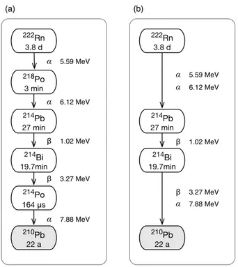
!!! "# $%&'( !)&*+ $',-# !).*/ !0',-# !). 1-)2%0,-# !). *+ )3.'!4
!)5 */ !!'6 5.59 MeV 6.12 MeV 1.02 MeV 3.27 MeV 7.88 MeV (a) !!! "# $%&'( !).*/ !0',-# !). 1-)2%0,-# !)5 */ !!'6 (b) α β β α α 5.59 MeV 6.12 MeV 1.02 MeV 3.27 MeV 7.88 MeV α β β α α
Fig. 1. (a)Radioactive decay of radon and its progeny. The half-life, decay type and decay energy of each species are also listed.(b) The simplified decay chain considered in our simulations.
their progeny, as well as terrestrial gamma radiation (Harri-son and Carslaw, 2003). Near the land surface, almost half of the ionization of the air is related to radon, thoron and their daughter products (Emsley, 2001).
Radon, the decay product of226Ra, is the most prominent natural radionuclide in the surface air. It is a noble gas with very low solubility in water. After being transpired into the air, radon can be redistributed into the middle and upper tro-posphere and over synoptic distance in the horizontal, due to its half-life of 3.8 days. The radioactive decay of222Rn
and its progeny produces highly energeticαandβ particles which ionize air molecules (Fig. 1a). A previous laboratory study by Vohra et al. (1984) showed that under typical near-surface conditions over land, ionization caused by radioac-tive decay of radon series can cause significant enhancements in particle formation. To find out whether it is necessary to consider radon-related nucleation in global aerosol models, we use the global climate model ECHAM5 to compare the radon-related ionization rate with that caused by cosmic rays. In order to obtain a realistic estimate of radon-related ionization rate, one needs sufficiently accurate information about radon emission flux on the global scale, as well as a nu-merical model that reasonably represents radon-related trans-port and decay processes. To this end a new global emission map is compiled in this study, and the transport processes in the ECHAM5 model are evaluated. The details are presented in Sects. 2 and 3. The simulated radon-related ionization rate is discussed in Sect. 4. Conclusions are drawn in Sect. 5.
2 Model, emission data, and simulations
In this section we first explain why we only choose radon and its progeny as ionization agents in this study. Thereafter the newly derived global radon emission map is presented (Sect. 2.2). We then briefly introduce the ECHAM5 model (Sect. 2.3) and document how radioactive decay and the re-sulting ionization are implemented in the model (Sects. 2.4, 2.5, and 2.6). The numerical simulations are introduced in Sect. 2.7.
2.1 Ionization agents
Since our primary interest lies in climate modelling on the global scale, the focus of this study was chosen by two cri-teria: first, the source of ionizing energy has to be strong enough to cause a globally non-negligible effect; Second, sufficient information needs to be available about the global distribution of the radionuclide and its sources, so that robust results can be obtained with our climate model. According to these criteria, we have chosen the radon decay series as the subject in this study.
Here we have deliberately excluded other well-known ra-dionuclides for various reasons. For example,85Kr has a long lifetime and fairly homogeneous background concentration worldwide, which makes it a continuous source of ioniza-tion. Over the ocean, its activity concentration can exceed that of radon. However, the decay energy of85Kr is rela-tively low (mainlyβdecay, average energy 0.251 MeV), and the activity concentration near land surface is much lower than radon. The resulting ionization in the lower troposphere is thus probably negligible compared to radon and cosmic rays. Similarly, ionization caused by14C in CO
2is neglected
due to its low decay energy (0.156 MeV) and low activity concentration (40 mBq m−3). The thoron decay chain could
have been another potential subject for our study. Although thoron (220Rn) and its direct daughter216Po undergo essen-tially complete decay below an altitude of several meters over land (with half-lives being 56 s and 0.15 s, respectively), the next decay product,212Pb, has a half-life of 10.6 h. However, it should be noted that the activity concentration of212Pb is only about 1 %–10 % of that of radon. Moreover, there exists the practical difficulty that information about thoron emis-sion is very limited. To our knowledge there is no global map available, which prevents us from obtaining reliable distribu-tions of thoron and its progeny. Given all the consideradistribu-tions above, we focus only on the radon-induced ionization in this study.
2.2 Radon emission
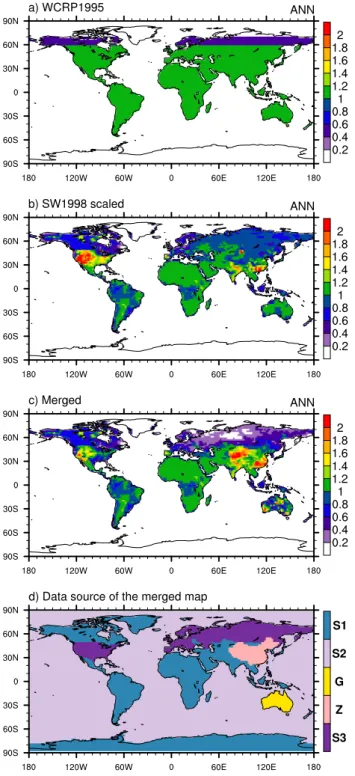
Fig. 2. (a–c) Radon emission setups considered in this study. The quantity shown is the annual mean atom number flux (unit: atom cm−2s−1). (d) Data source of the merged emission map shown in(c). S1 stands for Schery and Wasiolek (1998) (scaled), S2 for Schery and Huang (2004), G for Griffiths et al. (2010), Z for Zhuo et al. (2008), and S3 for Szegvary et al. (2007).
Table 1.Regionally averaged annual mean radon emission flux over land in the merged radon flux map.
Region Emission Flux
(atom cm−2s−1)
Europe 0.62
China 1.41
Russia 0.39
USA 0.87
Australia 1.02
Others 0.92
Global (between 60◦S and 60◦N) 0.96
in model intercomparison studies. For example, the World Climate Research Program (WCRP) Cambridge Workshop of 1995 (Rasch et al., 2000) specified a uniform con-tinental emission of 1 atom cm−2s−1 between 60◦S and 60◦N, 0.5 atom cm−2s−1between 60◦N and 70◦N (exclud-ing Greenland), and zero flux elsewhere. On the other hand, Lee and Feichter (1995) and Guelle et al. (1998) showed that taking into account regional gradient can lead to results more consistent with the observed radon concentrations, especially near the surface and at high latitudes. Conen and Robertson (2002) proposed a northward decreasing source (linear de-crease from 1 atom cm−2s−1at 30◦N to 0.2 atom cm−2s−1
at 70◦N) without zonal gradient. This emission assumption was tested with a global transport model by Robertson et al. (2005). Before our work presented in this paper, the global radon flux map by Schery and Wasiolek (1998) (hereafter SW1998) was the only one that includes detailed regional in-formation and seasonal variation over land surfaces. It has been used in several studies of transport modelling (see, e.g., Koch et al., 2006; Hirao et al., 2008). (Goto et al. (2008) showed limited results from a radon exhalation rate distri-bution model, but without comprehensive evaluation.) One of the weak points of the SW1998 map is the lack of over-all normalization. The annual and global mean emission rate over land (1.6 atom cm−2s−1) is higher than that given by
many previous estimates (Schery and Wasiolek, 1998; Sch-ery, 2004). Thus it is suggested (Schery 2009, personal com-munication) that one could let the overall normalization be a free parameter. For example, Koch et al. (2006) arbitrarily reduced the emission by a factor of 0.5 in their work.
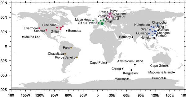
Fig. 3. Location of surface radon measurements used in this study. See Table 2 for further information of the sites. Colors indicate observational sites in the five different regions that are analysed separately in Fig. 5.
as well. Zhuo et al. (2008) published radon emission esti-mates for China based on the soil226Ra content and a global ecosystems database. The annual mean values given by their idealized model range from 0.5 to 2.7 atom cm−2s−1at dif-ferent locations. Furthermore, Griffiths et al. (2010) reported a time-dependent map of radon flux density at high resolu-tions for Australia. For the oceans, Schery and Huang (2004) calculated radon flux from the surface wind speed and sea water226Ra content using a gas transfer model.
Based on the studies mentioned above, we compile a new global radon emission map in this work (Fig. 2). The new map uses the Szegvary et al. (2007) data for Europe, Rus-sia and USA, Zhuo et al. (2008) for China, Griffiths et al. (2010) for Australia (pre-release), and the Schery and Wasi-olek (1998) map for other land areas but scaled by a factor of
1
1.6. The Schery and Huang (2004) estimates are used for the
oceans. Table 1 shows the annual mean regionally averaged radon emission flux over land in this merged map. For in-tercomparison, simulations are performed using this merged map, the WCRP1995 recommendation, and the scaled (also by a factor of 11.6) SW1998 map. The decision of using 11.6 for the normalization instead of 2 as in Koch et al. (2006) is somewhat arbitrary. The idea is that 11.6 results in a land-surface mean of 1 atom cm−2s−1, which is the value used for middle and low latitudes in the WCRP1995 protocol. On the other hand, we do not make it a strict rule that all three simulations must have the same global mean emission. 2.3 The climate model ECHAM5
ECHAM5 (Roeckner et al., 2003) is an atmospheric general circulation model developed at the Max Planck Institute for
Meteorology. Its spectral transform dynamical core solves the primitive equations in vorticity-divergence form. The horizontal resolution used in this study is T63, which applies a triangular truncation to the spherical harmonic series, and resolves horizontal patterns up to wave number 63. The cor-responding Gaussian grid, on which the grid-point computa-tions including physics parameterizacomputa-tions are performed, has approximately 2◦(latitude)×2◦(longitude) grid size. In the vertical, the model domain is unevenly divided into 31 layers in pressure-based terrain following coordinate, with the high-est computational level located at 10 hPa. Roughly speaking, there are 6 layers below 850 hPa, 9 above 200 hPa, and 16 in between. The standard time step for this model resolution is 12 min.
The large-scale advection of tracer species is handled by the Lin and Rood (1996) flux-form semi-Lagrangian algo-rithm, assuming piecewise parabolic sub-grid distribution. Within the physics parameterization package, the turbulent surface fluxes are calculated from the Monin-Obukhov simi-larity theory (Louis, 1979). Vertical diffusion coefficients are calculated as functions of turbulent kinetic energy (Brinkop and Roeckner, 1995). The parameterization of cumulus con-vection and convective transport of tracer is based on the bulk mass flux concept of Tiedtke (1989), with further modifica-tions by Nordeng (1994).
2.4 Decay of the radon family in the model
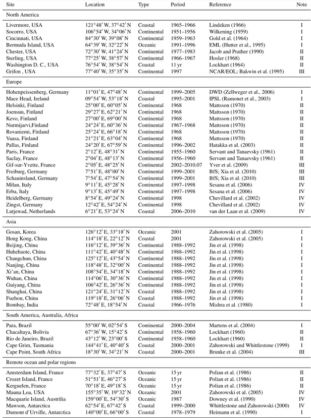
Table 2. Detailed information about the surface radon measurements used in this study. In the “Reference” column, DWD stands for Deutscher Wetterdienst (German Weather Service), BfS for Federal Office for Radiation Protection of Germany, IPSL for Institut Pierre-Simon Laplace, EML for DOE/Environmental Measurements Laboratory, and NCAR/EOL for National Center for Atmospheric Research Earth Observing Laboratory. The right most column categorizes the data source: I: Data already used for model evaluation in Zhang et al. (2008); II: Data of the period 1955–1987 compiled by J. Feichter; III: New measurements from observers; IV: New data from recent publications. Location of these site are also shown in Fig. 3.
Site Location Type Period Reference Note
North America
Livermore, USA 121◦48′W, 37◦42′N Coastal 1965–1966 Lindeken (1966) I
Socorro, USA 106◦54′W, 34◦06′N Continental 1951–1956 Wilkening (1959) I Cincinnati, USA 84◦30′W, 39◦08′N Continental 1959–1963 Gold et al. (1964) I Bermuda Island, USA 64◦39′W, 32◦22′N Oceanic 1991–1996 EML (Hutter et al., 1995) I Chester, USA 72◦30′W, 41◦24′N Continental 1977–1983 Jacob and Prather (1990) II Sterling, USA 77◦25′W, 38◦57′N Continental 1966–1967 Hosler (1968) II Washington D. C., USA 76◦54′W, 38◦54′N Coastal 11 yr Lockhart (1964) II Grifon , USA 77◦40′W, 35◦35′N Continental 1997 NCAR/EOL; Bakwin et al. (1995) III
Europe
Hohenpeissenberg, Germany 11◦01′E, 47◦48′N Continental 1999–2005 DWD (Zellweger et al., 2006) I Mace Head, Ireland 09◦54′W, 53◦18′N Coastal 1995–2001 IPSL (Ramonet et al., 2003) I Helsinki, Finland 25◦00′E, 60◦05′N Continental 1968 Mattsson (1970) II Joensuu, Finland 29◦27′E, 62◦21′N Continental 1968 Mattsson (1970) II
Kevo, Finland 27◦00′E, 69◦00′N Continental 1968 Mattsson (1970) II
Nurmijarvi,Finland 24◦24′E, 60◦36′N Continental 1967–1968 Mattsson (1970) II Rovaniemi, Finland 25◦24′E, 66◦18′N Continental 1968 Mattsson (1970) II
Vaasa, Finland 21◦21′E, 63◦04′N Continental 1968 Mattsson (1970) II
Pallas, Finland 24◦20′E, 67◦59′N Continental 1996–2002 Hatakka et al. (2003) II Paris, France 2◦12′E, 48◦31′N Continental 1955–1960 Servant and Tanaevsky (1961) II Saclay, France 2◦04′E, 48◦13′N Continental 1956–1960 Servant and Tanaevsky (1961) II Gif-sur-Yvette, France 2◦05′E, 48◦25′N Continental 2002–2010.07 Yver et al. (2009) III Freiburg, Germany 7◦51′E, 48◦00′N Continental 1999–2001 BfS; Xia et al. (2010) III Schauinsland, Germany 7◦54′E, 47◦54′N Continental 1999–2001 BfS; Xia et al. (2010) III Milan, Italy 9◦11′E, 45◦28′N Continental 1997–1998 Sesana et al. (2006) IV Erba, Italy 9◦13′E, 45◦49′N Continental 1997–1998 Sesana et al. (2006) IV Heidelberg, Germany 8◦54′E, 49◦24′N Continental 1998 Chevillard et al. (2002) IV Zingst, Germany 12◦42′E, 54◦24′N Continental 1998 Chevillard et al. (2002) IV Lutjewad, Netherlands 6◦21′E, 53◦24′N Coastal 2006–2010 van der Laan et al. (2009) IV
Asia
Gosan, Korea 126◦12′E, 33◦18′N Oceanic 2001 Zahorowski et al. (2005) I Hong Kong, China 114◦18′E, 22◦12′N Coastal 2001 Zahorowski et al. (2005) I Beijing, China 116◦12′E, 39◦36′N Continental 1988–1992 Jin et al. (1998) I Huhehaote, China 111◦42′E, 40◦48′N Continental 1988–1992 Jin et al. (1998) I Changchun, China 125◦12′E, 43◦54′N Continental 1988–1992 Jin et al. (1998) I Nanjing, China 118◦48′E, 32◦00′N Continental 1988–1992 Jin et al. (1998) I Xi’an, China 108◦54′E, 34◦18′N Continental 1988–1992 Jin et al. (1998) I Wuhan, China 114◦06′E, 30◦36′N Continental 1988–1992 Jin et al. (1998) I Guiyang, China 106◦42′E, 26◦36′N Continental 1988–1992 Jin et al. (1998) I Shanghai, China 121◦24′E, 31◦12′N Coastal 1988–1992 Jin et al. (1998) I Fuzhou, China 119◦18′E, 26◦06′N Coastal 1988–1992 Jin et al. (1998) I Bombay, India 72◦48′E, 18◦54′N Coastal 1966–1976 Mishra et al. (1980) I
South America, Australia, Africa
Para, Brazil 55◦00′W, 02◦54′S Continental 2000–2004 Martens et al. (2004) I Chacaltaya, Bolivia 67◦36′W, 15◦42′S Continental 1958–1960 Lockhart (1960) II Rio de Janeiro, Brazil 43◦12′W, 23◦00′S Continental 1958–1960 Lockhart (1960) II Cape Grim, Tasmania 144◦41′E, 40◦40′S Coastal 2000–2001 Zahorowski and Whittlestone (1999) I Cape Point, South Africa 18◦30′W, 34◦21′N Coastal 2000–2001 Brunke et al. (2004) III
Remote ocean and polar regions
much shorter than the time step of the climate model, thus ignored as intermediate products. We assume222Rn decays directly to214Pb and releases twoαparticles with 11.71 MeV decay energy (Fig. 1b). Similarly,214Pb decays directly into
210Pb and releases oneαparticle and oneβparticle, emitting
11.15 MeV energy. The decay of210Pb is ignored because it happens very slowly (mostly not in the atmosphere but on the ground) and produces negligible energy (0.064 MeV). In this study we describe the abundance of radon and its progeny by the activity concentration which is the product of atom num-ber concentration and decay constant. The simplified decay chain can be described by an ordinary differential equation system and solved analytically (cf., e.g., Vinuesa et al., 2007) within each model time step (cf. Appendix A).
In the real atmosphere, radon decay initiates ion chemi-cal reactions which can lead to the formation of nanometer-sized charged clusters. Radon decay products can also at-tach to existing particles (Porstend¨orfer, 1994; Papastefanou, 2008). Both the unattached and attached radon decay prod-ucts are subject to dry and wet scavenging. Near the ground, dry deposition of these decay products may play a role under certain conditions. However, Lupu and Cuculeanu (1999) showed that even above vegetated ground (where the dry de-position velocity is supposed to be larger than above bare ground), the effect of dry deposition on the concentration of radon decay products above 5 m is relatively small compared to the effect of turbulent mixing. Considering these results and the fact that scavenging happens at time scales much longer than the life-times of the progeny, we ignore this pro-cess in our simulations.
2.5 Ionization
The production of one ion pair in the air consumes 35–36 eV energy fromαparticles (Valentine and Curran, 1958; Jesse, 1968; Papastefanou, 2008), or 32–34 eV from β particles (Jesse, 1968; Papastefanou, 2008). In this study, we use the value 35.6 eV forαparticles and 32.5 eV forβparticles (Pa-pastefanou, 2008). Using these numbers and the decay en-ergy noted in Fig. 1b, the time step mean ionization rateψ (unit: cm−3s−1) is diagnosed by
ψi= ¯ci
nα
Eα,i Eα,p
+nβ
Eβ,i Eβ,p
, i=1,2,3. (1) Herec¯i stands for the time step mean activity concentration (unit: Bq m−3, equivalent to m−3s−1) of speciesiduring the
decay process (see Appendix A for detailed expression);nα andnβdenote the number of released particles;Eα,iandEβ,i stand for the corresponding decay energy (unit: eV);Eα,p andEβ,pare the energy (unit: eV) needed for producing one ion pair forαdecay andβ decay, respectively.
The ionization rate induced by galactic cosmic rays is computed as in Kazil et al. (2010), which takes into account the 11-yr cycle of solar activity.
2.6 Coupling of different processes
In ECHAM5 there are four processes directly affecting the concentration of radon and its progeny. These are:
– A: large-scale advection;
– T: turbulent mixing (i.e., vertical diffusion) with radon
emission as surface boundary condition; – D: radioactive decay and ionization; – C: cumulus convection.
The computation sequence can be summarized using the no-tation of Williamson (2002) as follows:
ci(t+1t )=C(D{T[ci(t−1t )],A[ci(t−1t )]})
(i=1,2,3). (2) Large-scale advection and turbulence are computed first, us-ing process splittus-ing in Williamson’s terminology (or parallel splitting according to Dubal et al., 2004). Thereafter the ra-dioactive decay and cumulus convection are computed using time splitting (sequential splitting). Note that the ECHAM5 model employs the leapfrog time stepping scheme, thus on the r.h.s. of Eq. (2) we start from time stept−1t. This means theci(t )and1ton the r.h.s. of Eqs. (A5)–(A13) are replaced byci(t−1t )and 21t, respectively.
2.7 Simulations
Numerical simulations are carried out for the period 1 Octo-ber 1998–31 DecemOcto-ber 2003 forced by the AMIP II sea sur-face temperature and sea ice cover (Taylor et al., 2000). The model meteorology is constrained by the ERA40 reanalysis (Uppala et al., 2005) using the nudging technique (Jeuken et al., 1996). “Free” runs without nudging are also performed and briefly discussed in Sect. 3.3.
As already mentioned earlier, three simulations are per-formed with different radon emission maps: one with the WCRP1995 recommendation, one with the scaled Schery and Wasiolek (1998) map, and the third with the new map compiled in this study (Fig. 2). In the merged map, the global average radon emission flux over land between 60◦S and 60◦N is around 0.96 atom cm−2s−1(Table 1). In the scaled SW1998 map we have reset the flux over the oceans to zero, because a preliminary simulation revealed that the constant flux of 0.00417 atom cm−2s−1over the ocean caused unac-ceptably high radon concentration at many locations.
3 Radon concentration in the lower troposphere In this section we present the simulated surface radon con-centration, compare the results obtained using different emis-sion maps, and evaluate the simulations against measure-ments. For clarity, we emphasize again that in this paper the amount of radon in the air is described by its activity concentration and we use the unit mBq m−3 STP, i.e., mil-libecquerel per cubic meter at the standard atmospheric con-dition (273.15 K, 1013.25 hPa) to compare different sets of data and model results. When discussing radon emission, we follow the convention and use the atom number flux (unit: atom cm−2s−1).
3.1 Measurements
Zhang et al. (2008) used surface radon measurements at 28 sites to evaluate radon transport in a global model. In this study we have extended that data set by including recent mea-surements from observers and publications, as well as some earlier data of the period 1955–1987. One site used in Zhang et al. (2008), Puy de Dome, is excluded here because it is strongly affected by small-scale topography that can not be resolved in climate models at the resolution we have chosen. There are some studies in the literature which reported on an-nual mean radon concentrations but without seasonal varia-tion (e.g., Lockhart et al., 1966; Nagaraja et al., 2003). These data are not included in our analysis. Detailed information about the measurements used in this study and their refer-ences are given in Table 2. The sites are shown in Fig. 3. As radon measurements at some locations were reported in other units, they are converted to mBq m−3STP. For quantitative comparison between observation and simulation, model out-put is linearly interpolated to the location of the observations. It should be noted that the data listed in Table 2 were measured using different methods (e.g. one-filter method and two-filter method). The difference between measured radon concentrations by using different methods at the same loca-tion could be a few ten percents under certain condiloca-tions (Xia et al., 2010). The one-filter method, for example, needs an assumption about the disequilibrium factor between counted progeny and its precursor radon (Levin et al., 2002). The disequilibrium factor depends on local meteorological con-ditions and the height of the air inlet above ground and could vary with time. For some measurement methods, it could be possible, that the system can not separate thoron proge-nies from radon progeproge-nies and the whole detected activity is accounted to radon (C. Schlosser, personal communication, 2010). We should take these uncertainties into account when comparing the model with measurements collected by using different instruments.
3.2 Overview of model results
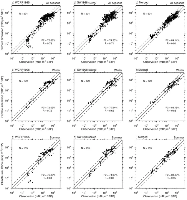
The scatter plots in Fig. 4 provide a compact overview of the model results in comparison with measurements. Each point in the figure represents one seasonal or monthly mean at one site. At the locations where measurements are available at frequencies higher than monthly, we compute the monthly mean before making the plot; at the places where only sea-sonal data are available, we simply take the seasea-sonal mean, and average the model results accordingly.
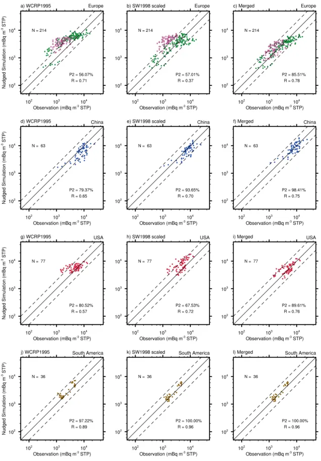
On the whole, all three simulations agree reasonably well with the observations. Taking into account all seasons and sites, more than 70 % samples are consistent with observa-tion within a factor of 2. The winter and summer results are of similar quality. The outliers in Fig. 4a and g indi-cate the underestimation of radon concentrations at Dumont d’Urville (especially in summer), which will be discussed in Sect. 3.4. Comparing the three columns in Fig. 4, one can see clearly that the merged emission map leads to bet-ter results than the other two simulations. The correlation between simulation and observation increases significantly. The overestimated concentrations in the WCRP1995 and scaled SW1998 simulations in the range between 4×10²– 6×10³mBq m−3STP are improved considerably.
To identify the reasons for the improvement, results in dif-ferent regions are shown separately in Fig. 5. In the Eu-ropean regions southward of 60◦N (excluding the Iberian Peninsula), the WCRP1995 flux of 1 atom cm−2s−1is
con-siderably stronger than the other two emission setups (cf. Fig. 2), thus in Fig. 5a the green dots reveal clear overesti-mation compared to the other two panels in the same row. Over Scandinavia the WCRP1995 and SW1998 fluxes are about 0.5 atom cm−2s−1 at most grid points, which seems still too high since almost all the pink markers in Fig. 5a and b lie outside the factor of 2 region. In contrast, the emissions derived by Szegvary et al. (2007) from the terrestrial gamma dose lead to much better results in this region (Fig. 5c).
Fig. 4.Scatter plots of the simulated and measured monthly or seasonal mean surface radon concentration (mBq m−3STP) at the 51 sites listed in Table 2 and shown in Fig. 3. The three columns correspond to simulations using the WCRP1995 recommended radon emission (left), the SW1998 emission maps scaled by a factor of 1/1.6 (middle), and the new emission maps prepared during this study. The first row contains results of all months/seasons (534 samples); The second row shows the 129 winter samples (DJF in the Northern Hemisphere, JJA in the Southern Hemisphere), and the third row shows only the 135 summer samples (JJA in the Northern Hemisphere, DJF in the Southern Hemisphere). The dashed lines indicate the range within a factor of 2 of the measurements. Also shown in each panel are the percentage of samples within this range (the P2 values) and the correlation coefficients between simulation and observation (theRvalues).
3.3 Nudged versus climatological simulations
As mentioned in the previous section, we have also per-formed simulations without nudging the model meteorol-ogy toward reanalysis. The main purpose is to evaluate the ECHAM5 model’s ability in tracer transport in a case of “free” simulation. It turns out that without nudging, the
Fig. 6.Same as Fig. 4, but for the climatological simulations without nudging.
meteorological fields. However, there is no severe deteriora-tion of the overall quality in any of the simuladeteriora-tions.
3.4 Radon concentration at individual sites
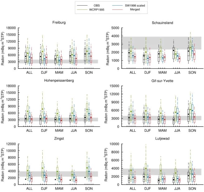
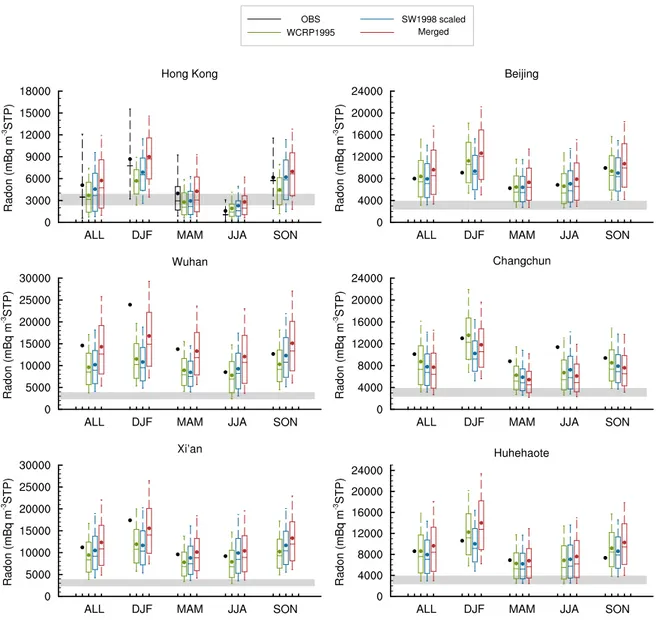
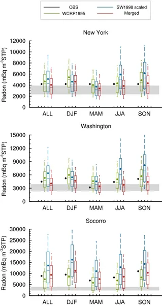
The scatter plots discussed above are derived from seasonal or monthly mean surface radon concentrations. The corre-lation between simucorre-lation and observation is mainly deter-mined by the model’s ability to reproduce the spatial distri-bution of radon concentration at regional to global scales. In this subsection we zoom in to individual sites to evaluate the simulated temporal distribution and seasonal cycle by ana-lyzing the box plots in Figs. 7–10.
Fig. 7.Box plots showing the simulated and observed distribution of surface radon concentration at six sites in Europe. The two whiskers of each box denote the 10th (lower) and 90th (upper) percentiles. Hinges from bottom to top are the 25th, 50th, and 75th percentiles, respectively. Seasonal and annual means are indicated by dots. The gray areas indicate magnitude of the equivalent radon concentration that would lead to the same ionization rate as caused by galactic cosmic rays. The lower and upper boundaries of the gray areas correspond to the 10th and 90th percentiles, respectively. See paragraph 3 of Sect. 3.4 for further details.
available. At the sites where only monthly or seasonal mean can be obtained, the seasonal mean is plotted.
Following Kazil et al. (2010) we have diagnosed in our simulations the ion production caused by galactic cosmic rays (GCR). Assuming that in the near-surface layer radon and its progeny are in equilibrium, one can easily determine (see, e.g., Laakso et al., 2004) the radon activity concentra-tion that would result in the same ionizaconcentra-tion rate (hereafter referred to as equivalent radon concentration). In Figs. 7–10, the lower and upper boundaries of the filled gray areas are the 10th and 90th percentiles of the equivalent radon con-centrations. Note that these reference percentiles are not
Fig. 8.Same as Fig. 7 but for six sites in China.
above. On the other hand, equilibrium factors between 0.5 and 0.7 are regarded as typical by Anspaugh et al. (2000) for outdoor environment, and the value 0.6 was recommended (see points 122 and 123 of Annex B therein). In other words, in a typical outdoor environment, the actual potential alpha energy concentration related to the short-lived progeny is about 50 %–70 % of the value that would prevail in the equi-librium case. Under such condition, the equivalent radon concentrations, corresponding to the cosmic ray ionisation rate, will be underestimated by (roughly) a factor of 2. One should bear this uncertainty in mind when interpreting the box plots in Figs. 7–10.
The panels in Fig. 7 confirm our findings from the scat-ter plots that over Europe, the WCRP1995 emission is on the high side, while the merged map leads to most realistic results. At Freiburg, Schauinsland, Hohenpeissenberg,
Fig. 9.Same as Fig. 7 but for three sites in the United States.
Figure 8 shows results at six Chinese sites.1 In the south-ern (e.g., Hongkong, Wuhan) and westsouth-ern (e.g., Xi’an) part of China, the simulated mean concentrations agree better with observations when the Zhuo et al. (2008) emissions are applied (see left column in Fig. 8). Note that the concen-trations are typically at the order of 5000 mBq m−3STP or higher, implying ionization rates of 3.2 pairs cm−3s−1STP or stronger. Furthermore, it is worth noting that the selected
1The measurements from Hongkong (Zahorowski et al., 2005)
were collected at Hok Tsui, an ACE-Asia (Aerosol Characteriza-tion Experiment in East Asia ) network site. Data of the five in-land cities were taken from Jin et al. (1998), each sample of which was the average of measurements collected over bare soil at several outdoor locations in the same city. The individual locations were characterized by typical regional features in terms of soil type and meteorological conditions. These measurements thus represent typ-ical radon concentrations in the corresponding regions.
cities are located in the East Asian monsoon region. The fact that the ECHAM5 model reasonably reproduces the seasonal cycle of surface radon concentration indicates that the East Asian monsoon circulation and its effect on large scale tracer transport is well represented by the model.
From Fig. 9 we see again that the SW1998 emission, even though scaled down by a factor of 1.6, is too high in the USA. The inter-city differences suggest that taking into account the regional gradient in radon flux improves the results in gen-eral.
In Fig. 10, results are presented for eight coastal and re-mote ocean sites. Bermuda and Mauna Loa are typical exam-ples of remote ocean sites, while Cape Grim and Cape Point are coastal sites, all strongly affected by horizontal transport. At these sites the model is able to reproduce not only the cor-rect magnitude and seasonal cycle of the population mean, but also the characteristic shapes of the concentration distri-bution. The strongly asymmetric distributions at Cape Grim and Cape Point are well captured. This indicates that both the variations in large scale circulation and the radon emission in source regions are reasonably represented in the model.
Kerguelen and Crozet are also remote ocean sites, but fea-ture extremely low radon concentration because of their lo-cation in the Southern Ocean. At these two sites we again see a strong sensitivity to emission. Over the ocean, both the WCRP1995 recommendation and the modified SW1998 map have zero radon flux, while the merged emission map utilizes the space- and time-dependent estimates of Schery and Huang (2004). In the storm track over the Southern Ocean, the surface radon flux are relatively large due to strong surface winds. In the region 40◦S–60◦S, 0◦E–180◦, the annual mean exceeds 0.005 atom cm−2s−1(cf. Fig. 1 in Schery and Huang, 2004). Although the flux is very weak compared to that over the continents, taking it into account does improve the results over the remote oceans significantly (Fig. 10, row 3).
Fig. 10.Same as Fig. 7 but for coastal and oceanic sites. Most panels in this figure do not have a gray box in them because at these sites the radon family induces much less ionizing energy than the cosmic rays. The gray box is therefore literally off the chart.
over Antarctica to zero. Compared to WCRP1995, this sim-ulation has non-zero fluxes over the Southern Oceans (Sch-ery and Huang, 2004), which, through transport, can affect Antarctica. It turns out that the concentrations at Dumont d’Urville and Mawson become slightly higher than in the WCRP1995 simulation (not shown), but there is no essen-tial improvement either in the magnitude of the concentra-tion or in its seasonal cycle. This indicates that (at least in
Fig. 11.Simulated annual and seasonal mean near-surface ionization rate induced by radon decay series (IPRR, unit: cm−3s−1).
3.5 A brief summary on model evaluation
From the analysis presented in this section, we see that the ECHAM5 model performs reasonably well in simulating the lifecycle and global distribution of radon. Using the most up-to-date emission estimates, we are able to reproduce the main features of the temporal and spatial distribution of the surface radon concentration. At most of the sites shown in Fig. 3, model results agree not only qualitatively but also quantitatively well with measurements. On the one hand, there is still quite some room for improvement, for exam-ple, by compiling even more detailed and accurate emission maps, and by enhancing the model resolution so as to bet-ter resolve the atmospheric circulation and surface properties at scales smaller than 200 km; On the other hand, the sim-ulations shown here are reasonable, and compare well with other models (see, e.g., Dentener et al., 1999; Taguchi et al., 2002; Hauglustaine et al., 2004; Koch et al., 2006, among others). This provides a solid base for estimating the radon-related ionization rate.
4 Radon-related ionization
In this section we present the simulated ionization rate caused by radon and its progeny. In the simplified decay chain (Fig. 1b) there are three sources of ionizing radia-tion: the decay of222Rn, 214Pb and214Bi. Since the life-times of the two daughters are relatively short compared to the model time step (12 min), their concentrations are not strongly affected by transport, but rather determined by how much radon is locally availably for radioactive decay. Thus the global distribution of the resulting ionization closely re-sembles that of radon concentration (not shown). For brevity, in the following we will refer to the radon-related ionization rate (i.e., variableψin Eqn. 1) as IPRR.
4.1 Global distribution
Fig. 12. Left column: simulated zonal mean ionization rate over the continents caused by the radioactive decay of radon and its progeny (IPRR, unit: cm−3s−1); Middle column: as in the left column but caused by galactic cosmic rays (IPRC, unit: cm−3s−1); Right column: the contribution of radon and its progeny to the total (IPRR+IPRC) ionization rate. All panels correspond to the simulation performed with the merged emission map.
stability leads to high IPRR over 9 cm−3s−1 (Fig. 11d–f). The summer ionization rates are considerably lower due to the ventilation effect of convective transport (Fig. 11g–i).
Discrepancies among the three columns in Fig. 11 indicate the impact of radon emission. The scaled SW1998 map leads to stronger ionization over West US and Europe than in the other two simulations, while in China the IPRR is highest when the Zhuo et al. (2008) emission is applied (Fig. 11c, f, i). These are all consistent with what we have seen in Fig. 2. Considering the model evaluation results in Sect. 3, the IPRR given by the merged emission map is probably the most ac-curate in the above-mentioned regions. It is worth noting that panels d–f of Fig. 11 reveal large discrepancies over Russia as well. There the SW1998 emission map gives the high-est IPRR among the three simulations (Fig. 11e), while the Szegvary et al. (2007) emission corresponds to the lowest values (Fig. 11f). Due to lack of long-term observation, we are not yet able to judge the quality of the simulations in this area. Nevertheless differences between the two panels are still informative because they provide an (although far from conclusive) estimate about the uncertainty of the IPRR in this area.
It would be useful if we could compare the simulated radon-induced ionization rate with some direct ionization rate measurements (e.g, Gagn´e et al., 2010). However,
un-like the radon concentration, the ionization rate induced by the radon family can not be directly measured but has to be derived. One way is to subtract the external ionization from the observed total amount and attribute the residual to the radon family, assuming that there is no other radionuclide in the air. The second and often used method is to compute the radon-induced ionization rate from the activity concen-trations of radon and its progeny. The problem here is that not all the daughters can be directly measured. Before com-puting the ionization rate, one has to first derive the activity concentration of these unmeasurable daughters by assuming a certain equilibrium factor (Anspaugh et al., 2000) for the decay chain. Both of the two methods need additional in-formation of other ionization agents and assumptions made would bring additional uncertainty. Therefore, we are not able to get accurate measurements of radon-induced ioniza-tion rate and use them to evaluate the model directly.
Fig. 13. Height-longitude cross section of the 20◦N–50◦N mean ionization rate over land caused by radon and its progeny. The re-sults are obtained using the newly merged radon emission map.
its magnitude clearly exceeds the GCR-induced ionization (Fig. 12, right most column). It should be noted that in bo-real winter, very high ionization rates appear between 20◦N and 50◦N (Fig. 12d). The major contributor to these maxima in the zonal mean is the high IPRR in Asia (China, Myanmar, and north of India) and the US, as can be seen from the east-west cross section in Fig. 13. These regions are known to be associated with relative high near-surface SO2 and H2SO4
concentrations as well as nucleation rates (see, e.g., Figs. 1– 2 in Yu et al. (2008)), especially in cold seasons when SO2
emissions are strong and the stable atmospheric boundary layer traps the species in the surface layer. Under such condi-tions, the coexistence of high ionization rate may help further enhance the particle formation prcesses.
4.2 Ionization rate and ambient temperature
Temperature and H2SO4 concentration are generally
be-lieved as the two most important factors controlling the start and end of nucleation events (see, e.g, Yu, 2010). In this sub-section we intend to look into the coexistence of ionization with these parameters. Due to the fact that we did not switch
on aerosol and chemistry processes in the simulations, con-centrations of H2SO4are not available. Thus only the
ambi-ent temperature is analyzed here.
Figure 14 shows the joint probability density distribution (PDF) of air temperature and radon-related ionization rate in different regions (China, Europe, North America, and Rus-sia, as indicated in Fig. 11e–f by dashed black lines). The PDFs are computed for the lowest model level using the 3-hourly data in winter (DJF). According to the evaluations in the previous section, the simulation using the merged radon emission is the most accurate in China, Europe, and North America. Therefore only this simulation is shown for these regions (Fig. 14a–c).
The most prominent feature in the first row of Fig. 14 is that ionization is much stronger over China and asso-ciated with lower temperature. The PDF of temperature peaks around 260 K. At this temperature, ionization rate of 15 cm−3s−1is not at all uncommon (Fig. 14a). In extreme cases, the ionization rate can even reach 50 cm−3s−1at tem-peratures as low as 250 K (not shown). If there is abundant sulfuric acid gas, charged H2SO4/H2O nucleation may be
strong and significantly influence the aerosol size distribu-tion. In the US, ionization is also strong, and peaks around 0◦C (Fig. 14b). Europe, on the other hand, features very low ionization rate which probably has very limited influence on nucleation. The second row of Fig. 14 shows the joint PDF in Russia for all three simulations since it is not clear which one is more accurate. Although the simulated ionization rates are lower than in China and the US, the effect of low temperature may play a role and still leads to significant particle forma-tion if other condiforma-tions of nucleaforma-tion are fulfilled.
It should be pointed out that with Fig. 14 we only pre-sented a very preliminary analysis showing that radon-related ionization may play a significant role in new particle forma-tion at particular locaforma-tions. In order to obtain more concrete results on the actual impact of such ionization, one should actually include the radon-related ionization in an aerosol-climate model and carry out sensitivity studies, because in re-ality the nucleation processes are highly complex and nonlin-ear, and not yet well understood. For example, in this section we analyzed only boreal winter although nucleation events are often observed to peak in spring and fall (e.g., Laakso-nen et al., 2008). It would be interesting to carry out simula-tions with the ECHAM5-HAM model (Stier et al., 2005) to find out whether the radon-family plays a role (at least in this particular model) in the phenomena.
5 Conclusions
Fig. 14. Joint (bivariate) probability density distribution (PDF) of air temperature and radon-related ionization rate (IPRR) in different regions: (a)China (20◦N–50◦N, 75◦E–120◦E);(b)Europe (40◦N–75◦N, 10◦W–40◦E);(c)USA (30◦N–50◦N, 120◦W–70◦W);(d– f)Russia (50◦N–80◦N, 40◦E–180◦E). These regions are indicated by dashed black frames in Fig. 11. Labels next to the color bar are intensities of the PDF (unit: %). The PDFs are computed for the near-surface from the 3-hourly model output in winter months (DJF). Marginal area with white color indicate missing values. Note that scales of the temperature coordinate in(a–c)are not the same as those in (d–f).
computed analytically within each model time step, and cou-pled with tracer transport caused by advection, cumulus con-vection and turbulent mixing. The radon-related ionization rate is estimated based on the activity concentration of radon and its daughter species, and well-accepted values of the de-cay/ionization energy.
Based on recent reports in the literature on radon emission, an up-to-date global radon emission map is compiled with regional details and seasonal variation. The simulated radon activity concentration is evaluated against surface radon mea-surements at 51 locations. Results show that the global model ECHAM5 can reasonably reproduce the variations of surface radon concentrations observed at various locations. On the whole, the newly compiled emission map leads to better results compared to the WCRP1995 protocol and the widely used SW1998 map. The merged map is not only helpful for this study, but probably also useful for other re-searchers working on numerical modelling of radon trans-port and the transtrans-port and deposition processes of210Pb (e.g., Balkanski et al., 1993).
The radon-related ionization rate is computed and com-pared with the GCR-ionization rate. It is found that in bo-real winter, the suppressed vertical transport due to increased
atmospheric stability leads to seasonal mean IPRR as high as 9 cm−3s−1. In middle- and low-latitude continental areas, the zonal mean radon-induced ionization rate clearly exceeds the GCR-induced counterpart in the near-surface levels up to 800 m elevation. At many continental sites, the observed and simulated surface radon activity concentration often occurs well above the 90th percentile of the equivalent concentra-tion derived from the GCR-induced ionizaconcentra-tion. Further anal-ysis on the joint PDF of ionization rate and temperature show that in China and USA, strong radon-related ionization of-ten occur in winter at low ambient temperature, which may help enhance the H2SO4/H2O nucleation when other factors
such as H2SO4 concentration and relative humidity are in
favorable conditions. Based on results from this study we conclude that it will be useful to extend the work of Kazil et al. (2010) and carry out a follow-up study with the aerosol-climate model ECHAM5-HAM to investigate the effect of radon-related ionization on nucleation, as well as the con-sequences in aerosol size distribution, cloud properties, and climate effect.
from the journal website. Ionization rates at higher temporal resolution, as well as the merged radon emission maps, can be provided to interested researchers upon request.
Appendix A
Analytical solution of the decay chain
The simplified decay chain system (Fig. 1b) can be described by an ordinary differential equation system with four un-knowns (in activity concentration form):
dc1
dt = −λ1c1, (A1)
dc2 dt =
λ1
λ2c1−λ2c2, (A2)
dc3 dt =
λ2 λ3
c2−λ3c3, (A3)
dc4 dt =
λ3
λ4c3, (A4)
where c1, c2, c3, and c4 are the activity concentration of 222Rn, 214Pb, 214Bi, and 210Pb, respectively, and λ
1, λ2, λ3, andλ4are the corresponding decay constants. For each
model time step (1t=12 min), the analytical solution of the decay chain att+1t reads
c1(t+1t )=c1(t )e−λ11t, (A5) c2(t+1t )=c2(t )e−λ21t+χ21η12c1(t ), (A6) c3(t+1t )=c3(t )e−λ31t+χ21χ31η13c1(t )
+χ32η23(c2(t )−χ21c1(t )) (A7)
where χij =
λi λi−λj
, (A8)
ηij =e−λi1t−e−λj1t. (A9)
By integrating Eqs. (A5)–(A7) fromttot+1t, the time-step average concentration can be obtained:
¯
c1=θ1c1(t ), (A10)
¯
c2=θ2c2(t )+χ21(θ1−θ2)c1(t ), (A11) ¯
c3=θ3c3(t )+χ21χ31(θ1−θ3)c1(t )
+χ32(θ2−θ3)(c2(t )−χ21c1(t )). (A12)
where θi=
λi−e−λi1t λi1t
. (A13)
Since the decay of210Pb is ignored, its concentration is not computed in the model.
Supplement related to this article is available online at: http://www.atmos-chem-phys.net/11/7817/2011/ acp-11-7817-2011-supplement.pdf.
Acknowledgements. The authors thank F. Conen and T. Szegvary for providing their radon flux maps, and S. Rast for preparing the nudging data and making the internal review. We are also grateful to S. Schery, S. Whittlestone, C. Schlosser, J.-F. Vinuesa, and the two anonymous reviewers for their very helpful comments. The German BfS, French RAMCES, and Australian ANSTO monitoring networks are acknowledged for providing the new radon measurements used in this study. This work was jointly supported by the Max Planck Society and the EUCAARI project. All simulations were performed at the German Climate Computing Center (Deutsches Klimarechenzentrum GmbH, DKRZ).
The service charges for this open access publication have been covered by the Max Planck Society.
Edited by: M. Schulz
References
Anspaugh, L., Bennett, B., Bouville, A., Burkart, W., Cox, R., Croft, J., Hall, P., Leenhouts, H., Muirhead, C., Ron, E., Savkin, M., Shrimpton, P., Stather, J., Thacker, J., and Wrixon, A.: Exposures from natural radiation sources, ANNEX B of Sources and effects of ionizing radiation, UNSCEAR 2000 Report to the General Assembly, Tech. Rep. E.00.IX.3, United Nations Scientific Committee on the Effects of Atomic Radia-tion, New York, USA, 2000.
Bakwin, P. S., Zhao, C., Ussler, W., Tans, P. P., and Quesnell, E.: Measurements of carbon dioxide on a very tall tower, Tellus B, 47, 535–549, 1995.
Balkanski, Y. J., Jacob, D. J., Gardner, G. M., Graustein, W. C., and Turekian, K. K.: Transport and residence times of tropospheric aerosols inferred from a global three-dimensional simulation of Pb., J. Geophys. Res., 98, 20573–20586, 1993.
Brinkop, S. and Roeckner, E.: Sensitivity of a general circula-tionmodel to parameterizations of cloud-turbulence interactions inthe atmospheric boundary layer, Tellus A, 47, 197–220, 1995. Brunke, E. G., Labuschagne, C., Parker, B., Scheel, H. E., and
Whit-tlestone, S.: Baseline air mass selection at Cape Point, South Africa: application of222Rn and other filter criteria to CO2, At-mos. Environ., 38, 5693–5702, 2004.
Chevillard, A., Ciais, P., Karstens, U., Heimann, M., and Schmidt, M.: Transport of 222Rn using the regional model REMO: a detailed comparison with measurements over Europe, Tellus B, 54, 850–871, 2002.
Clement, C. F. and Harrison, R. G.: The charging of radioactive aerosols, J. Aerosol Sci., 23, 481–504, 1992.
Conen, F. and Robertson, L. B.: Latitudinal distribution of radon-222 flux from continents, Tellus B, 54, 127–133, 2002.
Dentener, F., Feichter, J., and Jeuken, A.: Simulation of222Radon using on-line and off-line global models, Tellus B, 51, 573–602, 1999.
Downey, A., Jasper, J. D., Gras, J. J., and Whittlestone, S.: Lower tropospheric transport over the Southern Ocean, J. Atmos. Chem., 11, 43–68, 1990.
Emsley, J.: Nature’s building blocks: an A–Z guide to the elements, Oxford University Press Inc., New York, USA, 354–355, 2001. Gagn´e, S., Nieminen, T., Kurt´en, T., Manninen, H. E., Pet¨aj¨a, T.,
Laakso, L., Kerminen, V.-M., Boy, M., Kulmala, M.: Fac-tors influencing the contribution of ion-induced nucleation in a boreal forest, Finland, Atmos. Chem. Phys., 10, 3743–3757, doi:10.5194/acp-10-3743-2010, 2010.
Gold, S., Barkhau, H. W., Shleien, B., and Kahn, B.: Measurement of naturally occurring radionuclides in air, University of Chicago Press, Chicago, United States, 1964.
Goto, M., Moriizumi, J., Yamazawa, H., Iida, T., and Zhuo, W.: Es-timation of global radon exhalation rate distribution, AIP Conf. Proc., 1034, 169–172, 2008.
Griffiths, A. D., Zahorowski, W., Element, A., and Werczynski, S.: A map of radon flux at the Australian land surface, Atmos. Chem. Phys., 10, 8969–8982, doi:10.5194/acp-10-8969-2010, 2010. Guelle, W., Balkanski, Y. J., Schulz, M., Dulac, F., and Monfray, P.:
Wet deposition in a global size-dependent aerosol transport model 1. Comparison of a 1 year210Pb simulation with ground measurements, J. Geophys. Res., 103(D10), 11429–11445, 1998. Harrison, R. G. and Carslaw, K. S.: Ion-aerosol-cloud pro-cesses in the lower atmosphere, Rev. Geophys., 41, 1012, doi:10.1029/2002RG000114, 2003.
Hatakka, J., Aalto, T., Aaltonen, V., and Aurela, M.: Overview of the atmospheric research activities and results at Pallas GAW sta-tion, Boreal Environ. Res., 8, 365–383, 2003.
Hauglustaine, D. A., Hourdin, F., Jourdain, L., Filiberti, M. A., Walters, S., Lamarque, J. F., and Holland, E. A.: Interac-tive chemistry in the laboratoire de meteorologie dynamique general circulation model, J. Geophys. Res., 109, D04314, doi:10.1029/2003JD003957, 2004.
Heimann, M., Monfray, P., and Polian, G.: Modeling the long-range transport of222Rn to subantarctic and arctic areas, Tellus B, 42, 83–99, 1990.
Hirao, S., Nono, Y., Yamazawa, H., Moriizumi, J., Iida, T., and Yoshioka, K.: Development and verification of long-range at-mospheric transport model of radon-222 and lead-210 includ-ing scavenginclud-ing process, in: The Natural Radiation Environment, edited by: Paschoa, A. S. and Steinh¨ausler, F., vol. 1034, Ameri-can Institute of Physics, Buzios, Brazil, 407–410, 2008. Hosler, C. R.: Urban-rural climatology of atmospheric radon
con-centration, J. Geophys. Res., 73, 1155–1166, 1968.
Hutter, A. R., Larsen, R. J., Maring, H., and Merrill, J. T.: 222Rn at Bermuda and Mauna Loa: local and distant sources, J. Ra-dioanal. Nucl. Ch., 193, 309–318, 1995.
Jacob, D. J. and Prather, M. J.: Radon-222 as a test of convective transport in a general circulation model, Tellus B, 42, 118–134, 1990.
Jacob, D. J., Prather, M. J., Rasch, P. J., Shia, R.-L., Balkanski, Y. J., Beagley, S. R., Bergmann, D. J., Blackshear, W. T., Brown, M., Chiba, M., Chipperfield, M. P., Grandpr´e, J., Dignon, J. E., Fe-ichter, J., Genthon, C., Grose, W. L., Kasibhatla, P. S., K¨ohler, I., Kritz, M. A., Law, K., Penner, J. E., Ramonet, M., Reeves, C. E., Rotman, D. A., Stockwell, D. Z., Van Velthoven, P., Verver, G., Wild, O., Yang, H., and Zimmermann, P.: Evaluation and inter-comparison of global atmospheric transport models using222Rn and other short-lived tracers, J. Geophys. Res., 102, 5953–5970, 1997.
Jesse, W. P.: Precision measurements ofWfor polonium alpha
par-ticles in various gases, Radiat. Res., 33, 229–237, 1968. Jeuken, A., Siegmund, P., Heijboer, L., Feichter, J., and
Bengts-son, L.: On the potential of assimilating meteorological analyses in a global climate model for the purposes of model validation, J. Geophys. Res., 101, 16939–16950, 1996.
Jin, Y., Iida, T., Wang, Z., Ikebe, Y., and Abe, S.: A subnationwide survey of outdoor and indoor222Rn concentrations in China by passive method. Radon and thoron in the human environment, in: Radon and Thorn in the Human Environment, in: Proceedings of the 7th Tohwa University International Symposium, edited by: Katase, A. and Shimo, M., World Scientific Publishing Co. Pre. Ltd., Singapore, 276–281, 1998.
Josse, B., Simon, P., and Peuch, V. H.: Radon global simulations with the multiscale chemistry and transport model MOCAGE., Tellus B, 56, 339–356, 2004.
Kazil, J., Lovejoy, E. R., Barth, M. C., and O’Brien, K.: Aerosol nucleation over oceans and the role of galactic cosmic rays, At-mos. Chem. Phys., 6, 4905–4924, doi:10.5194/acp-6-4905-2006, 2006.
Kazil, J., Stier, P., Zhang, K., Quaas, J., Kinne, S., O’Donnell, D., Rast, S., Esch, M., Ferrachat, S., Lohmann, U., and Feichter, J.: Aerosol nucleation and its role for clouds and Earth’s ra-diative forcing in the aerosol-climate model ECHAM5-HAM, Atmos. Chem. Phys., 10, 10733–10752, doi:10.5194/acp-10-10733-2010, 2010.
Koch, D., Schmidt, G. A., and Field, C. V.: Sulfur, sea salt and radionuclide aerosols in GISS ModelE, J. Geophys. Res., 111, D06206, doi:10.1029/2004JD005550, 2006.
Kulmala, M., Vehkam¨aki, H., Pet¨aj¨a, T., Dal Maso, M., Lauri, A., Kerminen, V.-M., Birmili, W., and McMurry, P. H.: Formation and growth rates of ultrafine atmospheric particles: a review of observations, J. Aerosol Sci., 35, 143–176, 2004.
Laakso, L., Pet¨aj¨a, T., Lehtinen, K. E. J., Kulmala, M., Paatero, J., H¨orrak, U., Tammet, H., and Joutsensaari, J.: Ion production rate in a boreal forest based on ion, particle and radiation measure-ments, Atmos. Chem. Phys., 4, 1933–1943, doi:10.5194/acp-4-1933-2004, 2004.
Laaksonen, A., Kulmala, M., O’Dowd, C. D., Joutsensaari, J., Vaat-tovaara, P., Mikkonen, S., Lehtinen, K. E. J., Sogacheva, L., Dal Maso, M., Aalto, P., Petaja, T., Sogachev, A., Yoon, Y. J., Lihavainen, H., Nilsson, D., Facchini, M. C., Cavalli, F., Fuzzi, S., Hoffmann, T., Arnold, F., Hanke, M., Sellegri, K., Umann, B., Junkermann, W., Coe, H., Allan, J. D., Al-farra, M. R., Worsnop, D. R., Riekkola, M.-L., Hyotylainen, T., and Viisanen, Y.: The role of VOC oxidation products in con-tinental new particle formation, Atmos. Chem. Phys., 8, 2657– 2665, doi:10.5194/acp-8-2657-2008, 2008.
van der Laan, S., Neubert, R. E. M., and Meijer, H. A. J.: Methane and nitrous oxide emissions in The Netherlands: ambient mea-surements support the national inventories, Atmos. Chem. Phys., 9, 9369–9379, doi:10.5194/acp-9-9369-2009, 2009.
Lambert, G., Polian, G., Sanak, J., Ardouin, B., Buisson, A., Je-gou, A., and Le Roulley, J. C.: Cycle du radon et de ses descendants: application `a l’´etude des ´echanges troposph`ere-stratosph`ere, Ann. Geophys., 38, 497–531, 1982,
http://www.ann-geophys.net/38/497/1982/.
Res., 54, 23252–23270, 1995.
Levin, I., Born, M., Cuntz, M., Langendorfer, U., Mantsch, S., Naegler, T., Schmidt, M., Varlagin, A., Verclas, S., and Wagen-bach, D.: Observations of atmospheric variability and soil exha-lation rate of radon-222 at a Russian forest site. Technical ap-proach and deployment for boundary layer studies, Tellus B, 54, 462–475, 2002.
Lin, S. J. and Rood, R. B.: Multidimensional flux-form semi-Lagrangian transport schemes, Mon. Weather Rev., 124, 2046– 2070, 1996.
Lindeken, C. L.: Seasonal variations in the concentration of air-borne radon and thoron daughters, Tech. Rep. USAEC Rep. UCRL-50007, University of California Lawrence Radiation Lab-oratory, Livermore, CA, USA, 1966.
Lockhart, L. B.: Atmospheric radioactivity in South America and Antarctica, J. Geophys. Res., 65, 3999–4005, 1960.
Lockhart, L. B.: Radioactivity of the radon-222 and radon-220 se-ries in the air at ground level, in: The Natural Radiation Environ-ment, edited by: Adams, J. A. and Lowder, W. M., University of Chicago Press, Chicago, USA, 331–344, 1964.
Lockhart, L. B., Patterson, R. L., and Saunders, A. W.: Airborne ra-dioactivity in Antarctica, J. Geophys. Res., 71, 1985–1991, 1966. Louis, J. F.: A parametric model of vertical eddy uses in the
atmo-sphere, Bound.-Lay. Meteorol., 17, 187–202, 1979.
Lovejoy, E. R., Curtius, J., and Froyd, K. D.: Atmospheric ion-induced nucleation of sulfuric acid and water, J. Geophys. Res., 109, D08204, doi:10.1029/2003JD004460, 2004.
Lupu, A. and Cuculeanu, V.: Vertical distribution of radon progeny over vegetated ground, J. Geophys. Res., 104, 27527–27533, 1999.
Martens, C. S., Shay, T. J., Mendlovitz, H. P., Matross, D. M., Saleska, S. R., Wofsy, S. C., Stephen Woodward, W., Men-ton, M. C., De Moura, J. M. S., Crill, P. M., De Moraes, O. L. L., and Lima, R. L.: Radon fluxes in tropical forest ecosystems of Brazilian Amazonia: night-time CO2 net ecosystem exchange derived from radon and eddy covariance methods., Global Change Biol., 10, 618–629, 2004.
Mattsson, R.: Seasonal variation of short-lived radon progeny, Pb210 and Po210, in ground level air in Finland, J. Geophys. Res., 75, 1741–1744, 1970.
Mishra, U. C., Rangarajan, C., and Eapen, C. D.: Natural radioac-tivity of the atmosphere over the Indian land mass, inside deep mines, and over adjoining oceans, US Department of Energy, Washington, DC, USA, 327–346, 1980.
Nagaraja, K., Prasad, B. S. N., Madhava, M. S., Chan-drashekara, M. S., Paramesh, L., Sannappa, J., Pawar, S. D., Mu-rugavel, P., and Kamra, A. K.: Radon and its short-lived progeny: variations near the ground, Radiat. Meas., 36, 413–417, 2003. Nordeng, T. E.: Extended versions of the convective
parametriza-tion scheme at ECMWF and their impact on the mean and tran-sient activity of the model in the tropics, ECMWF Research Department, Technical Momorandum 206, European Centre for Medium-Range Weather Forecast, Reading, UK, 1994. Papastefanou, C.: Radioactive Aerosols, Elsevier, Amsterdam, The
Netherlands, 16–17, 2008.
Polian, G., Lambert, G., Ardouin, B., and Jegou, A.: Long-range transport of continental radon in sub-Antarctic and Antarctic ar-eas, Tellus B, 38, 178–189, 1986.
Porstend¨orfer, J.: Properties and behaviour of radon and thoron and
their decay products in the air, J. Aerosol Sci., 25, 219–263, 1994.
Ramamurthi, M., Strydom, R., Hopke, P. K., and Holub, R. F.: Nanometer and ultrafine aerosols from radon radiolysis, J. Aerosol Sci., 24, 393–407, 1993.
Ramonet, M., Schmidt, M., P´epin, L., Kazan, V., Picard, D., Fil-ippi, D., Jourd’heuil, L., Valant, C., Monvoisin, G., Sarda, R., and Ciais, R.: The French Trace Gas Monitoring Program RAMCES, in: Report of the Eleventh WMO/IAEA Meeting of Experts on Carbon Dioxide Concentration and Related Tracer Measurement Techniques, edited by: Toru, S. and Kazuto, S., WMO/GAW Re-port 148, Tokyo, Japan, 136–148, 2003.
Rasch, P. J., Feichter, J., Law, K., Mahowald, N., Pen-ner, J., Benkovitz, C., Genthon, C., Giannakopoulos, C., Ka-sibhatla, P., Koch, D., Levy, H., Maki, T., Prather, M., Roberts, D. L., Roelofs, G.-J., Stevenson, D., Stockwell, Z., Taguchi, S., Kritz, M., Chipperfield, M., Baldocchi, D., Mc-Murry, P., Barrie, L., Balkanski, Y., Chatfield, R., Kjell-strom, E., Lawrence, M., Lee, H. N., Lelieveld, J., Noone, K. J., Seinfeld, J., Stenchikov, G., Schwartz, S., Walcek, C., and Williamson, D.: A comparison of scavenging and deposition processes in global models: results from the WCRP Cambridge Workshop of 1995, Tellus B, 52, 1025–1056, 2000.
Robertson, L. B., Stevenson, D. S., and Conen, F.: Test of a northwards-decreasing 222Rn source term by comparison of modelled and observed atmospheric222Rn concentrations, Tel-lus B, 57, 116–123, 2005.
Roeckner, E., B¨auml, G., Bonaventura, L., Brokopf, R., Esch, M., Giorgetta, M., Hagemann, S., Kirchner, I., Kornblueh, L., Manzini, E., Rhodin, A., Schlese, U., Schulzweida, U., and Tompkins, A.: The atmospheric general circulation model ECHAM 5. PART I: model description, MPI Technical Report 349, Max Planck Institute for Meteorology, Hamburg, Germany, 2003.
Ross, J. O.: Simulation of atmospheric krypton-85 transport to as-sess the detectability of clandestine nuclear reprocessing, Re-ports on Earth System Science 82, Max Planck Institute for Me-teorology, Hamburg, 2010.
Schery, D.: Progress on Global222Rn Flux Maps and Recommen-dations for Future Research, in: 1st International Expert Meeting on Sources and Measurements of Natural Radionuclides Applied to Climate and Air Quality Studies (Gif-sur-Yvette, France, June 2003), edited by: Barrie, L. A. and Lee, H. N., WMO TD 1201, Gif-sur-Yvette, France, 43–47, 2004.
Schery, S. D. and Huang, S.: An estimate of the global distribu-tion of radon emissions from the ocean, Geophys. Res. Lett., 31, L19104, doi:10.1029/2004GL021051, 2004.
Schery, S. D. and Wasiolek, M. A.: Modeling radon flux from the Earth’s surface, in: Radon and Thorn in the Human Environment, in: Proceedings of the 7th Tohwa University International Sym-posium, edited by: Katase, A. and Shimo, M., World Scientific Publishing Co. Pre. Ltd., Singapore, 73–78, 1998.
Servant, J. and Tanaevsky, O.: Mesures de la radioactivite naturelle dans la region Parisienne, Ann. Geophys., 17, 405–409, 1961, http://www.ann-geophys.net/17/405/1961/.