Property Rights as a Public Policy Tool: An
Empirical Analysis of the Social and Economic
E¤ects
Mauricio José Serpa Barros de Moura
Contents
Contents 1
List of Tables 3
List of Figures 4
1 Introduction 1
2 The Data 7
2.1 Minimizing Endogeneity Bias Concerns . . . 9
3 Econometric Model: Di¤erence-in-Di¤erence Estimates 12
3.1 Di¤erence-in-Di¤erence Estimates: Estimator – General Framework . 12
3.2 Di¤erence-in-Di¤erence Estimates: The Basic Regression Model . . . 15
4 How Does Land Title A¤ect Income and Labor Supply? 16
4.1 Basic Findings - Hours Worked and Income . . . 16
4.2 Di¤erence-in-Di¤erence Estimates: Land Title Speci…cation . 20
4.3 Results . . . 22
4.4 Labor Supply of Low Income Households . . . 25
4.6 Results . . . 30
5 How Does Land Title A¤ect Child Labor? 34 5.1 Child Labor Force Participation: The Economic Context . . . 34
5.2 Basic Findings – Child Labor Force . . . 37
5.3 Di¤erence-in-Di¤erence Estimates: Land Title Speci…caton . . . 40
5.4 Results . . . 42
6 How Does Land Title Improve Happiness? 45 6.1 Happiness in Economics: Theory and Data . . . 45
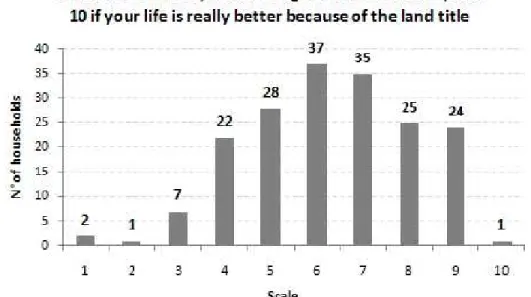
6.2 Basic Statistics – Happiness and Land Title . . . 48
6.3 The Multinomial Probit Model . . . 52
6.3.1 Predicted Probabilities . . . 55
6.3.2 Partial E¤ects of Continuous Covariates . . . 56
6.3.3 Partial E¤ects of Discrete Covariates . . . 57
6.4 Multinomial Probit Model: Land Title Speci…cation for Happiness . . 57
6.5 Results . . . 59
6.5.1 Predicted Probabilities – The Partial E¤ects of Land Title . . 61
7 Conclusion 63
8 Appendix A: Complete Stage I and Stage II Questionnaires 74
9 Appendix B: Microeconomic Framework 98
9.1 Microeconomic Framework - The Basics . . . 98
9.2 Microeconomic Framework - Labor Supply of Children . . . 102
10 Appendix C: Basic Statistics 104
11 Appendix D: 112
12 Appendix E: Osasco’s Map 116
13 Appendix F: Google Earth’s Pictures 117
14 Appendix G: Pictures from DR 119
15 Appendix H: Income x Land Title Diagrams 121
16 Appendix I: Child Labor x Land Title Diagrams 131
17 Appendix J: Intercept in Ordered Probit Models 134
List of Tables
1 Income Card . . . 18
3 Intensive Labor Force: Working 2007 2008 . . . 23
4 Income Regression . . . 24
5 Quantiles of income (Minimum Wages) in 2007 for complete sample . 25 6 Estimates of impact of property rights on labor supply . . . 30
7 Robustness Check without Income . . . 31
8 Labor Intensive Quantile Regression (without income) . . . 33
9 Sample means - with all households that have children . . . 43
10 Child Labor and Land Title . . . 44
11 Happiness and Land Title . . . 60
12 Predicted Probabilities . . . 62
13 Sample means - with all households that have not moved . . . 112
14 Sample Means - Households that not moved . . . 113
15 Sample Means - Households that moved . . . 114
16 Tests of means for covariates in 2007 . . . 115
List of Figures
1 Land Registration . . . 22 How land title a¤ected household’s life? . . . 6
4 Level of Income (Minimum Wage) x Number of Households . . . 19
5 Intensive Labor Force: Working 2007 2008 . . . 20
6 Occupation level among the 5-17 year-old population (Percentual of
total 5-17 population) . . . 35
7 Are there any child/teenager helping in family income? How many? . 38
8 Child Labor Force Hours Worked Weekly x Number of Households
(Sample) . . . 39
9 Child Labor Force Hours Worked Weekly x Number of Households
(Control Group) . . . 40
10 Taken all together, how would you say things are these days - would
you say that you are...? . . . 49
11 Taken all together, how would you say things are these days - would
you say that you are...? . . . 50
12 On the whole, about the life that you lead, are you...? . . . 51
13 On the whole, about the life that you lead, are you...? . . . 52
14 Comparing distributions of "weekly hours of adult work" for treated
and control on the average income distribution in 2007 . . . 104
15 Comparing distributions of "weekly hours of adult work" for treated
16 Comparing distributions of "weekly hours of adult work" for treated
and control on the lower quartile of income distribution in 2007 . . . 106
17 Comparing distributions of "weekly hours of adult work" for treated and control on the average income distribution in 2008 . . . 107
18 Comparing distributions of "weekly hours of adult work" for treated and control on the lower quartile of income distribution in 2008 . . . 108
19 Comparing distributions of "weekly hours of adult work" for treated and control on the upper quartile of income distribution in 2008 . . . 109
20 Hours Worked Weekly x Number of Households: Households that not moved - Sample . . . 110
21 Number of Minimum Wage x Number of Households: Households that not moved - Sample . . . 111
22 Osasco’s Map . . . 116
23 Jardim Canaã . . . 117
24 Jardim DR I . . . 118
25 Jardim DR II . . . 119
26 Jardim DR III . . . 120
27 Selected Variables by Land Title: Age . . . 121
29 Selected Variables by Land Title: Employed . . . 123
30 Selected Variables by Land Title: Hours Worked Weekly . . . 124
31 Selected Variables by Land Title: Increase in Hours Worked . . . 125
32 Selected Variables by Land Title: Income . . . 126
33 Selected Variables by Land Title: Increase in Income . . . 127
34 Selected Variables by Land Title: Increase in Income by Gender . . . 128
35 Selected Variables by Land Title: Increase in Income by Race . . . . 129
36 Selected Variables by Land Title: Time in Residency . . . 130
37 Selected Variables by Land Title . . . 131
38 Histogram Works Worked Weekly by Adults . . . 132
Abstract
Secure property rights are considered a key determinant of economic development. However, the evaluation of the causal e¤ects of land titling is a di¢cult task. The Brazilian government through a program called "Papel Passado" has issued titles, since 2004, to over 85,000 families and has the goal to reach 750,000. This thesis examines the direct impact of securing a property title on income, labor supply, happiness and child labor force participation.
In order to isolate the causal role of ownership security, this study uses a com-parison between two close and very similar communities in the City of Osasco (a town with 654,000 people in the São Paulo metropolitan area). The key point of this case is that some units get the program and others do not. One of them, Jardim Canaã, was chosen to receive the titles in 2007, but the other, Jardim DR, given …scal constraints, only will be part of the program schedule in 2012, and for that reason became the control group in this research.
In terms of Public Policy response to economic growth, understand the e¤ect on income is relevant to measure the "Papel Passado" developmental impact. Fur-thermore, another topic in Public Policy, that is crucial for developing economies, is child labor force participation. Particularly, in Brazil, about 5.4 million children and teenagers between 5 and 17 years old are still working full time. Last, but not least, how could such subject be related with happiness? The economics of happiness has been applied to a range of issues. These include the relationship between income and happiness, inequality and poverty, the e¤ects of macro-policies on individual welfare and the e¤ect of institutional conditions such as democracy, federalism and security. An evaluation of happiness as a causal e¤ect of land titling has never been applied and such thesis intends to provide an additional input regarding this topic.
The estimates suggest, using basically the Di¤erence-in-Di¤erence (DD) econo-metric approach, that titling results in increase of income and decrease of child labor hours. Also, applying ordered probit model, the property rights have positive impact on happiness as well. Hence, the thesis has presented new evidence on the value of formal property rights in urban squatter community in a developing country.
Key Words: Property rights, land titling, income, labor supply, happiness, child labor
1
Introduction
The role played by private rights in the economic development of the Western world has been powerfully documented by economic historians such as North & Thomas (1973). The fragility of property rights is considered a crucial obstacle for economic development (NORTH, 1990). The main argument is that individuals underinvest if others can seize the fruits of their investment (DEMSETZ, 1967). Torstensson (1994) and Goldsmith (1995) found a signi…cantly positive association between secure property rights and economic growth.
In such context, strengthening economic institutions is widely argued to foster in-vestment in physical and human capital, bolster growth performance, reduce macro-economic volatility and encourage an equitable and e¢cient distribution of macro-economic opportunity (ACEMOGLU et al., 2002). In the current developing world scenario, a pervasive sign of feeble property rights is the 930 million people living in urban dwellings without possessing formal titles to the plots of land they occupy (United Nations, Habitat Report, 2005). The lack of formal property rights constitutes a severe limitation for the poor. The absence of formal titles creates constraints on using land as collateral to access credit markets (BESLEY, 1995).
Figure 1: Land Registration
Source: World Bank, 2000
intends to put into place the most ambitious land-titling program in the world’s history and includes this initiative as one of the main points of the Chinese economic development model.
In Brazil, President Luiz Inácio Lula da Silva announced during his …rst week in o¢ce, back in 2003, a massive plan to title 750,000 families from all over the country. The Brazilian federal government created a program called "Papel Passado". Since launched, the program has spent US$ 15 million per year from the federal budget, providing titles to over 85,000 and reaching 49 cities in 17 di¤erent Brazilian states. The o¢cial goal of the program is "to develop land titles in Brazil and promote an increase in the quality of life for the Brazilian population". However, the country still faces a very di¢cult scenario regarding land property rights: the Brazilian gov-ernment estimates that 12 million people live under illegal urban conditions (IBGE, 2007).
This thesis investigates the impact of property rights on labor markets and peo-ple’s living conditions in an emerging economy such as Brazil by analyzing house-hold response regarding income, supply of labor force and happiness to an exogenous changes in formal ownership status. In particular, the study assesses the value to a squatter household of increases in tenure security associated with obtaining a prop-erty title in terms of labor supply, child labor, income and happiness.
E¤ects of land titling have been documented by several studies. A partial listing includes Jimenez (1985), Alston et al. (1996) and Lanjouw & Levy (2002) on real estate values. Besley (1995), Jacoby et al. (2002), Brasselle et al. (2002) and Do & Iyer (2003) on agricultural investment. Place & Migot-Adholla (1998), Carter & Olinto (2003) and Field & Torero (2002) on credit access, labor markets, housing investment and income.
and empirical work has focused on real estate prices. A major contribution is from the of paper by Jimenez (1984), involving an equilibrium model of urban squatting in which it is shown that the di¤erence in unit housing prices between the non-squatting (formal) sector of a city and its squatting (informal) sector re‡ects the premium associated with security. The accompanying empirical analysis of real estate markets in the Philippines …nds equilibrium price di¤erentials between formal and informal sector unit dwelling prices in the range of 58.0% and greater for lower income groups and larger households.
For Besley (1995), the …ndings were ambiguous; land rights appear to have a positive e¤ect on agricultural investment in the Ghananian region of Angola but less noticeable impact on the region of Wassa. Using a similar approach, Jacobyet al. (2002) …nd positive e¤ects in China, where as Brasselle et al. (2002) …nd no e¤ects for Burkina Faso. Field & Torero (2002), in Peru, exploit timing variability in the regional implementation of the Peruvian titling program using cross-sectional data on past and future title recipients midway through the project, and also …nd positive e¤ects, particularly in credit access, labor supply and housing investments. In Brazil, Andrade (2006) using cross-section data from a sample of 200 families of the Comunidade do Caju, an urban poor community in Rio de Janeiro, has demonstrated an increase e¤ect on the income of those that had received the land title.
A common obstacle, faced by all studies mentioned above, is how to measure the in‡uence of tenure security considering the potential endogeneity of ownership rights as pointed by Demsetz (1967) and Alchian & Demsetz (1973). Direct evidence of this is provided by Miceli et al. (2001), who analyze the extent of endogeneity of formal agricultural property rights in Kenya.
com-munities in the City of Osasco (a town with around 654,000 people located in the São Paulo - Brazil metropolitan area). Osasco is part of the Papel Passado’s map and has 6,000 families informally living on urban property. One of them, Jardim Canaã, was fortunate to receive titles in 2007, the other, Jardim DR, will be part of the program schedule in 2012, and for that reason became the control group. This enables a comparison of households in a neighborhood reached by the program with households in a neighborhood not yet reached.
Furthermore, the present research, di¤erent from the previous studies, is based on two-stage survey, from a random sample from Jardim Canaã and Jardim DR, and produced from a two-stage survey with focus on the property right issue. The …rst part of the survey was collected in March 2007, before titles had been issued to Jardim Canaã, and the second collected in August 2008, almost one year and half after the titles. As Ravallion et. al (2005) argue, the best ex-post evaluations are designed and implementedex-ante – often side-by-side with the program itself.
Figure 2: How land title a¤ected household’s life?
Source: Research from the Osasco Land Title survey - 2008
RegardingJardim DR households expectation during the process, from the inter-viewers feedback, most of them heard about the program but not fully understand.
increasingly urban.
Secondly, this research provides an unique-two stage survey through a natural experiment that helps to minimize the endogeneity aspect related to most of the studies on such subject (property rights).
Third, the economics of happiness has been applied to a range of issues. These include the relationship between income and happiness, inequality and poverty, the e¤ects of macro-policies on individual welfare and the e¤ect of institutional conditions such as democracy, federalism and security. However, an evaluation of happiness as a causal e¤ect of land titling has never been applied in such particular way.
Last, but not least, this paper provides an initial measure, in terms of applied public policy, for the "Papel Passado" program and gives a partial feedback for policy-makers about the e¤ects of land titling in variation of adult and child labor supply. Certainly, increasing adult labor force participation and reducing child labor force are priority goals of the Brazilian Government. Social programs such as PETI (Programa de Erradicação de Trabalho Infantil), an initiative that focus on providing education opportunities for children engaged in labor activities and extra income for their poor families, is a great example of Government’s concern.
Hence, given the main points described above, understanding the potential posi-tive e¤ects of land titling and property rights in such matter could be valuable as a public policy tool to impact economic development and growth.
2
The Data
of 654,000 people.
The federal government has chosen Osasco, as one of the participants of the "Papel Passado"- a program that intends, as mentioned earlier, to provide land titles to families living under illegal conditions - given its relevant economic and social role.
The city of Osasco has 30,000 people (about 6,000 families) living under infor-mal conditions, which represents almost 4.5% of its total population. The program timetable for Osasco establishes that all the communities living in illegal condition will be part of the "Papel Passado" during the period between 2007 and 2014 (the main reason that all communities are not receiving the land title at the same time is because …scal resources are limited). O¢cially, as released by the Osasco City Hall, the priority follows random criteria. Uno¢cial sources from local communities in Osasco express the feelings that a "political" agenda is present in the decision.
The …rst community to receive the land title was Jardim Canaã, in 2007, which has 500 families. The closest neighbor ofJardim Canaã is a community called DR, with 450 families. TheDR’s households will be part of the "Papel Passado" program schedule in 2012. Hence, the data of this particular paper consist of 326 households distributed across Jardim Canaã and DR (185 from Jardim Canaã and 141 from DR).
2.1
Minimizing Endogeneity Bias Concerns
Given the nature of the research conducted in the city of Osasco, some steps were taken to minimize the bias related to the data collected.
First of all, a technique from Bolfarine & Bussab (2005) was used to choose randomly 326 sample households. The approach was basically to choose the …rst 150 households (from the Canaã and DR) that have the closest birth dates (day and month) in comparison with the three …eld researchers that conducted the survey interviews (important to mention that the …eld researchers are not from Osasco). Each researcher got 50 names initially as …rst base. Additionally, after reaching each of those households, they could go and pick the third and the …fth neighbor on the right hand side.
Secondly, Heckman & Hotz (1989) states that constructing counterfactuals is the central problem in the literature evaluating social programs given the impossibility of observing the same person in both states at the same time. The goal of any program evaluation is to compare only comparable people. An important step to minimize such issue in this study was to use a comparison between those two neighbors (Jardim
Canaã andDR) with very similar characteristics. Canaã and DRare not only o¢cial neighbors but there is no physical “borderline” among them, both are geographically united (if someone walks there, it is hard to identify the boundaries – even for the local households).
Another aspect to be mentioned about the data collected is that it produced unique match within the same geographic area which helped to ensure that com-parison units come from the same economic environment. Rubin & Thomas (2000) indicate that impact estimates based on full (unmatched) samples are generally more biased, and less robust to miss-speci…cation of the regression function, than those based on matched samples.
Given such conditions, the data were produced from a two-stage survey focused on the property right issue. However, to minimize bias, the way that survey was prepared and conducted by the researchers does not provide any direct information for the households on what exactly the research is about. O¢cially for the people interviewed, the study was about general living conditions in the City of Osasco.
The exactly dates that each household interviewed received the title were provided by the 2ndCartório de Osasco (2nd Osasco’s O¢ce of Registration) along with the formal authorization from the Osasco’s City Hall to conduct the research.
Heckman & Hotz (1989) add that is not necessary to sample the same persons in di¤erent periods – just persons from the same population. This particular survey instrument design has clearly the advantage that the same households were tracked over time to form a two-stage survey set Ravallionet al. (1995) argue that making a panel data with such characteristics should be able to satisfactorily address the prob-lem of miss-matching errors from incomplete data, a very common issue regarding public policy evaluation.
Furthermore, it is also important to emphasize again another aspect that helps minimize the selection bias. Based on the …rst survey, 95.0% of the survey partici-pants (fromCanaã and DR) did not expect to receive any land title, i.e., they were not aware of "Papel Passado" and the meaning of it. Such lack of information about the subject provides the study a non-bias aspect regarding the importance of prop-erty rights because it avoids a potential behavior deviation from households included in the program.
Finally, the study also tracks the households that moved outside both communi-ties to check if the land title e¤ect stands. From the original sample only 8.0% of the households that received the land title have moved away fromCanaã (one of the main concerns from local authorities in Osasco was that most citizens would receive the land title, sell the property right away and return to an informal living conditions and that not has been materialized). From the control group, only 1 household (out of 140) has moved during the same period.
involved in any event) considering that the control group is so close to treated group, it is likely that they were a¤ected as well.
3
Econometric Model: Di¤erence-in-Di¤erence
Es-timates
3.1
Di¤erence-in-Di¤erence Estimates: Estimator – General
Framework
The econometric method used was Di¤erence-in-Di¤erence Estimation, known as DIFF-in-DIFF (DD), given the data characteristics described above. As Bertrand et al. (2004) de…ne, Di¤erences-in-Di¤erences consists of identifying a speci…c inter-vention or treatment (often a passage of a law). One then compares the di¤erence in outcome after and before the intervention for groups a¤ected by the intervention to the same for una¤ected groups.
Such approach involves basically two regimes: “0” and “1” given an observed
outcomeY, which meansY1 =dY1+ (1 d)Y0. Givend= 1, we observeY1 and with
d= 0, Y0 is observed.
As Heckman & Hotz (1989) state the parameter most commonly invoked in the program evaluation literature, although not the one actually estimated in social experiments is the e¤ect of randomly picking a person with characteristics X and moving from “0” to “1”:
E(Y1 Y0=X) = E( =X) (1)
E( =X). Instead, studies usually estimate the e¤ect of treatment on the treated.
E( =X); d= 1 (2)
Given the data characteristics, this particular study aims, as previously men-tioned, to provide a comparison between “treated” and “untreated” to estimate the impact of treatment on the treated with a counterfactual.
Again as Heckman & Hotz (1989) point out, it is impossible to form change in out-comes between “treated” and “untreated” states for anyone. However, it is possible to form one or the other terms for everyone with the counterfactual mechanism.
Under such scenario, the current study also has the “before-after” estimator which incorporates time t in the model.
Let’s assume that the program/treatment occurs only at the time period k and
t > k > t0.
Furthermore, yit is the “treated” group at period t, if i = 1 and “untreated” if
i= 0. Additionally, considerd= 1 is the “treated” group andd= 0 the “untreated”
group.
Hence, the main focus is to estimate the following:
E(y1t y0tjd= 1) =E(y1t y0t)1 (3)
and given that, it is possible to decouple the equation above between “treated” and “untreated” given two di¤erent periods, or t > t0. The Di¤erence-in-Di¤erence estimator is:
And, the assumption is:
E(y0t y0t0)1 =E(y0t y0t0)0;
The basically means that between periodst and t0,the variation of the “treated” and “untreated”, but not participants, averages is the same. Hence:
E(y1t y0t)1 =E(y1t y0t0)1 E(y0t y0t0)0 (5)
Given the fact that there is no treatment at t0, the “treated” di¤erentiates from the “untreated” as (y0t0jd = 1) = y1
t0 and (y0tjd = 0) = y0t0. Following the equation
above:
E(y1t y0t)1 =E[(y1t y1t0) (y0t y 0
t0)] = E( y1 y0)
given that y1 (y1
t y1t0) and y0 = (yt0 yt00). Finally, the estimator can expressed as follows:
y =d y1+ (1 d) y0 = y0+d( y1 y0) (6)
Given the case the yi = X i+ui, the regression is:
y= X 0+d( X 1 X 0) +u0+d(u1 u0)
Assuming that 1 0 = 0, except for the constant, follows:
y = X 0+d +u0+d(u1 u0) (7)
3.2
Di¤erence-in-Di¤erence Estimates: The Basic
Regres-sion Model
Di¤erence-in-Di¤erence estimates and their standard error, according to Greene (2002), most often derive from using Ordinary Least Squares (OLS) in repeated cross sections (or a panel) data on individuals in treatment and control groups (no treat-ment) for a period before and after a speci…c intervention. As Meyer (1995) argues, the great appeal of DD estimation comes from its simplicity as well its potential to circumvent many of the endogeneity problems that typically arise when making comparisons between individuals.
The standard DD estimates the following regression ( y =Yist), as Bertrand et al. (2004) mentioned (ifor individuals):
Yist =As+Bt+ Xist+ Iist+ ist (8)
(given that s = group/state and t = years and I is a dunny for wheter the intervention has a¤ected groups at time t).
where As and Bt, as de…ned by Bertrand et al. (2004), are …xed e¤ects for states (or group) and years respectively, Xist are relevant individual controls and
ist is a error term. The estimated impact of the intervention is the OLS estimate
b. Standard errors used to form con…dence interval for bare usually OLS standard
Hence, this speci…cation is a common generalization of the most basic DD, and it will be the foundation for this particular study’s econometric technique. The basic assumption is that changes in the outcome variable over time would have been exactly the same in both the treatment and the control group in the absence of the intervention.
4
How Does Land Title A¤ect Income and Labor
Supply?
4.1
Basic Findings - Hours Worked and Income
This study has used basically four questions to address the issues of labor supply and income: a) How many hours do you work each day?; b) How many days per week?; and only for the stage II (2008) c) These hours are greater, equal or lower to one year ago?. (Please refer to Appendix A for the complete stage I and stage II questionnaires). From the sample, 52.0% answered that are working greater hours compared to the previous year, a percentage above if related with the 16.0% from the control group. If the households that moved after receiving the title are not included, the trend remains the same (53.0% from the sample declared to be working more hours).
Also note that working-age members who are not in the labor force and those who are but report not having worked during the previous month were assigned hours value 0. Furthermore, this thesis also focus on an intensive group (households working in 2007 and 2008).
that for the sample is visible that working are working greater hours and for the control group the scenario remains almost constant overtime. Again, even excluding the ones that moved from Canaã, the overall picture does not change (Please refer to Appendix C).
Figure 3: Adult Labor Force Hours Worked Weekly x Number of Households
Source: Research from the Osasco Land Title survey - 2008
The last question is related to income and was applied as follow using the table below: “Now, I will read some income groups and I would like you tell me what group
1 Until R$ 380,00 Until 1 SM
2 R$ 381,00 to R$ 760,00 More than 1 to 2 SM 3 R$ 761,00 to R$ 1140,00 More than 2 to 3 SM 4 R$ 1141,00 to R$ 1.520,00 More than 3 to 4 SM 5 R$ 1.521,00 to R$ 2.660,00 More than 4 to 7 SM 6 R$ 2.660,00 to R$ 4.560,00 More than 7 to 12 SM 7 R$ 4.560,00 to R$ 8.740,00 More than 12 to 23SM 8 More than R$ 8.741,00 More than 23 SM
Table 1: Income Card SM = Minimum Wage.
Exchange rate US=R-BRL was 1.77 in 12/31/2007 and 2.33 in 12/31/2008. Source: Central Bank of Brazil
Figure 4: Level of Income (Minimum Wage) x Number of Households
Source: Research from the Osasco Land Title survey - 2008
Figure 5: Intensive Labor Force: Working 2007 2008
Source: Research from the Osasco Land Title survey - 2008
Furthermore, only if included the intensive margin households, i. e, those that were working in 2007 and 2008, the trend remains the same.
4.2
Di¤erence-in-Di¤erence Estimates: Land Title
Speci…-cation
In this thesis, formally, the dependent variable is level of income (measured in number of minimum wages),Y ist(the outcome of interest for householdiin groups
by time or yeart). The dependent variable would be posted as the di¤erence among level of income in 2008 and 2007.
reached by the program – being the dummy for whether the land title has a¤ected the groups at time t; with …xed e¤ects andXiis a vector of characteristic controls.
Hence, the coe¢cient is the estimated program e¤ect, which provides a measure of conditional average di¤erence households level of income in program area versus the non-program area.
Also, the regression will be based on the labor intensive households from the sample/control group, i. e, those that were working both in 2007 and 2008.
In addition, Xi includes the following controls: sex (dummy), marital status
(dummy, example: single) and ethnicity (dummy, example: African Brazilian). Another set of variables included, to extend to include …xed e¤ects are: worked weekly hours. However, a robustness check without worked weekly hours will be applied to seek avoiding a potential endogenity.
The number of household members and years of education of family’s head are also in. For weekly hours, years of education and number of household members, the di¤erence between the survey collection results in 2008 and 2007 is applied (example: the independent variable of weekly hours worked is = Weekly hours worked 2008 – Weekly hours worked 2007 and so on with the other variable mentioned).
This study also estimates a regression including the households that moved from
Canaã (households that got the title, sold the property and moved right away). The goal is to check if the land title still has positive e¤ect even considering those that are not living in the original community. Moving out from Canaã is potentially an e¤ect of treatment and will be incluced as "moved" dummy.
Y i = + (Land title) + (Hours worked weekly) + (Households number) + (Y ears of education) + (moved) + 0Xi+ei
Furthermore, the main hypothesis to be tested is the following:
H0 : >0
H1 : 0
( - Robustness check).
4.3
Results
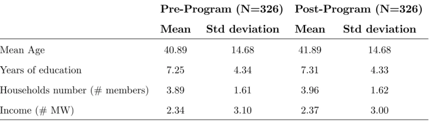
The summary of basic statisticals results is presented below. Consistent with the study’s basic …ndings, one main aspect demands special attention. The average weekly hours has increased in the program households and remained the same in the non-program households. Additionally, for land title owners, income level is higher (see Table 2).
Pre-Program (N=326) Post-Program (N=326)
Mean Std deviation Mean Std deviation
Mean Age 40.89 14.68 41.89 14.68 Years of education 7.25 4.34 7.31 4.33 Households number (# members) 3.89 1.61 3.96 1.62 Income (# MW) 2.34 3.10 2.37 3.00
Table 2: Basic statistics for 2007 and 2008
Pre-Program (N=165) Post-Program (N=165)
Ia Ib Ic IIa IIb IIc
(program) (non-prog) jt j (program) (non-prog) jt j
(N=93) (N=72) (N=93) (N=72)
Mean age 39.0 41.0 -2.0 39.9 41.9 -2.0 Time in residency
(# months) 145.3 159.5 -14.2 157.3 172.2 -14.9
Households number
(# members) 3.2 3.6 -0.4 3.2 3.6 -0.4
Income
(# MW) 1.8 2.9 -1.1 2.3 2.9 -0.6
Years of education 8.0 6.0 2.0 8.0 6.1 1.9 Hours Worked Weekly 16.0 20.2 -4.2 25.0 26.6 -1.6
Table 3: Intensive Labor Force: Working 2007 2008
Source: Author’s Estimates
First of all, as Imbens & Wooldridge (2008) pointed the DD calculates the di¤er-ence between "after" and "before" values of the mean outcomes for each treatment and control group. The di¤erence between two mean di¤erences is the impact esti-mate. In the table above, the impact estimate is 0.5 (minimum wages).
Secondly, econometric results appear in Table 3. This study default estimates include the entire set of regressors consistent with the current theory regarding level of income and land titles and the data collected during the survey. In such speci…cation, the estimate of the land title coe¢cient is 1.21, with a standard error of 0.11.
Independent variables Dependent variable
Income
Robustness check (without hours worked)
Constant 0:04
(0:23) (0:23)0:04
Sex 0:03
(0:10) (0:10)0:02
Single 0:13
(0:11) (0:11)0:14
African Brazilian 0:03
(0:10) (0:10)0:04
Years of education 0:006
(0:012) 0(0:01):007
Households number
(# members) (0:03)0:03 (0:03)0:03
Hours worked weekly 0:005
(0:084)
Moved from Canaã 0:12
(0:20) (0:20)0:13
Land title 1:21
(0:11)* 1(0:10):25*
R2=P seudo R2 0:11 0:10
N 165 165
Table 4: Income Regression
(*) Standard Error - signi…cant at 5%
The robustness part of the table provides our robustness check, excluding (as mentioned previously) to the regression analysis, the variable hours worked. The robustness outcome remains signi…cant (1.25). This result should help to reinforce the conclusion that land titling has a positive e¤ect on individuals.
clearly positive, and helps to increase the level of income.
4.4
Labor Supply of Low Income Households
Furthermore, this thesis focused on estimates of impacts of property rights on labor supply of low income households. In fact, it has not been used a poverty measure for separating households according to their standard of living. Based on the sample, the assumption that there are a some of reasons to classify all households as low income1. The table below presents a rough picture of standard of living of
households by comparing the quantiles of income distribution in 2007.
Q10 Q50 Q80 Q90 Q95
2007 0 2 MW 3 MW 4 MW 7 MW
Table 5: Quantiles of income (Minimum Wages) in 2007 for complete sample
Source: Research from the Osasco Land Title Survey
Only 5.0% from the head of households earned more than 7 minimum wages monthly. About 50.0% of household units earned no greater than 2 minimum wages monthly at that time. Furthermore, dividing this amount by family members, house-holds per capita income becomes even lower. Therefore, it has been considered all families as low income.
As mentioned before, in average, the “hours worked weekly” (by adult) increased sharply between the two phases of the …eld research. However, in average, the two scenarios have similar trends.
Again, by the designing of the experiment, it is assumed at this thesis that the program (provision of land title) was randomized at some extend. Such assumption
of means for covariates before the implementing of policy gives some support, as long as, in average, the treatment and control groups are similar to each other.
4.5
Quantile Regression Methodology
This subsection describes brie‡y the methodology of quantile regression (QR) which will be used to estimates the parameters of interest. There are two arguments which support the adoption of QR. The …rst one is when there are doubts on the homocedasticity assumption. The presence of heterocedasticity on the distribution of errors becomes the OLS estimator less e¢cient than the median estimator, for example (DEATON, 1997).
The second argument is applied even when there is no direct concerned about the e¢ciency of estimates. The QR can be used in order to stress the impact of a policy or variable on the outcome of interest. It is used to being done every time there is some suspect of impact is diverse through the distribution of interest (KOENKER & HALLOCK, 2001; ANGRIST & PISCHKE, 2009).
However, before to delve into the QR methodology, it is worth to describe the problem which has to been solved.
Under randomization, the average treatment e¤ect (ATE) of a treatment is ob-tained by the simple di¤erence of means of “hours worked weekly” on the treatment and control groups t= 1 (time/period, t = 0;1); i. e, forY(1),Y(0) ? Land.
AT Eb =E[Yb(1) Yb(0)jLand title] =E[Yb(1) Yb(0)] =E[Yb(1)] E[Yb(0)]
whereYb(1) and Yb(0) are the average of “hours worked weekly” of families which received and did not receive the treatment, respectively.
– and ATT (the average treatment e¤ect on the treated) – controlling for covariates since it can improve the e¢ciency of estimates and mitigate some noisy on the sample when randomization is not perfect. In other words, if there is some hesitation by assuming the independence between the intervention and potential results, it can be control for covariates so as to reducing the correlation between the treatment and the potential results. It is the same of assuming selection on observables2 , i.e:
Y(1); Y(0)?Land titlejX
AT E =E[Y(1) Y(0)jLand title; X] =E[Y(1) Y(0)jX]
where X represents the vector of covariates3.
This part purposes to estimate the quantile treatment e¤ect (QTE) of land title on the labor supply of adults. The strategy of estimation depends crucially on the assumption that experiment was successfully randomized. This implies that self-selection on the sample (self-selection on unobservables) it is not an issue to be concerned with.
In that way, the QTE can be obtained following the same steps described above. It could be estimated just by comparing quantiles of “hours worked weekly” distribution for the treated and non-treated or run a quantile regression controlling for covariates. It has opted for the second strategy and the quantile regression was run to get estimates for quartiles of “hours worked weekly” distribution.
The estimators of QR can be obtained by solving the following minimization
problem:
Q (YijXi) = arg
q(X)
minE[ (Yi q(Xi))]
where Q (YijXi) = F 1
y ( jXi),the conditional quantile function, is the
distribu-tion funcdistribu-tion forYi aty, conditional onXi; (u) = 1(ui0) juj+ 1(u 0)(1 )juj is called the "check function” (or asymmetric loss function) and it provides the QR estimator, : Given there is no assumption for the distribution of errors, the QR is
considered a semiparametric regression technique.
Considering the small sample size, the impact of policy will be checked on the quartiles of “hours worked weekly” distribution. According to the hypothesis sup-ported by theoretical literature, it should be observed a positive but decreasing im-pact of property rights on the labor supply distribution of the treated4.
Before discussing the QR estimates, it is worth to explore an important "tricky
point" of QR (ANGRIST & PISCHKE, 2009). The e¤ects on distribution are not equal to e¤ects on individuals. They will be the same only if an intervention is a rank-preserving – when intervention does not alter the individuals ordering. If it is not the case, it can just be said that the treated adults of a speci…c quantile are better (or worse) o¤ than control adults of the same quantile. In fact, it is a comparison between quantile of di¤erent distributions – for the treated and control groups. It is the so called QTE.
In that follow, both the OLS and QR estimates are available. As can be seen, the points estimated are di¤erent across the “hours worked weekly” distribution. The …rst two column show that OLS with and without controls are quite similar. This gives support to assumption of natural experiment.
The models have been speci…ed as follow:
Hours worked weeklyi = + l1Land title+Xi0 +"i;
Hours worked weekly = + 1 Land title+Xi0 +"i
where Xi is a vector which includes all variables, a dummy whether the family has
4.6
Results
OLS
(1) OLS(2) Q(3)25 Q(4)50 Q(5)75
Constant 10.89*** 10.39 -7.68 9.14 20.32* Mean age 0.32 -0.03 -0.89 0.02
Sex -0.21 4.05 7.84 -7.22
Marital Status -6.24** -1.52 -5.87* -9.25** Ethnicity -2.87* -1.31 -4.28 -3.20 Sex*Ethnicity 0.56 2.16 1.78 0.76 Sex*Marital status 1.08 -2.81 -3.89 3.08 Ethincity*Marital status 1.67** 0.66 2.20* 1.99* Years of education 0.32 -0.03 0.67*** 0.48 Household number (# members) 0.19 -0.06 -0.24 0.46 Income (# MW) 1.52 1.66 1.08 1.38 Land title 9.52*** 7.28*** 12.49** 10.76*** 7.47**
Child -0.52 1.28 3.02 -1.79
Child labor hours weekly -0.04 0.01 -0.23 0.45
R2 / PseudoR2 0.11 0.20 0.05 0.21 0.12
Table 6: Estimates of impact of property rights on labor supply
Note: N = 326. // The OLS standard errors are robust to heterocedasticity. The QR standard errors were obtained by bootstrap with 100 repositions. (*), (**), (***) denotes statistical
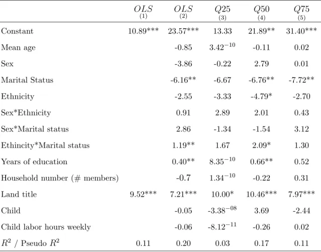
OLS
(1) OLS(2) Q(3)25 Q(4)50 Q(5)75
Constant 10.89*** 23.57*** 13.33 21.89** 31.40*** Mean age -0.85 3.42 10 -0.11 0.02
Sex -3.86 -0.22 2.79 0.01
Marital Status -6.16** -6.67 -6.76** -7.72** Ethnicity -2.55 -3.33 -4.79* -2.70 Sex*Ethnicity 0.91 2.89 2.01 0.43 Sex*Marital status 2.86 -1.34 -1.54 3.12 Ethincity*Marital status 1.19** 1.67 2.09* 1.30 Years of education 0.40** 8.35 10 0.66** 0.52
Household number (# members) -0.7 1.34 10 -0.22 0.31
Land title 9.52*** 7.21*** 10.00* 10.46*** 7.97*** Child -0.05 -3.38 08 3.69 -2.44
Child labor hours weekly -0.06 -8.12 11 -0.26 0.02 R2 / PseudoR2 0.11 0.20 0.03 0.17 0.11
Table 7: Robustness Check without Income
Note: N = 326. // The OLS standard errors are robust to heterocedasticity. The QR standard errors were obtained by bootstrap with 100 repositions. (*), (**), (***) denotes statistical
signi…cance at 10%, 5% and 1%, respectively.
Secondly, the average estimates of ATE (column 2) are similar compared to the upper quartile of the “hours worked weekly” distribution. This evidence shows that, particularly on this case, the average can underestimate the impact of policy on the result of interest. In fact, the adults who used to work less hours before receiving the treatment were those reacted who to intervention. It could be argued that low income households started work more hours after having the land title.
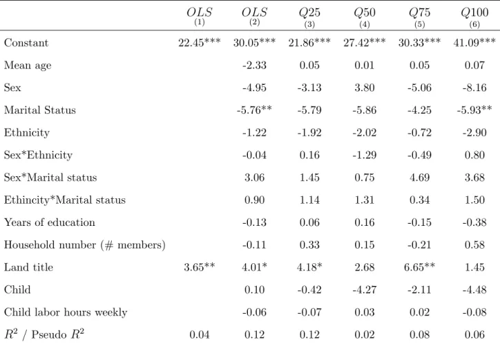
OLS
(1) OLS(2) Q(3)25 Q(4)50 Q(5)75 Q(6)100
Constant 22.45*** 30.05*** 21.86*** 27.42*** 30.33*** 41.09*** Mean age -2.33 0.05 0.01 0.05 0.07
Sex -4.95 -3.13 3.80 -5.06 -8.16
Marital Status -5.76** -5.79 -5.86 -4.25 -5.93** Ethnicity -1.22 -1.92 -2.02 -0.72 -2.90 Sex*Ethnicity -0.04 0.16 -1.29 -0.49 0.80 Sex*Marital status 3.06 1.45 0.75 4.69 3.68 Ethincity*Marital status 0.90 1.14 1.31 0.34 1.50 Years of education -0.13 0.06 0.16 -0.15 -0.38 Household number (# members) -0.11 0.33 0.15 -0.21 0.58 Land title 3.65** 4.01* 4.18* 2.68 6.65** 1.45 Child 0.10 -0.42 -4.27 -2.11 -4.48 Child labor hours weekly -0.06 -0.07 0.03 0.02 -0.08
R2 / PseudoR2 0.04 0.12 0.12 0.02 0.08 0.06
Table 8: Labor Intensive Quantile Regression (without income)
Note: N = 165. // The OLS standard errors are robust to heterocedasticity. The QR standard errors were obtained by bootstrap with 100 repositions. (*), (**), (***) denotes statistical
signi…cance at 10%, 5% and 1%, respectively.
On the top of the regressions mentioned above, we also create a speci…c regression for the labor intensive households (those working in 2007 and 2008). The results has demonstrated that the e¤ect of land title is lower compared with the one with all households. However, it is still signi…cant (specially on the 3rd quantile).
upwards, suggesting a concave shape of regression line.
5
How Does Land Title A¤ect Child Labor?
5.1
Child Labor Force Participation: The Economic Context
Investing in and focusing on human capital development is a critical factor to increase economic growth, as stated by Becker & Lewis (1973), and given such a key assumption, The United Nations Millennium Development Goals include eliminating child labor as a crucial step into a better and equal world.
According to the International Labour Organization (2002), 246 million children and teenagers between 5 and 17 years old are engaged in child labor around the world. Furthermore, 75.0% of those children work for their own family activities. Asia, Africa and Latin America are the continents with the most the child labor in the world. Asia has the highest number of children in terms of volume but Africa is the leader relative to the total size of the work force.
Figure 6: Occupation level among the 5-17 year-old population (Percentual of total 5-17 population)
Source: IBGE, PNAD 2007
children to school or to work. Rosenzweig (1981) has demonstrated that children’s time allocation depends on the production capacity of the children and their parents and the substitution degree of the work force between both.
Basu & Van (1998) have built a model using one basic assumption: luxury. They consider that poverty is the main factor that makes parents send children to work. Hence, the children’s time that is not allocated (school and leisure) to generate income is luxury, which low-income parents cannot a¤ord. Ray (2001) has created a theory for emerging economies: child labor occurs mainly because of poverty and credit market imperfections. He has shown that if poor families had access to credit, in the presence of high returns for education, they would willing to send children to school instead of work. Furthermore, the same study showed the relationship between income inequality and child labor under credit constraints. The main conclusion states that a more equal income distribution would reduce child labor.
Kassouf (2002) demonstrates that an increase in the household’s income reduces the probability of child labor and increases school attendance. Another element that a¤ects the probability of child labor is the parent’s education degree. Bhalotra & Heady (2003) …nd a negative e¤ect given the mother’s level of education and the child’s labor participation in Ghana. The e¤ect of the mother’s education pro…le is higher compared with the father’s. Kassouf (2002), in Brazil, obtains the same negative e¤ect. Family composition is another relevant factor. Patrinos & Psachara-poulos (1994) for Paraguay and Bhalotra & Heady (2003) for Pakistan, concluded that the more people there are in the family, the greater chances of having child labor.
reached the same conclusion and explain such event as "social norms", parents that worked during its childhood years face child labor more naturally. As mentioned earlier, this paper aims to provide an additional element for that discussion and test the relation between land titling and child labor force participation using the case of the City of Osasco.
5.2
Basic Findings – Child Labor Force
This section has used basically four questions to address the issue of child labor using the survey. The …rst question was: “Do you have any children?” (Please refer to Appendix A for the complete stage I and stage II questionnaires). Of the combined sample and control group, about 75.0% of the households said they have children (about 73.0% of the sample and 76.0% of the control group).
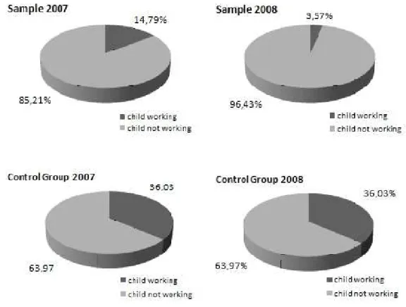
Figure 7: Are there any child/teenager helping in family income? How many?
Source: Research from the Osasco Land Title survey - 2008
Figure 8: Child Labor Force Hours Worked Weekly x Number of Households (Sample)
Figure 9: Child Labor Force Hours Worked Weekly x Number of Households (Control Group)
Source: Research from the Osasco Land Title survey - 2008
5.3
Di¤erence-in-Di¤erence Estimates: Land Title
Speci…-caton
In this paper, formally, the dependent variable is hours weekly hours of work of child labor force Y ist (the outcome of interest for household i in group s by time
t). The dependent variable would be posted as the di¤erence among weekly hours of
child labor in 2008 and 2007.
Hence, the coe¢cient is the estimated program e¤ect, which provides a measure of conditional average di¤erence in time worked by children in households in the program area versus the non-program area.
In addition, Xi includes the following controls: sex (dummy), marital status
(dummy, example: single) and ethnicity (dummy, example: African Brazilian). Another set of variables included, weekly hours of adult work is an essential variable to understand child labor according to Rosenzweig (1981) and Becker & Lewis (1973).
Patrinos & Psacharapoulos (1994) for Paraguay, Grootaert (1998) for Ghana, and Heady (2003) for Pakistan, conclude that the more people there are in the family, the higher are the chances of having child labor. Given such a framework, the number of household members is also included. The same applies for the years of education of the family head. For income, weekly hours, number of household members and years of education, also the di¤erence between the survey collection results in 2008 and 2007 is applied (example: the independent variable of hours worked is = Hours Worked 2008 – Hours Worked 2007 and so on with the other variables mentioned).
This study also estimates a regression including the households that moved from
Canaã (households that got the title, sold the property and moved right away). The goal is to check if the land title still has a positive e¤ect even considering those that are not living in the original community. Moving out fromCanaã could potentially be an e¤ect of treatment. Hence, a variable denominated "moved" will be applied as a dummy.
The Robustness check will exclude this "moved" variable.
Y i = + (Land title) + (Hours worked weekly adult) + (Households number) + (Y ears of education) + (moved) + 0Xi+ei
Furthermore, the main hypothesis to be tested is the following:
H0 : <0
H1 : 0
( -Robustness check).
5.4
Results
Pre-Program (N=251) Post-Program
Ia Ib Ic IIa IIb IIc
(program) (non-prog) jt j (program) (non-prog) jt j
Mean age 42.0 45.0 -3.0 42.8 45.9 -3.1 Time in residency
(# months) 146.2 158.4 -12.1 157.8 175.0 -17.1
Households number
(# members) 3.8 4.0 -0.2 3.9 4.1 -0.2
Number of rooms 3.3 3.7 -0.4 3.3 3.7 -0.3 Income
(# MW) 2.0 3.0 -1.0 2.0 3.0 -1.0
Years of Education 9.0 5.0 4.0 9.0 5.0 4.0 Hours Worked Weekly 9.8 9.2 0.5 19.5 10.0 9.5 Child Labor Hours Weekly 3.5 9.1 -5.6 0.5 11.9 -11.4
Table 9: Sample means - with all households that have children
Source: Author’s Estimates
First of all, the DD calculates the di¤erence between "after" and "before" values of the mean outcomes for each treatment and control group. The di¤erence between mean di¤erences is the impact estimate. In the table above, the impact estimate for children labor hours weekly is -5.8 hours.
Dependent variables
Independent variables Child Labor
(hours worked weekly) (with households that moved variable)Child Labor
Robustness check
Constant 4:68
(1:88) (1:33)4:28
Sex 0:21
(0:87) (0:87)0:20
Single 1:67
(0:96) * (0:96)1:68*
African Brazilian 0:90
(0:84) * (0:84)0:91*
Years of Education 0:17
(0:10) (0:10)0:16
Households number
(# members) -0(0:25):45 (0:25)0:45
Hours worked weekly 0:01
(0:03) (0:03)0:01
Moved from Canaã 0:48
(1:63) ( )
Land title 6:08
(0:93) * (1:22)6:04*
R2=P seudo R2 0:13 0:13
N 251 251
Table 10: Child Labor and Land Title
(*) Standard Error - signi…cant at 5%
help to reinforce the conclusion that land titling has a positive e¤ect on individuals, and not only on property.
Hence, the e¤ect of land titling, given the conditions and variables applied, is clearly positive, and helps to minimize the number of weekly hours worked by children in the case of Osasco.
6
How Does Land Title Improve Happiness?
6.1
Happiness in Economics: Theory and Data
Aristotle to Bentham, Mill, and Smith, incorporated the pursuit of happiness in their work. Even within a more orthodox approach framework, focusing purely on income can miss key elements of welfare. People have di¤erent preferences for mate-rial and non-matemate-rial goods. They may choose a lower-paying but more personally rewarding job, for example. They are nonetheless acting to maximize utility in a classically Walrasian sense.
The study of happiness or subjective well-being is part of a more general move in economics that challenges these narrow assumptions. The introduction of bounded rationality and the establishment of behavioral economics, for example, have opened new lines of research. Happiness economics which represents one new direction -relies on more expansive notions of utility, and the interaction between rational and non-rational in‡uences in determining economic behavior.
that, even if agreement exists on how a policy a¤ects behavior, there is often a lack of consensus on the consequences of the policy will a¤ect welfare.
The literature of well-being economics is currently growing at a remarkable rate. If one takes the view that human happiness is ultimately the most important topic in social science.
Richard Easterlin was the …rst modern economist to revisit the concept of happi-ness, beginning in the early 1970s. Speci…cally Easterlin (1974) observed happiness responses are positively correlated with individual income at any point in time: the rich report greater happiness than the poor within the United States in a given year. Yet since World War II in the United States, happiness responses are ‡at in the face of considerable increases in average income. A similar pattern has been observed in a large number of countries, including France, the United Kingdom, Germany and Japan, and for di¤erent periods of time (EASTERLIN, 1995; BLANCHFLOWER & OSWALD, 2004).
The economics of happiness does not purport to replace income-based measures of welfare but instead to complement them with broader measures of well-being. These measures are based on the results of large-scale surveys, across countries and over time, of hundreds of thousands of individuals who are asked to assess their own welfare.
The happiness data typically available for the United States have only three response categories. Starting 1972, the General Social Survey carried out by the National Opinion Research Center has asked: "Taken all together, how you would
say things are these days - would you say that you are very happy, pretty happy or not too happy?" The European Eurobarometer Surveys recommends, on the top of the question mentioned above, asking also: "On the whole, are you very satis…ed,
of happiness is the degree to which an individual judges the overall quality of his or her life as favorable as pointed Veenhoven (2003).
Micro-econometric happiness equations have the standard form: W it= + xit+
"it, where W is the reported well-being of individual i at time t, andX is a vector
of known variables including socio-demographic and socioeconomic characteristics. Happiness data are being used to tackle important questions in economics. Part of this approach is quite natural, as many questions in economics are fundamentally about happiness.
Happiness data addressed some of the issues in the unemployment-in‡ation lit-erature. Wolfers (2003) presents a comprehensive set of estimates, using data on the happiness responses of more than half million people in a maximum of 16 European countries for the period 1973-1998 (for total of 274 country-years). The calculations show that in‡ation and unemployment both reduce happiness. Di Tella, MacCul-loch & Oswald (2003) estimates that an additional percentage point of unemploy-ment causes twice as much of a reduction in happiness as an additional percentage point of in‡ation in a smaller sample that includes country-speci…c time trends as controls. Furthermore, other cross-sectional and panel studies reveal that unem-ployed individuals tend to report low happiness scores (CLARK & OSWALD, 1994; WINKELMANN & WINKELMANN, 2003).
Some authors have used happiness data to study other, more permanent institu-tional features of the economy, such as the role of direct democracy. Frey & Stutzer (2000) exploit the large cross-sectional variation in the institutional rights to politi-cal participation across the 26 Swiss cantons. They …nd that average happiness and an index of direct democracy in a canton are positively correlated. Furthermore, political arrangements also matter. Much of the literature …nds that both trust and freedom have positive e¤ects on happiness (HELLIWELL, 2003; LAYARD, 2005).
In Brazil, Corbi & Menezes Filho (2005) investigates the role that economic vari-ables play in the determination of happiness, using reported happiness as a proxy to individual well-being. The authors use microdata extracted from the World Val-ues Survey for …ve countries, emphasizing the Brazilian case. Their …ndings suggest that there is a positive and signi…cant correlation between happiness and income. Unemployment is also a large source of unhappiness. In most cases, happiness ap-pears to be positively correlated to being married. Moreover, happiness is apparently U-shaped in age (minimizing at 50’s).
6.2
Basic Statistics – Happiness and Land Title
This study has used basically two questions to address the issue of happiness along the survey. The …rst question was "Taken all together, how you would say
Additionally, the diagram below summarizes the household’s answer (stage I and stage II) about level of happiness. There is clear, among the sample, an increase (from 2007 to 2008) in the number of very happy households. On the other hand, the control shows a di¤erent trend, a decrease among the very happy people.
Figure 10: Taken all together, how would you say things are these days - would you say that you are...?
Figure 11: Taken all together, how would you say things are these days - would you say that you are...?
Source: Research from the Osasco Land Title Survey - 2008
Figure 12: On the whole, about the life that you lead, are you...?
Figure 13: On the whole, about the life that you lead, are you...?
Source: Research from the Osasco Land Title survey - 2008
6.3
The Multinomial Probit Model
As Wooldridge (2005) stated that one kind of multinomial response is an ordered response. As the name suggests, ifyis an ordered response, then the values assigned to each outcome are no longer arbitrary. For example,ymight be a level of happiness
The fact that two is a higher level than one conveys useful information even though level of happiness itself only has ordinary meaning.
Lety be an ordered response taking on the values (0,1,2) for a known integer J.
The ordered probit model fory (conditional on explanatory variablesx - in the case
of happiness, those variables would be, for example, sex, age, employment, income and etc.) can be derived from a latent variable model.
Assume that a latent variable y is determined by:
y =x +ei e=X ~ N ormal (0;1) (9)
where is Kx1 and x does not contain a constant. Let 1 < 2 < ::: < j be
unknown cut points (or threshold parameters) and de…ne:
y= 0 se y 1
y= 1 se 1 < y 2
. . .
y=J se y > j
In the case of happiness, if y takes on values 0, 1 and 2, then there are two cut points, 1 and 2:
P(y = 0jx) =P(y 1jx) = P(x +e 1jx) = ( 1 x ) P(y = 1jx) =P( 1 < y < 2jx) = ( 2 x ) ( 1 x )
:
:
:
P(y = J 1jx) =P( j 1 < y jjx) = ( j x ) ( j 1 x ) P(y = Jjx) = P(y > jjx) = 1 ( j x )
where is the cumulative distribution function. The sum of the probabilities is 1.
WhenJ = 1, it is a binary probit model:
P(y= 1jx) = 1 P(y= 0jx) = 1 ( 1 x ) = (x 1) (10)
is the intercept inside . That is the main reason that x does not contain an
intercept in this formulation of the ordered probit model. As Greene (2002) points, when there are only two outcomes, zero and one, a single cut is set to zero to estimate the intercept, such approach leads to the standard probit model.
The parameters and can be estimated by maximum likelihood. For each i,
li( ; ) = 1[yi = 0] log[ ( 1 x )] +
1[yi = 1] log[ ( 2 x ) ( 1 x )] +:::+
1[Yi = N 1] log[ ( j x ) ( j 1 x )] +
1[yi = N] log[1 ( j x )]
While the direction of the e¤ect of Xk on the probabilities P(y = 0jx) and
P(y=Jjx)is determined by the sign of k, the sign of k does not always determine
the direction of the e¤ect for the intermediate outcomes 1;2:::; J 1.
For example, suppose there are three possible outcomes for level of happiness,
J = 3 (or y= 0, y= 1,y= 2) and k>0, then:
y = 0 =) @P
@Xk(Y = 0jx) = ( 1 x )<0 (11)
y = 2 =) @P
@Xk(Y = 2jx) = ( 2 x )>0 (12)
where is the density function. However, fory= 1, @P
@Xk(Y = 1jx) could be either sign. Ifj 1 x j < j 2 x j, then ( 1 x ) ( 2 x ) will be positive, and if not, negative.
6.3.1 Predicted Probabilities
average individuals". This method consists on calculating the probability of each household following on each group.
As an example, consider 3 categories, once estimated the vector and the cut points, the probability for householdi of following within each one of them is:
P(yit = 1jxit) =P(yit 1jxit) = ( 1 xit )
P(yit = 2jxit) = ( 2 xit ) ( 1 xit )
P(yit = 3jxit) = ( 3 xit ) ( 2 xit )
Hence, "optimal" group predicted for householdiis the outcome with the highest
probability.
6.3.2 Partial E¤ects of Continuous Covariates
The parameters of vector estimated at ordered probit are not equal to the marginal e¤ects of the regressors. The main input is given by the marginal e¤ect of each covariate in response probabilitiesP(yit =Jjxit).
@P(yit = 1jxit)
@xk = k ( 1 xit )
@P(yit = 2jxit) = k[ ( 1 xit ) ( 2 xit )]
@P(yit = 3jxit) = k[ ( 2 xit ) ( 3 xit )]
The marginal e¤ect of xk have the opposite sign of the estimated k for the …rst
group and same sign for the last. Intermediate e¤ects will rely on the probability densities.
6.3.3 Partial E¤ects of Discrete Covariates
In order to calculate partial e¤ects of discrete variables, the approach is to com-pare the probabilities calculated along with dummy variables (values 0 and 1, for example). The partial e¤ect of the dummy variable xk for the case of 3 groups, for
instance, is given by
P E i,1(xi; k) = P(yi = 1jxi;k = 1) P(yi = 1jxi;k = 0)
P E i,2(xi; k) = P(yi = 2jxi;k = 1) P(yi = 2jxi;k = 0)
P E i,3(xi; k) = P(yi = 3jxi;k = 1) P(yi = 3jxi;k = 0)
It is assumed by such approach that the di¤erence in probabilities is all due to the e¤ect of the dummy variable, therefore that is the partial e¤ect.
6.4
Multinomial Probit Model: Land Title Speci…cation for
Happiness
The dependent variable is level of happiness change from 2007 to 2008 surveys round. As mentioned earlier, two questions were applied regarding happiness dur-ing both periods (“would you say that you are very happy, pretty happy or not too happy?” – please refer to question number P.18 at Appendix A for details).
level of happiness was lower compared to 2007 (example: if, in 2007, the answer was “pretty happy” and 2008 is “not too happy”). Second, if the answer has remained exactly the same and third if a greater level occurred (example: “not too happy” in 2007 and “pretty happy” in 2008).
For each possibility mentioned above a numerical outcome was assigned: 0,1 and 2. Additionally, an ordered probit was applied to estimate e¤ects of various factors on the probability of each outcome.
Also, indicates whether the household lives in a neighborhood that has been reached by the program – being the dummy for whether the land title has a¤ected the each group.
Hence, the coe¢cient , in this case of happiness, is the estimated of program e¤ect, which provides the e¤ect of land title on the probability of each happiness level change.
In addition, other social and economic factors were applied such as sex (dummy), marital status (dummy: single), ethnicity (dummy, example: African Brazilian), years of education (of the family head) and number of household members.
Another variable included, and covergent with Corbi & Menezes Filho (2005) …ndings, is the income level (please refer to question number P.38 at Appendix A for details). Furthermore, Wolfers (2003) and Tella, MacCulloch & Oswald (2003) conclude that employment has positive impact on happiness. Hence, if the household is formally employed will also be applied.
6.5
Results
The Table 11 presents the results from the estimation of the ordered probit de-scribed above. Basically, the outcome provides the predicted coe¢cients of key in-dependent variables given a 5.0% level of signi…cance. Furthermore, the number of categories (three) implies two cut points for the probit model.
Econometric results appear in the Table 11. Such outcome has demonstrated that the estimate of land title coe¢cient is -1.04, with a standard error of 0.17. That, in the case of ordered probit, implies that land title signi…cantly impacts the level of happiness.
The robustness part of the table provides the robustness check, adding the “sat-isfaction” level. The robustness outcome also address the signi…cant impact of the variable land title related to “satisfaction”. The estimate coe¢cient for land title is -0.62 with a standard error of 0.15.
Dependent variables
Independent variables Happiness Satisfaction Robustness check
Sex 0:13
(0:17) (0:15)0:17
Single 0:01
(0:18) (0:18)0:17
African Brazilian 0:25
(0:22) 0(0:21):26
Years of Education 0:01
(0:02) (0:02)0:01
Households number
(# members) (0:04)0:03 (0:04)0:04
Income
(number of Minimum Wage) (0:00004)0:00005 0(0:0004):00005
Hours worked weekly 0:20
(0:15) 0(0:15):04
Land title 1:04
(0:17) * (0:15)0:62
LR chi2 51:43 25:40
Prob > chi2 0:00 0:00
Log likelihood 227:80 243:25
Cut 1 2:51
(0:45) (0:43)2:18
Cut 2 0:72
(0:43) 0(0:41):07
R2=P seudo R2 0:10 0:09
N 326 326
Table 11: Happiness and Land Title
(*) Standard Error - signi…cant at 5%
of happiness. However, it does not fully address the probability of a household becomes part of “higher (or lower) happiness level group” given its participation on the program.
6.5.1 Predicted Probabilities – The Partial E¤ects of Land Title
The Table 12 below shows the predicted probabilities, i.e, the probability for an average household being in each of the ranges described above (higher level of happiness comparing 2008 and 2007 surveys, same level and lower level).
An average household re‡ects an individual that carries the average levels of income, years of education, number of family members, age, marital status, race and sex from the complete sample (N=326).
Given the average household pro…le, this particular research tests two scenarios: a) average individual in the program (with land title); b) average individual without the program (no land title).