A SYSTEMATIC COMPONENT OF THE JUMP-RISK
PREMIUM IN AN AJD MODEL
Livio Cuzzi Maya
Dissertação submetida como requisito parcial para
conclusão do Mestrado em Economia
Ficha catalográfica elaborada pela Biblioteca Mario Henrique Simonsen/FGV
Maya, Livio Cuzzi
A systematic component of the jump-risk premium in an AJD model / Livio Cuzzi Maya. – 2015.
25 f.
Dissertação (mestrado) - Fundação Getulio Vargas, Escola de Pós-Graduação em Economia.
Orientador: Caio Ibsen. Inclui bibliografia.
1. Risco (Economia). 2. Processo estocástico. 3. Mercado de opções. 4. Derivativos (Finanças) – Preços. 5. Modelos econométricos. I. Almeida, Caio Ibsen Rodrigues de. II. Fundação Getulio Vargas. Escola de Pós-Graduação em Economia. III.Título.
A systematic component of the jump-risk premium in an AJD
model
∗Livio Cuzzi Maya
Abstract
We develop an affine jump diffusion (AJD) model with the jump-risk pre-mium being determined by both idiosyncratic and systematic sources of risk. While we maintain the classical affine setting of the model, we add a finite set of new state variables that affect the paths of the primitive, under both the actual and the risk-neutral measure, by being related to the primitive’s jump process. Those new variables are assumed to be commom to all the primitives. We present simulations to ensure that the model generates the volatility smile and compute the “discounted conditional characteristic func-tion” transform that permits the pricing of a wide range of derivatives.
Key words: Jump - Systematic Risk - Affine model - Macroeconomic Risk - Derivative pricing
∗I deeply thank the Carlos Chagas Filho Foundation for the Support of Research in Rio de Janeiro State (FAPERJ) for
Contents
1 Introduction 3
1.1 Systematic state variables . . . 4
1.2 Literature Review . . . 5
2 The general model 6
2.1 Stock return dynamics: data-generating process . . . 8
2.2 The risk-neutral dynamics . . . 10
3 A two stage orthogonalization procedure 11 3.1 Extracting the volatility path. . . 12
3.2 Systematic variable projection . . . 12
4 An application to macroeconomic processes 14 4.1 Taylor rule application . . . 16
5 Simulations 17
6 Calculating the discounted characteristic function 19
1
Introduction
The development of financial economics and asset pricing theory in recent decades has led re-searchers to accept the idea that asset prices dynamics contain important information regarding agents preferences and beliefs. The “weight” that agents put in different states of nature when evaluating assets reflect not only the effect of different endowments or technologies on their util-ity in equilibrium, but also their perception of the likelihood of different scenarios. Literature in empirical finance has been interested in developing techniques to assess such perception through the observation of asset prices, both derivatives and its primitives. In the case of using derivatives, studies (to be named in the next pages) indicate that if we assume those primitives to be driven by continuous processes, we fail to explain the prices (or implied volatility) pattern observed in real world data. Adding a jump component to the primitive’s process helps to reconciliate the the-oretical prices and the real-world prices, as its distribution changes (especially in what concerns its volatility).
Adding the jump component parcially solves a question, but it also gives rise to another one: what drives the premium investors demand for facing the possibility of jumps? As we said, prices dynamics contain information of agents perception of different scenarios. In the moment we add a jump component in the conditional distribution of a primitive, we instantly add many potential different scenarios in the future and so we have to evaluate how agents “weight” those new scenar-ios. Looking at the risk neutral probability measure generated by agents preferences and beliefs is a traditional way literature has developed to quantify those “weights”. In fact, a more technical way to pose the same question would be: under the risk neutral probability measure, what determines the joint distribution of jumps and the other sources of uncertainty? The aim of this work is to marginally contribute in the answer of this question by presenting an affine jump-diffusion (AJD) model that highlights the influence of systematic state variables on the jump-risk premium.
In subsection1.1we will define and explain what we are now calling a systematic state variable. The basics of the model (the AJD setting) were chosen for its popularity and easiness of implemen-tation. Although we acknowledge the fact that literature has advanced with respect to the affine structure, we believe that its high influence and relevance justify the adaptation of the classical model to incorporate the role of systematic state variables, at least as a small contribution in the attemp to answer the question posed. Besides, the setting of an AJD model is relatively simple to be read. Hence, we will be able to clearly highlight the role played be the variables we introduce, which we believe to be a gain.
We present an affine jump-diffusion (AJD) model that falls into the class studied in the influen-tial work ofDuffie, Pan & Singleton(2000). Our idea is to link the systematic state variable process to the primitive jumps’ distribution and to explore a possible relationship between the nominal interest rate and the systematic variable1 to identify the role that such systematic variable plays
1The relation between the nominal interest rate and the systematic variable might be very useful if we model a
in the price of a derivative. In order to accomplish such a goal, we have to face the heavy ana-lytics involved in solving the differential equations that characterize the derivative’s prices in AJD models. In turn, however, having such prices allows us to identify the premia related to shocks on those systematic variables, which would be our final goal. Of course, systematic risks are sys-tematic. Therefore, the parameters that define its process should be the same for every primitive process (although the way it affects the primitive’s conditional distribution should be allowed to differ) and so panels of primitives should prove themselves useful to estimate such parameters. The estimation, however, will not be a part of this preliminary work.
This paper is organized as follows. The remainder of section1discusses the definition and role of systematic state variables (subsection 1.1) and gives a brief literature review on related asset pricing theory and empirics (subsection 1.2). To express our results, we first develop a general model in section 2 that is able to incorporate systematic variables. In section 3, we propose a method to account for the issue of processes driven by correlated shocks. In section4, we give an application of the model to incorporate macroeconomic variables (or variables that we assume to have linear relation with the interest rate process). In section5, we present results from simulations that show that the model is able to reproduce the volatility smile. In section 6 we compute the transform that can be used to price different kinds of derivatives. Section7concludes.
1.1 Systematic state variables
The presence of jumps was originally introduced in stochasic volatility (SV) models in Bates
(1996). In the original setting, the jump process (its intensity and size) was considered indepen-dent of the Brownian shocks and its distribution stationary. The work ofPan(2002) maintains the general setting ofBatesmodel, but the jump’s intensity is allowed to be dependent on the current stock’s volatility, on both the data-generating conditional distribution (or “real world”) and the risk-neutral conditional distribution. Consequently, the work captures the premium investors demand for being exposed to the jumps in periods with different levels of market volatility.
While many other variables could be assumed to impact the jump-risk premium, we focus on a narrower class of varibles. We define systematic state variables as variables characterized, as the name suggests, by the fact that its path is the same for every stock or asset considered and its distribution is not independent from the prices processes. Unlike volatility, whose component on the jump-risk premium can be considered idiosyncratic (each stock has its own underlying volatility process), a systematic variable component is not stock specific. Shocks on these variables happen in the say way for every primitive we consider in the cross section. What can vary, nevertheless, is the premium related to this risk in each stock2.
A systematic state variable can have several interpretations. For instance, consider a manufac-turing sector that relies heavily on the supply of a commodity in order to produce. Shocks in the price of this commodity will be equal for every company in the sector. If we believe the commod-ity’s price can affect the tail risk of the stocks in this sector, we can assume it to be a systematic
state variable in a model that contemplates the dynamics of the sector’s stocks. When investors buy stocks from one company of such sector, they get exposed to the risk that the stock price will jump. Such a risk can be assessed by investors very differently depending on the prices of the commodity. If a shock causes the commodity’s price to soar, investors might demand a greater premium for the possibility of jumps.
Another possible interpretation for the state variables is a macroeconomic process such as in-flation or public debt. A macroeconomic variable shock will tipically be the same for every asset, which guarantees the definition of a systematic variable is satisfied. Applying our setting for the use of a macroeconomic variable can be very useful. While recent literature has been focused on identifying the influence of macroeconomic variables through a narrow class of assets3, it would allow us to diverge from such trend by introducing a model that relates macroeconomic variables to usually studied derivatives, without focusing on any particular one. The introduction of one or more macroeconomic varibles would allow us to test the perception of agents regarding the paths of such variable. In this work, we present an application of the model to capture the features of Taylor-type interest rate rules.
As the use of classical arbitrage-free models such as the Black & Scholes (1973) and Heston
(1993) suggests, it is indeed possible to use derivatives prices to assess the market’s perception of risk related to their primitives. Our model fits the gap of an arbitrage-free model that presents a primitive’s distribution directly influenced by systematic factors instead of only idiosyncratic risks, such as stochastic volatility or stock jumps. Pricing the derivatives from the assumed distribution of the primitives allows for the extraction of the risk premia related to the systematic variable through the same techniques widely used in empirical finance to estimate classical models. Therefore, al-though we do not touch data, our calculations result into a transform, the discounted conditional characteristic function, that might be used to elaborate inference on the derivative’s prices and, thus, extract the premia related to the systematic risk.
1.2 Literature Review
This theoretical work is focused on a model that can be applied to a general class of assets. We’ll be very in touch with literature of arbitrage-free asset pricing, given that the variety of models gives us the tools to develop a model as broad as possible.
Literature in asset pricing theory and empirical finance has been especially interested in finding hypothesis on asset returns distributions that are consistent with observed prices movements. Clas-sical models have been tested not only through time series analysis of stock panels but also from derivatives cross-sections and panels. In fact, recent literature reveals that derivatives data may provide crucial information on the risks related to their primitives. For instance,Broadie, Chernov
3Here are some examples of articles that use asset prices to identify agents perception of macroeconomic variables.
& Johannes(2007) andBollerslev & Todorov(2011) use respectively parametric and nonparamet-ric models to study the impact of jumps on the risk premium of equity. Their work is important to us for two reasons. First, because it corroborates the importance of analysing derivatives to extract information of the risk premia. Second, because our work rely on the assumption that jumps are influenced by systematic factors. If jumps were found not to be important to explain real world data, our use of jumps in the model wouldn’t be well motivated.
It is already well accepted by researchers the idea that most stock returns distributions can be modelled through both stochastic volatility and jump events on their generating process. The exis-tence of those risks, especially of sudden shifts of the stocks prices, and their complex relationship has strengthened the hypothesis that markets are incomplete, as opposed to the assumption from classical Mehra & Prescott (1985) equity premium puzzle. In this context, several asset pricing models based on no-arbitrage arguments to relate the derivative to its underlying asset have been developed. Many of these models, especially the classic ones, fall in the category of affine models studied byDuffie, Pan & Singleton(2000). That’s also going to be the case for our model. Perhaps the most simple of such models, Black & Scholes(1973) assume stock’s volatility to be constant and that there is a single risk factor to be taken into account when pricing options.Heston(1993) assumes a stochastic volatility model and thus present two risk factors: the stock’s diffusion shocks and the volatility’s diffusion shocks. Bates (2000) model incorporates a jump process (and thus a jump premium) as a third factor into its previous counterpart. Finally, Duffie, Pan & Singleton
(2000) derive a double jump model, with jumps on both the stock and the volatility’s diffusions. For that last model, one can also look at Eraker, Johannes & Polson (2003) for a more general case. As it has already been highlighted, recent literature covers for example the case of jumping volatility, which we ignore in our model.
This work is located in the gap between Bates(2000) andDuffie et al.(2000) models. We as-sume the presence of stochastic volatility and jumps in the stock generating process.Pan (2002) adapts Bates model by making the jump-risk premium to be linearly dependent on the market volatility. We adapt this model by incorporating a finite number of processes in the jump-risk pre-mium. By this modification we perform a generalization of the conditional distribution of the jumps occurrences, still leaving it as a “state-dependent” process. It is important to underline, however, that the model treated in this work is far from being the most general possible.
The idea of capturing the effect of systematic risks isn’t new also. For more recent work on systematic state variables, one can look atBollerslev, Todorov & Li(2013) andBarigozzi, Brownlees, Gallo & Veredas(2014).
2
The general model
the data. Thus, it is important to be clear about how we model the stock return process.
As already mentioned, our model belongs to the class of AJD models. We incorporate stochastic volatility, jumps, non-constant interest rate and dividend processes. The model presented in Pan
(2002) would be a great starting point to understand the stock return dynamics presented in this work. The difference of our work, however, is that we assume the existence of one or more sys-tematic state variables. It is straightforward to realize that there are tons of ways to model the impact such variable in asset pricing, even if we restrict ourselves to the class of AJD models. For this reason, we shall discuss briefly the assumption on the systematic variable before introducing the environment setting with the data-generating processes and risk-neutral processes.
As we want to identify the market’s perception of the likelihood of different scenarios of the systematic variable, it is crucial to incorporate its influence in the state price density. By that, we are implicitly assuming that the way individuals price the asset’s payoff will depend on how they evaluate the systematic variables possible paths. In comparison with the data-generating process of the systematic variable, its risk-neutral process can also present a “premium” component that impacts the pricing of derivatives.
The other fundamental hypothesis is that the systematic variable is linked to the stock’s jump process, in both the data-generating and the risk-neutral distribution. Afterall, our main motivation is to answer the question of what determines the jump-risk premium. By linking the systematic variable to the jump’s intensity we gain two features: first, we explicitly identify the risk premia for future econometric work; second, it allows our model to be used in the study of what processes influence a stock’s tail risks, which is a still open question in empirical finance. In fact, including the systematic variable as a determinant of the jump’s intensity constitute a nice robustness test to the hypothesis that the intensity is time invariant or to the hypothesis that it depends on other time variant processes, such as the volatility4.
Given the discussion above, it is important to highlight the set of properties we will require the systematic variable to possess when entering the primitive’s conditional distribution in our model. There will be two basic properties:
1. Pricing kernel property. We want the systematic variable to affect the risk-neutral condi-tional distribution of the stock process, or its kernel price5. If that isn’t true, then agents do not price its risk. In that case, even if we assume that the “data-generating” process is af-fected by the macro variable, derivative’s price won’t be, and computing its price will be a meaningless exercise.
2. Jumps property. As our main goal is to study the jump-risk premium and the impact it receives from systematic variables, it is clear that the systematic variable must be related to the distribution of the jump process. We will satisfy this property by assuming that the systematic variable impacts the intensity of the jump process.
4SeePan(2002) for the case of a linear relationship andSanta-Clara & Yan(2010) for the nonlinear case.
Properties1and2will be standing in the setting we present in next subsection.
Another property that we are going to use, although not one worthwhile to appear in the list above is that the variable at hand moves in cycles. Although this property is not fundamental, we believe that such setting would be able to capture the dynamics of many autonomous variables.
2.1 Stock return dynamics: data-generating process
In this subsection we mathematically characterize the assumptions on the stock return dynam-ics. We start by fixing a probability space (Ω,F,P) and a filtration Ft. Probability measure P is
considered the “actual” probability measure. We will discuss the conditional distribution of the stock return under a risk neutral mesureePin subsection2.2.
Let Stbe the ex-dividends stock price,Vt its instantaneous volatility,qtthe rate at which
divi-dends are paid for this stock,rtthe interest rate process andmit thei-th systematic variable, all of
them evaluated at periodt.
The dynamics of the state variables underPare given below
dlnSt= "
rt−qt+ηsVt+ (µ−µ˜) λ0+λ1Vt+ N X
i=1
γimit !
−Vt 2
#
dt+pVtdWt1 (1)
+ ln(1 +Y)dNt−µ λ0+λ1Vt+ N X
i=1
γimit !
dt
dVt=κv(¯v−Vt)dt+σvρ p
VtdWt1+σv p
1−ρ2pV
tdWt2 (2)
dqt=κq(¯q−qt)dt+σq√qtdWt3 (3)
drt=κr(¯r−rt)dt+σr√rtdWt4 (4)
dmit=κim( ¯mi−mit)dt+σim√mitdWt4+i i= 1, . . . , N (5)
whereWt= [Wt1, . . . , WtN+4]T is an adapted standard multivariate brownian motion underPand
Ntis a Poisson process with instantaneous state-dependent intensity6λt≡λ0+λ1Vt+PNi=1γimit.
We assume λ0, λ1, γi > 0 for i = 1, . . . , N. In order to keep things as simple as possible, we also
assumem¯i >0for everyiand that the initial conditions are positive for each systematic variable7.
As one can see, our model is an extended version ofBates(1996) model. It captures two major features of the stock return dynamics: stochastic volatility and price shifts. We now discuss the main differences from traditional models.
We start by analysing equation (1). It is basically the Itô’s lemma application of the log function on the original stock price process below:
dSt= [rt−qt+ηsVt+ (µ−µ˜)λt]Stdt+ p
VtStdWt1+St−Y dNt−µλtStdt
6We use the informal notationλ
t for the jump’s intensity even though it depends on the path of the state variables besides the periodt.
7Notice that the case in which the systematic variable is assumed to take only negative levels is only a particular case
Under P, the ex-dividend stock process must have the mean return of the interest rate minus
the rate on which dividends are paid plus the premia for brownian shocks and for jumps. Theµλt
term accounts for the expected change in the jump processSt−Y dNt, which we now explain. The
jumps occurrences are modelled through a Poisson processNt. Its instantaneous intensity is linearly
depend on both the volatility Vt and the systematic variablesmit, i = 1, . . . , N. The dependency
on the volatility isn’t new in literature (see Pan (2002)). We introduce the dependency on the systematic variableemitso that property2from the last subsection is satisfied.
Conditional on the occurrence of a jump, the stock price shifts fromSt− toSt−(1 +Yk), where
k=Nt(i.e.,YkSt−is the jump size of the k-th jump). The jump sizes are independent of the Poisson
process, as it is usually true in AJD models. The jump size factor1 +Y is assumed to be log-normal under the risk-neutral measure, with constant meanµj and varianceσ2j. Therefore, the jump size
random variableY has meanµ= eµj+
σ2j
2 −1. It should now be clear that theµλ
tSt compensates
for the trend the jump process imposes on the stock price path.
Under the risk-neutral measure Pe we assume to be valid in subsection 2.2, random variable
1 +Y is still assumed to be log-normal, but with different meanµ˜j and variance ˜σ2j. Parameterµ˜
accounts for the expected jump size of variableY, conditional on the occurrence of a jump, undereP
(so that we haveµ˜=eµj˜ + ˜
σ2j
2 −1). As for the intensityλ
t, we assume it to be the same under bothP
andPe, followingPan(2002). Hence, the stock risk premia associated with the jump is given by the
term(µ−µ˜)λtSt. It must be clear now that, with this setting we allow the risk premia associated
with the jump component of the stock prices to vary with more or less volatile markets as well as with the current state of the systematic variables. We are, therefore, satisfying property1.
Finally, the termηsVtrepresents the premium for the risk of brownian shocks. Overall, the state
variablelnStcaptures two premiums. The first one,ηsVt, corresponds to the risk of brownian shocks
and the second one, (µ−µ˜)λtSt, corresponds to the risk of jumps. Under the actual probability
measure P, the expected rate of growth of the stocks is given by the sum of the interest rate, the
two premia for risk minus the dividend payment rate. Following empirical findings, we always expect to find positive premia for both types of shocks. That means we expectηs>0andµ >µ˜.
We now turn our attention to the volatility processVt, the dividend rate processesqtand the
in-terest rate process, defined by equations (2), (3) and (4), respectively. All of them are autonomous mean reverting processes, as modelled inCox, Ingersoll & Ross(1985). Their long run averages are given by parametersV¯,q¯andr¯, while the mean-reversion rates areκv,κqandκr, all assumed to be
positive. Provided that their long term means and their initial conditions are all greater than zero,
Vt,qt andrt are all going to be non negative with probability one, which seems to be a desirable
property. Parametersσv,σqandσrgive the expected standard deviation of those processes. Notice,
internal consistency of the model, the interest rate process parameters should be equal for every stock in the cross-section, unlike the volatility and the dividends-rate parameters, which should vary from stock to stock. In fact, strictly speaking, the interest rate is a systematic variable if we use the definition provided in subsection1.1.
We now investigate the systematic variables mit. First thing to be noticed is that we assume
only a finite number of systematic variables to be relevant in the dynamics of the stock. Second, as already pointed out, we want to provide our systematic variables a “cycle-behavior” character, al-though other linear settings would be an easy alternative to our model. As we modelled in equation (5),mitwill be mean reverting provided thatκim>0. We can say thatmit is also an autonomous
mean reverting process. Indeed, it will be characterized by the fact that it is expected to go up whenever it is below the long run average m¯i and to go down when it is above m¯i. Its diffusion
part is not allowed to correlate with any other diffusion, although it might reasonable to think that some stock (and other primitives) prices vary along systematic shocks, which makes the correlation case an interesting one (and not analytically costly).
2.2 The risk-neutral dynamics
In addition to the actual probability measure, we assume the existence of an equivalent mar-tingale measurePe. Since the market at hand is incomplete due to the log-normal jump size, there
are infinite equivalent martingale measures, and so we can advantage of that fact to calibrate the model to fit the data.
Under the risk-neutral probability measure we choose, eP, the dynamics of the state variables
lnSt,Vtandmit, fori= 1, . . . , N are given bellow:
dlnSt=
rt−qt−
Vt 2
dt+pVtdWft1+ ln(1 +Y)dNt−µλ˜ tdt (6)
dVt= [κv(¯v−Vt) +ηvVt]dt+σvρ p
VtdfWt1+σv p
1−ρ2pV
tdWft2 (7)
dmit= [κim( ¯mi−mit) +ηimmit]dt+σim√mitdfWt4+i i= 1, . . . , N (8)
Under eP, fW1, Wf2 and Wfi, i = 1, . . . , N are all independent standard Brownian motions. Also,
W3 andW4 still are considered Brownian motions, so that the dynamics of the processes qt and
rt are still given by equations (3) and (4) respectively.Ntis still a Poisson process with intensity
λt = λ0 +λ1Vt+PNi=1γimit under Pe, which guarantees that property 1 given in the beginning
of section 2 is satisfied, for the systematic variables are a part of the pricing kernels. As argued in subsection2.1, the moments of the jump size change underPe. The expected jump size on lnS
conditional on the ocurrence of a jump is given byµ˜j and the variance is σ˜j2. Correspondingly, the
mean ofY, conditional on the jump occurrence, isµ˜.
Under the risk-neutral measure, the ex-dividend stock price is expected to grow at ratert−qt, as
it should be by the definition of a risk-neutral probability measure. The term−µλ˜ tdtcompensates
the overall process, only volatility.
The volatility process underePis represented by equation (7). Once more, we model it as a
mean-reverting process, but now we add a premiumηvVtthat compensates for the stochastic component
of the volatility. Since volatility per se cannot be traded as a primitive asset, the premium for the fact that the stock’s volatility is volatile appears only in the dynamics of option prices. In other words, while stock prices won’t reflect the term ηvVt, derivatives’ prices will. Previous literature
has already acknowledged the existence of this premium (one can see evidence of this term in
Lamoreux & Lastrapes(1993)). Once again, the volatility diffusion is allowed to be correlated with the stock diffusion. We assume parameterρto be same considered in the data-generating process.
The analysis of the systematic variables under eP is pretty much the same we just did for Vt.
Equation (8) provides the dynamics ofmit. Again, we consider the existence of a premiumηimmit
investors demands for incurring in risks embedded in the volatility that the diffusion parts ofmit
add to the stock price process. These diffusions are again assumed to be independent of the diffu-sion part oflnSt. The existence of these premia, however, creates a serious problem of identification
of the components of the overall jump-risk premium. It is likely that additional hypothesis are to be made in eventual work to estimate the parameters of the model.
Finally, as we have already said, the dynamics of the interest process and the dividends process are not changed under the risk-neutral measure.
In the next section we discuss a procedure that allows the implementation of this model in the case in which the systematic variables are not mutually independent or independent from the volatility.
3
A two stage orthogonalization procedure
In this section we turn to the matter of econometric estimation. There are two problems related to estimation in the model presented in section 2. The first problem, quite common in empirical finance literature, is how to extract the volatility series. Unlike the underlying asset price, the dividends, the interest rate and the systematic variables, all of which we assume to be observable, the instantaneous volatility path is, in general, unknown. If we don’t have a volatility series, we won’t be able to perform estimation of the model’s parameters.
The second problem is more particular of the model presented in this paper. It relates to the quite strong assumption that the systematic variables Brownian shocks are mutually independent and, also, independent from the volatility shocks. We must acknowledge that such hypothesis might not apply in most cases, especially if we are dealing with macroeconomic aggregates, which will typically present some degree of correlation. If we cannot convert the systematic series we are deal-ing with into independent Brownian-motion driven processes, the model developed in the section
2will not be applicable.
a single systematic variable8. The method consists on a two stage estimation procedure. To sum up,
in the first stage we ignore the role of the systematic variable and identify a volatility path. In the second stage, we make use of the (now available) volatility path to project the systematic variable series and, by that, we create “shock” series independent, by construction, of the instantaneous volatility series. We can then estimate the parameters of the model and, consequently, the evolution of the risk-premia.
The procedure above separates the treatment of the estimation problem in two. Subsections3.1
and3.2explain the procedure in detail.
3.1 Extracting the volatility path
The instantaneous volatility, which we denoted Vt in equation (2), is not observable in most
cases. This is a problem because we need a volatility path to perform the systematic varible projec-tion (explained in subsecprojec-tion3.2) and because it is required to estimate the model’s parameters.
In order to extract a volatility path from the data, we can, in a first moment, ignore the existence of the systematic variable and estimate a alternative, simpler version of the baseline model. Notice that the no-systematic-variable case of our model is applied inPan(2002). However, the volatility series can be extracted through even simpler and more intuitive models. Consider for instance a modified version ofBates(1996) model:
dlnSt=
rt−qt+ηsVt+ (µ−µ˜)λ−
Vt 2
dt+pVtdWt1+ ln(1 +Y)dNt−µλdt
dVt=κv(¯v−Vt)dt+σvρ p
VtdWt1+σv p
1−ρ2pVtdW2 t
withqtandrtstill given by equations (3) and (4), respectively.
The underlying asset price series is not sufficient to identify the volatility path. The observation of option prices is required. Using the model above, a volatility path can be extracted using the fact that, given the asset price path, the option price is a function of the current volatility state. Different techniques have emerged in empirical finance literature to perfom the extraction using the underlying asset and the option price series. Most recently,Andersen, Fusari & Todorov(2013) presented a estimation procedure for the volatility based on the observation of option panels.
3.2 Systematic variable projection
We already argued that a very strong and not always reliable assumption made in the baseline model is that the Brownian shocks driving the systematic variables are mutually independent and independent of the Brownian shocks driving the underlying asset price (although this particular hypothesis could be relaxed), the instantaneous volatility, the interest rate and the dividends pro-cesses. Since we would like to apply our framework to macroeconomic variables and other variables
8The case of more than one systematic variable represents a rather subtle modification of the procedure we explain
typically correlated to each other and correlated to the state processes, it is mandatory to develop a procedure to convert those variables to independent Brownian motion driven ones.
The procedure we propose consists of converting the systematic variables “as they are” into their “shocks” counterpart. In the case of a single systematic variable, the idea would be to convert the original systematic variable time series by projecting it into the volatility, the interest rate and the dividends time series. Such procedure is extensively used in empirical macroeconomics.
Formally, the procedure consists on the least squares estimation of the following reduced form model:
mt=ν0+νvVbt+νqqt+νrrt+εt (9)
where mt is our single systematic variable9 andVbt is the volatility series, estimated according to
the procedure described in subsection3.1.
Consider the series of least squares estimated errors {bεt} calculated from model (9). By
con-struction, the errors are orthogonal to the state variables series. The orthogonalization procedure consists of replacing the correlated systematic variable by this error series. The error’s interpreta-tion is somewhat different from its correlated counterpart. It represents shocks on the systematic variable conditional on the occurrence of the instantaneous volatility, the interest rate and the divi-dend payment, rather than the systematic variableper se. In a few words, the procedure consists of replacing the systematic variable by the shocks it suffers. Those shocks represent the moves of the systematic variables unspanned by the other state variables.
It is to be expected that the parameters related to the systematic variable change significantly, given that their interpretations is somewhat different. Nevertheless, the estimation of the risk-premia will still be meaningful, since, as already argued, we are removing from the systematic variable series only the movements spanned by the other state variables. So, the shocks suffered by the systematic variable (given all the other Brownian shocks) correspond to the only “new information” added by the use it. More than that, the assumption of the baseline model will be satisfied, for the systematic variable will now be independent from the other state variables.
With the volatility series and the systematic variables orthogonalized, the econometrician is ready to estimate the model’s parameters. Again, literature offers many different techniques to perform the estimation which we will not discuss. Our only goal in this work is to present the dynamics of the model with systematic variables and to focus on the particular problems that its setting generates in the estimation front.
We now provide an example of application of the general model just developed.
9In the case of multiple systematic variables, we can replace model (9) by multiple projections for each systematic
variable:
mit=ν0i+ν
i
vVbt+νqiqt+νrirt+ X
j<i νjibǫ
j t+ε
i t
4
An application to macroeconomic processes
Before we proceed to the calculations that lead to the pricing of derivatives, we want to use our general setting to evaluate the case of macroeconomic variables. When macroeconomic variables are considered stochastic and affect the fundamentals of a group of companies, they constitute by nature a systematic source of risk from the point of view of investors. We can apply the model we just developed to assess the premium investors charge to face the risk related to macroeconomic variables shocks. Not only that, we can also deepen the theory and make small changes in the orig-inal model so that it covers eventual relationships we assume to exist between the macroeconomic variables and the interest rate (as it is predicted by macroeconomic theory).
As it is indeed predicted by theory, it is reasonable to assume that the perception of the macroe-conomic variable by agents is connected to the their perception of the interest rate process. For example, if agents believe that inflation will rise in the future, they are more likely to attribute greater probability to higher interest rate. Likewise, analysts might predict smaller interest rates if they believe unemployment will rise. In order to capture this possibility, we will require the system-atic variable to fulfil one additional property, besides the ones presented in the beginning of section
2.
3 Interest-rate relation property.Rather than modelling the interest rate as a completely dependent process, we want to open the possibility of agents to relate the paths of the in-terest rate process to the paths of one of the systematic variables. As discussed, this property might be important to capture features from macroeconomic variables. Moreover, this relation should not differ from stock to stock.
This property will be very important if we use the setting to model macroeconomic variables. As the interest rates interferes directly on the pricing of a stock (through both the discounting process and the risk-neutral drift), it is an important channel to identify the macroeconomic risk premium. As we would be treating a macro variable that is proposed to account for the systematic risk, a reasonable restriction would be to require this relationship macro variable/interest rate to be constant in the stocks cross-section.
We now start to adapt the original model. We begin by assuming that the expectations on the interest rate process rt and the macro variable Mt (which we consider to bem1t without loss of
generality) have a relationship characterized by the measurable functionf :R7→R:
e
E[rt|Fs] =Ee[f(Mt)|Fs] (10)
whereEe[.]is the expectation taken with respect toPe.
In order to maintain the linear setting of the model, we assume that f is an ordinary linear function:
Regarding equation (10), although the deterministic relationship rt = f(mt) case seems an
interesting one, we decided to look to the stochastic case, with the relationship standing only when expectations are taken. It’s important to be said that the deterministic case would also be much more costly analytically, since the Ricatti equations that would have to be solved in order to find the price of a derivative would have nonconstant (and nonlinear) coefficients. We shall discuss more about the pricing process later in section 6. In what concerns equation (11), breaking the linearity would be very valuable in the sense that many macroeconomic variables can be modelled with a nonlinear relationship with the interest rate. Breaking the linearity, however, would make calculations much more breathtaking as we would depart from the standard affine setting. For this reason and the fact the many macro variables can be modelled through equation (11), we’ll refrain from breaking linearity.
Another point to be made is that, in order to assure that property 3stands, the parameters f0
andf1 in equation (11) are to be assumed constant across different assets.
The dynamics of the state variables are now presented. UndereP, state variableslnSt,Vtandqt
are still driven by (6), (7) and (3), respectively. The interest rate and the systematic variables are modelled as follows:
drt=ζκM(¯r−rt)dt+σr√rtdWt4 forr¯=f M¯
(12)
dMt=dm1t=
κM M¯ −Mt
dt+σM √
M dWft5 (13)
dmit= [κim( ¯mi−mit) +ηimmit]dt+σim√mitdWft4+i i= 2, . . . , N (14)
We use the same notation of section 2, so thatfW1,Wf2 andWfi,i= 1, . . . , N are all independent standard Brownian motions,Ntis a Poisson process and so on.
We assume Mt to be a macroeconomic variable. The other systematic variables can have any
interpretation. All of them are still autonomous mean-reverting processes, and their stochastic dif-ferential equations are the same they were in (8). The interpretation of the parameters also remain the same. Notice, however, that we assume thatη1m = 0.
The big difference is in the interest rate process described by equation (12). It is connected to the macro variable Mt through its drift component. Nonetheless, the interest-rate is still a
mean-reverting process. We assume its long-run averager¯is given byf M¯which is the same as assum-ing that, in the long-run, the relation between the macro variable and the interest rate given by function f will stand. Assuming r¯= f M¯ to be true gives paramenter ζ a useful interpretation when it comes to verifying if equation (10) stands. It represents the deviation of the interest ad-justment rate to the macro variable adad-justment rate. If we assume the interest rate/macro variable relationship (10) to be true, thenζ can only take on single value. It follows proposition1:
Proposition 1. Assume that the dynamics ofSt, Vt, qt, rtandmit, i= 1, . . . , N, are given by equations
(6),(7),(3),(12),(13)and(14), and that the relationship between the interest rate and the macro
variable given by(10)also stands. Thenζ= 1.
which means that its drift term must equal zero. Then, fort >0we have:
dxt=f1dMt−drt
=⇒ Ee[dxt] =Ee[f1dMt]−eE[drt]
=hκM
f1M¯ −Ee[f1Mt]
−ζκM
¯
r−Ee[rt]idt (applying Fubini’s theorem)
=hκM
f0+f1M¯ −Ee[f0+f1Mt]
−ζκM
¯
r−Ee[rt]idt
=hκM
¯
r−Ee[rt]−ζκMr¯−Ee[rt]idt
The term in brackets is zero for every value oftif and only ifζ = 1.
All Proposition 1states is that if the interest rate and the macro variable are expected to have the linear relation (10), then they must have the same mean-reversion rate. Intuitively, testing
ζ = 1is testing whether the interest rate and the macro variable will wipically have cycles of equal lenght. It is crucial to keep in mind that the random variables at hand are characterized under the risk-neutral measure, which means that the processes presented in equations (12) through (14) (along with (6) and (7)) characterize the perception of agents when evaluating the states of nature rather than theactualrelationship between the variables. Thus, what the model proposes to study isn’t the determinants of macroeconomic policy or the true link between a macroeconomic variable and the interest rate evolution. In fact, such relation might not even exist. What the model wants to identify is whether agents take into account any relation of that sort when pricing, and, as it was our original goal, whether the macroeconomic variableMtimpacts the risk premium relative to the
jump component of the stock’s prices.
Lastly, as it was already assumed to be true forf0 andf1, we must also assume that the other
parameters associated with the rt andmt processes, namely κm,m, σ¯ m and σr, do not vary from
asset to asset. Although it doesn’t contitute an effective restriction on our work, because we will not perform estimation, such restriction must be taken into account in any future statistical exercise performing an application of the model.
Next, we deepen our current application of macroeconomic variables by giving exact meaning to the macro variables.
4.1 Taylor rule application
Literature in macroeconomics has always been concern with the role played by interest rates in the evolution of the product and unemployment, for example. Also, researchers have pointed out several potential variables that determine the interest rate or, more importantly for us, are taken into account by central banks when choosing the monetary policy and the nominal rate.
the following rule:
rt=δ0+δπ(πt−π¯) +δy(yt−y¯) (15)
forδπ, δy >0. We callπtthe current inflation rate,¯πthe inflation target fixed by the central bank,
ytthe logarithm of the real GDP andy¯the logarithm of the potential real GDP.
It would be interesting to test the inflation rate and the GDP independently as the macro vari-able mt by setting π¯ and y¯ respectively as the long-run average m¯ in equation (13). Given that
tipicallyδπ, δy > 0, we would have a mean reverting process as predicted in the last subsection.
However, extending the model presented in this work to a model that incorporates two macro pro-cesses with stochastic differential equation of the mean-reverting form would be a simple exercise. Instead of (12), we would then model the interest rate as:
drt=ζ1κ1m(¯π−m1t)dt+ζ2κ2m(¯y−m2t)dt+σr√rtdWt4
where m1 and m2 would be respectively inflation and log-GDP. The condition analogous to (10)
would then implyζ1 =δπ andζ2 =δy with a proof analogous to the proof of Proposition1, which
would have to be tested with observed market prices. In the case above, we would have to change the price of the derivatives in relation to what is done in section 6. The alteration, however, isn’t too complicated.
Alternatively, if we assume the inflation and the log-GDP to have the same mean-reversion rate (say, κπ), we would still be able to model the interest rate as a single factor Cox-Ingersoll-Ross
process:
drt=ζκπ(¯r−rt)dt+σr√rtdWt4
In that case, we would setr¯=δ0−δππ¯−δyy¯and the test would be the same as before:ζ= 1.
If we change the model in one of the ways considered above, we can fit our Taylor rule (15) to the setting of the model. Then, we would be able to identify whether agents associate the paths of inflation rate and log-GDP in the future with a path of interest rate that satisfies the Taylor rule and, if they do, whether this affects the jump-risk premium.
5
Simulations
We now apply the techniques so far developed in a numerical example. Our goal is to generate the volatility smile. We go back to the case of a macroeconomic variable, which, once again, we call Mt. We assume that, under the risk-neutral measure Pe, the dynamics of the state variables (lnS, V, q, r, M)are given by equations (6), (7), (3), (12) and (13), respectively. We calibrate the model using the parameters given in table1. We want to perform our analysis assumingζ = 1, that is, we assume agents believe in the macro variable/interest rate relationship10.
10Notice that we setη
Parameter Calibration
λ0 2
λ1 1
˜
µj -0.04 ˜
σj 0.1
σv, σq, σr, σM 1
ηv 1
κv 2
κq, κr, κM 1 ¯
v 0.25
¯
q 0.05
¯
r 0.1
ρ -0.5
γ1 4
ηM 0
¯
M 0.06
Table 1: Calibration
Using the transform calculated in section6, we compute the price of a put that pays
max (k−ST,0)
at periodT and calibrateT = 1, assuming we start from period0.
We calculate the surface of the put prices for different starting values of kS andM. The state variables initial values were fixed at the levels:
S0= 10 V0 = 0.25
q= 0.05 r0 = 0.1
The prices we present are given in terms of the implied Black-and-Scholes volatility, so that we can observe the volatility smile directly. The surface is exhibited in figure1.
It is clear that the implied volatility is much greater when the put is out-of-the-money, which happens for small values of they-axis. For those small values, the constant volatility that generates the price is well above the volatility that generates the price for larger values of the strike (when the option is “more in-the-money”). Figure 1 shows that our model is capable of generating the phenomenon know in literature as the volatility smile: options fixed at different strike levels will have their market prices justified by different constant volatilities, if evaluated by the Black-and-Scholes formula.
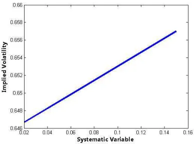
Different starting values of the systematic variable also change the implied volatilities, but in a smoother way, almost imperceptible in figure1. We present in figure2the curve of implicit volatil-ities for different levels ofM0. We fixed Sk0 = 1. The greater the current value of the systematic
Figure 1: Black and Scholes volatility surface
higher levels of the macro variable imply higher risk demanded by investors to compensate for being exposed to the jumps, given that they occur with bigger intensity. The risk of jumps, however, is not captured by the constant volatility of the Black and Scholes model. As a result, extraction of implied volatility results in greater volatility for high levels of jump-risk, that is, high levels of the current systematic variable.
We now proceed to the calculation of the transform that characterizes different derivatives prices.
6
Calculating the discounted characteristic function
In this section, we derive the transform that permits the pricing of derivatives and the computa-tion of other relevant informacomputa-tion, such as the density of the state variables. We won’t be concerned with any specific function, as our immediate goal is only to introduce a parsimonious model capable of extrating the systematic component of the jump-risk premium.
In order to expose the transform, we follow the steps and notation of Duffie, Pan & Singleton
(2000). In their work, they provide a guideline to calculate the price of contigent claims when the state variables have an affine setting, as they have in our model.
For now on, we denote Xtthe vector containing the state variables described in subsection2.2
in the order they have been stated,X0 a given initial condition forXtthat, for simplicity, assures
the mean-reverting processes to start in positive territory, and χ the set of exogenous parameters that determine the dynamics of the model11. Notice that we are dealing with the dynamics under the risk-neutral measure eP. We also denote D ≡ R×R+×R+ ×R+×RN
+ the space on which
the state variables are defined. We want to price an asset that pays the value ea·XT at period T
Figure 2: Black and Scholes volatility curve for fixed strike
contigent on b·XT ≤ y. We compute such price with the function Ga,b(.;X0, T, χ) : R 7→ R+,
which, by risk-neutral pricing is given by:
Ga,b(y;X0, T, χ) =E
exp
− Z T
0
rtdt
ea·XT1b·Xt≤y
Expectations are taken with respect to the same risk-neutral probability that we assume to generate the dynamics described in subsection2.2.
As it is well documented inDuffie, Pan & Singleton(2000), one can use functionGa,b to price
a wide variety of derivatives. An expression for Ga,b can be obtained through the inversion of its
Fourier transform. The Fourier transform, in turn, can be calculated from the discounted conditional characteristic functionψ:C5×D×R+×R+ 7→Cdefined by
ψ(u, Xt, t, T) =E "
exp
− Z T
t
rtdt
eu·XT
Ft
#
Under certain conditions that guarantee that the integrals converge, function ψcan be written in the following way:
ψ(u, s, v, q, r, m1, . . . , mN, t, T) = exp α(u, t, T) +βs(u, t, T)s+βv(u, t, T)v+βq(u, t, T)q
(16)
+βr(u, t, T)r+ N X
i=1
βim(u, t, T)mi !
deal with square root and logarithms of complex numbers, which are not uniquely defined. Our calculations are done according to MatLab (and traditional) standards. For every complex c ∈
C, we define ln(c) = ln|c|+iarg(c) and √c = |c|12 exp
i
arg(c) 2
where arg(c) is defined by c = |c|exp (iarg(c))for−π <arg(c)< π.
For fixedu = (us, uv, uq, ur, um),tandT, the ordinary differential equations (ODE) that these
functions must satisfy are:
˙
βs= 0
˙
βv= −σ 2 v 2
βv2+ [−(ηv−κv)−σvρβs]βv+
˜
µλ1+ 1 2
βs−
βs2
2 −λ1ϕ(β)
˙
βq= " −σ 2 q 2 #
βq2+ [κq]βq+ [βs]
˙
βr= −σ 2 r 2
βr2+ [ζκm]βr+ [1−βs]
˙
βim= −σ 2 im 2
βim2 + [−(ηim−κim)]βim+ [˜µγiβs−γiϕ(β)] fori= 1, . . . , N
where arguments have ommited,β˙ denotes the derivative ofβwith respect to current timet
argu-ment,ϕ(a)≡eµja˜ 1+
a21σ˜ 2
j
2 −1andβdenotes the vector(β
s, βv, βq, βr, β1m, . . . , βN m). The boundary
condition for each of the ODE isβi(u, T, T) =ui withi=s, v, q, r,1m, . . . , N m.
Functionαin turn has to satisfy
˙
α =−λ0ϕ(β) + ˜µλ0βs−κv¯vβv−κqqβ¯ q−κr¯rβr− N X
i=1
κimm¯iβim
with boundary condition α(T) = 0. Once we find βi for i = s, v, q, r, m, we’ll be able to easily
calculate it.
The differential equations relative to the elements of β are of Ricatti type, which in general allows for relatively easy solutions. A deeper look into the equations shows that their solution might be analitically costly since its coefficients are not constant. However, the coefficient depend only onβs, which has a constant solution.
Now we state the solutions. First ODE implies that
βs(u, t, T) =us (17)
For the ODE’s relative toβv,βq,βrandβimfori= 1, . . . , N, general solution can be stated as
βk(u, t, T) = 2dk(u)uk−β¯k(u)
2dk(u) +σk2 uk−β¯k(u) 1−e−dk(u)(T−t) 2dk(u)−
2dk(u) +σ2k uk−β¯k(u)
1−e−dk(u)(T−t) (18)
where we define the following auxiliary functions:
av(u)≡[(ηv−κv) +σvρus] dv(u)≡av(u)2+σv2
(2˜µλ1+ 1)us−us2−2λ1ϕ(u)
1 2
¯
βv(u)≡
dv(u)−av(u)
σ2 v
dq(u)≡ κ2q+ 2σ2qus
1
2 ¯
βq(u)≡ dq(u) +κq
σ2 q
dr(u)≡ kr2+ 2σr2(1−us)
1
2 ¯
βr(u)≡ dr(u) +κr
σ2 r
aim≡ηim−κim dm(u)≡ aim2 + 2σim2 γi(˜µu1−ϕ(u))
1 2
¯
βim(u)≡
dim(u)−aim
σ2im
The last three definitions stand fori= 1, . . . , N.
In the definitions above, theβ¯iterms are particular solutions of the Ricatti differential equations
and can be calculated by solving an ordinary second order polynom. Thedi,av andaimterms are
auxiliary and serve to maintain notation as simple as possible.
We now proceed to the solution of α, which can be found by simple integration of the βi
functions for all thei:
α(u, t, T) =λ0ϕ(u)(T−t)−µλ˜ 0 Z T
t
βsds+κvv¯ Z T
t
βvds+κqq¯ Z T
t
βqds+κrr¯ Z T
t
βrds+ N X
i=1
κimm¯i Z T
t
βmds
Integration of βs is simple. For the other elements of β, integration leads to a function with
the same face since the general solution (18) applies for each one of thoseβi. We define functions
gi(u, t, T)to compute the integrals above:
gk(u, t, T) =−
2dk(u)
σk2 −β¯k
(T−t) (19)
−σ22 k
ln
σ2k
2dk(u) ¯
βk(u)−uk 1−e−dk(u)(T−t)
+e−dk(u)(T−t)
fork=v, q, r,1m, . . . , N m. So finallyαis given by:
α(u, t, T) =λ0(ϕ(u)−µu˜ s) (T −t) +κvv g¯ v(u, t, T) +κqq g¯ q(u, t, T) (20)
+κrr g¯ r(u, t, T) + N X
i=1
κimm¯igim(u, t, T)
finding the solution forGa,bis only a matter of calculating an integral. We shall not go into details,
as the step-by-step has already been documented inDuffie, Pan & Singleton(2000) with a useful example of the process inPan(2002).
What is important for us right now is to highlight once more that through the price of a derivative, we can use observed derivatives prices to extract information on agents perception of a macroeconomic factor.
7
Conclusion
Our goal in this work was to address the question of what factors determine stock jumps. We introduced a model capable of integrating systematic risks into the stock’s risk premia for jumps source of uncertainty. By assuming that the systematic variables influenced the pricing kernel and the jumps intensity, we were able to incorporate them in a classic AJD setting.
While at first sight the systematic variables do not appear to have a very different meaning from idiosyncratic variables, such as volatility, proper application of the model can result into interesting analysis. We proposed an application of the general model to the particular case of macroeconomic variables, or at least variables that we assume agents perceive to be linearly related to the interest rate. In fact, the model can be used to estimate whether agents believe in such relationship.
In the course of this work, we assumed the systematic variables to be driven by uncorrelated Brownian shocks. In many applications, this seems to be a rather strong assumption. In the view of this problem, we also proposed a method to avoid it. Following related literature, the main idea was to work with the shocks in each systematic variable given the realization of the state variables (instantaneous volatility, dividends and interest rate). In order to do that, first we propose a method to extract a volatility series from the data (and this is why we call the whole method a two stage procedure). Although the method leads to a change in the interpretation of some of the coefficients, as it should, by using it we are able to fit a wider class of applications to the framework developed in the baseline model.
References
Andersen, T. G., Fusari, N., & Todorov, V. (2013). Parametric inference and dynamic state recovery from options panels. (Forthcoming in Econometrica).
Ang, A., Piazzesi, M., & Wei, M. (2006). What does the yield curve tell us about gdp growth?
Journal of Econometris,131.
Barigozzi, M., Brownlees, C., Gallo, G. M., & Veredas, D. (2014). Disentangling systematic and idiosyncratic dynamics in panels of volatility measures.Journal of Econometrics,182(2).
Barro, R. (2006). Rare disasters and asset markets in the twentieth century. Quarterly Journal of
Economics,121(3).
Bates, D. S. (1996). Jumps and stochastic volatility: exchange rate processes implicit in deutsche mark options. Review of Financial Studies,9(1).
Bates, D. S. (2000). Post-’87 crash fears in S&P 500 futures options. Journal of Econometrics,94.
Black, F. & Scholes, M. (1973). The pricing of options and corporate liabilities. Journal of Political
Economy,81(3).
Bollerslev, T. & Todorov, V. (2011). Tails, fears and risk premia. Journal of Finance,66.
Bollerslev, T., Todorov, V., & Li, S. Z. (2013). Jump tails, extreme dependencies, and the distribution of stock returns. Journal of Econometrics,172(2).
Broadie, M., Chernov, M., & Johannes, M. (2007). Model specification and risk premia: evidence from futures options. Journal of Finance,62(3).
Chen, R.-R., Liu, B., & Cheng, X. (2010). Princing the term structure of inflation risk premia: theory and evidence from tips. Journal of Empirical Finance,17(4).
Cox, J. C., Ingersoll, J. E., & Ross, S. A. (1985). A theory of the term structure of interest rates.
Econometrica,53(2).
Duffie, D., Pan, J., & Singleton, K. (2000). The transform analysis and asset pricing for affine jump-diffusions. Econometrica,68(6).
Eraker, B., Johannes, M., & Polson, N. (2003). The impact of jumps in volatility and returns.Journal
of Finance,58(3).
Heston, S. L. (1993). A closed-form solution for options with stochastic volatility with applications to bond and currency options. Review of Financial Studies,6(2).
Hinnerich, M. (2008). Inflation-indexed swaps and swaptions. Journal of Banking & Finance,
32(11).
Jarrow, R. & Yildirim, Y. (2003). Pricing treasury inflation protected securities and related deriva-tives using an hjm model. Journal of Financial and Quantitative Analysis,38(2).
Lamoreux, C. G. & Lastrapes, W. D. (1993). Forecasting stock-return variance: toward an under-standing of stochastic implied volatilities. Review of Financial Studies,6(2).
Mehra, R. & Prescott, E. C. (1985). The equity premium: a puzzle. Journal of Monetary Economics,
15.
Pan, J. (2002). The jump-risk premia implicit in options: evidence from an integrated time-series study. Journal of Financial Economics,63.
Piazzesi, M. (2005). Bond yields and the federal reserve. Journal of Political Economy,113(2).