ESCOLA DE P ´
OS-GRADUA ¸
C ˜
AO EM
ECONOMIA
Ot´
avio Menezes Dam´
e
Share Bidding Auctions, Sliding Scale Royalty Rates
and the New Brazilian Regulatory Framework for the
Pre-salt Areas
Share Bidding Auctions, Sliding Scale Royalty Rates
and the New Brazilian Regulatory Framework for the
Pre-salt Areas
Tese para obten¸c˜ao do grau de doutor apre-sentada `a Escola de P´os-Gradua¸c˜ao em Eco-nomia.
´
Area de Concentra¸c˜ao: Teoria Econˆomica
Orientador: Alo´ısio Pessoa de Ara´ujo Coorientador: Paulo Klinger Monteiro
Dam´e, Ot´avio Menezes
Share Bidding Auctions, Sliding Scale Royalty Rates and the New Brazilian Regulatory Framework for the Pre-salt Areas / Ot´avio Menezes Dam´e. – 2014.
52f.
Tese (Doutorado) - Funda¸c˜ao Getulio Vargas, Escola de P´os-Gradua¸c˜ao em Economia.
Orientador: Alo´ısio Pessoa de Ara´ujo. Corientador: Paulo Klinger Monteiro. Inclui Bibliografia.
1. Leil˜oes. 2. Pr´e-sal. 3. Petr´oleo em terras submersas. 4. Informa¸c˜ao assim´etrica. I. Ara´ujo, Alo´ısio Pessoa de, 1946-. II. Monteiro, P. K. (Paulo Klinger). III. Funda¸c˜ao Getulio Vargas. Escola de P´os-Gradua¸c˜ao em Economia. IV. T´ıtulo.
Agradecimentos
Estas ´ultimas linhas que escrevo da tese ser˜ao dedicadas para agradecer aqueles que contribuiram de alguma forma durante o per´ıodo do mestrado e doutorado.
Agrade¸co `a Funda¸c˜ao Getulio Vargas (FGV) pelo apoio institucional; `a Capes, ao CNPq e `a FAPERJ pelo apoio financeiro imprescind´ıvel.
Obrigado ao meu professor orientador, Aloisio Araujo, por toda aten¸c˜ao e dedica¸c˜ao ao longo do mestrado e doutorado. Agrade¸co tamb´em ao professor Paulo Klinger Monteiro pela coorienta¸c˜ao nesta tese e por tudo que aprendi durante esse processo.
Muito obrigado a todos os professores da EPGE pela excelente forma¸c˜ao que re-cebi. Por discuss˜oes e coment´arios relativos `a tese, agrade¸co especialmente os professores Ricardo Cavalcanti, Joisa Saraiva, Moacyr Silva e Luis Braido. Agrade¸co tamb´em aos funcion´ario da escola pelo apoio, em particular `a Marcia Waleria e `a Andrea Machado pela disposi¸c˜ao e presteza que demonstraram sempre que precisei de ajuda.
Agrade¸co ao professor Flavio Cunha pela oportunidade do per´ıodo “sandu´ıche” na University of Pennsylvania. Sempre me recebendo com muita aten¸c˜ao, pude aprender muito durante nossas conversas. Al´em disso, a experiˆencia de estar inserido em uma das melhores universidades do mundo mudou a minha vida.
Devo tamb´em um agradecimento aos meus professores de gradua¸c˜ao Leonardo Mo-nasterio e Nelson Seixas dos Santos. O primeiro foi o respons´avel por despertar meu interesse em economia e o gosto pela pesquisa. O segundo foi a minha inspira¸c˜ao para a carreira em economia, al´em de me dar toda a base para come¸car a sonhar em ingressar na EPGE. Sem eles, eu jamais teria conseguido.
Sou imensamente grato aos meus colegas de mestrado e doutorado por todas as dis-cuss˜oes estimulantes na “pra¸ca”, pelas ajudas quando a tese n˜ao andava e, principalmente, pelos incentivos nos momentos em que o desˆanimo insistia em aparecer. N˜ao posso deixar de mencionar os colegas da turma de 2009 que proporcionaram um ambiente agrad´avel e divertido durante o ´arduo primeiro ano. Na EPGE pude conviver com pessoas sensacio-nais e fazer amigos que levarei sempre comigo. Em especial, agrade¸co aos amigos William Michon Jr. e Cassiano Alves que me acompanharam de perto at´e o fim do doutorado.
Resumo
O governo brasileiro recentemente aprovou uma legisla¸c˜ao instituindo um novo marco regulat´orio para as reservas petrol´ıferas do pr´e-sal. Segundo as novas regras, estas ´areas dever˜ao ser licitadas mediante um leil˜ao de partilha de lucro. Motivado por esta mudan¸ca, apresentamos um modelo de leil˜ao de partilha sob afilia¸c˜ao, demonstrando a existˆencia de um equil´ıbrio mon´otono em estrat´egias puras e caracterizando a solu¸c˜ao. Alem disso, provamos que este mecanismo gera receita esperada maior ou igual a um leil˜ao de primeiro pre¸co usual. Em seguida, introduzimos no modelo uma fun¸c˜ao representando taxas de royalties que dependem do valor do objeto. Este instrumento permite uma eleva¸c˜ao na receita esperada de ambos os modelos, fazendo com que a diferen¸ca entre eles encolha. Finalmente, analisando o novo marco regulat´orio sob o ponto de vista dos resultados obtidos, conclu´ımos que o antigo modelo de concess˜ao utilizado pelo governo brasileiro ´e mais adequado e lucrativo.
Abstract
Brazilian government recently passed legislation instituting a new regulatory framework for the pre-salt reserves. These areas should be negotiated through a profit-share bidding auction. Motivated by this new rules, we present a model of share bidding auction under affiliation, demonstrating the existence of a monotone pure-strategy equilibrium in this structure and characterize its equilibrium bidding function. In addition, we prove that it generates an expected revenue at least as large as the usual fee bidding auction. Next, we introduce in the models a function representing a royalty rate that is contingent to the value of the object. This instrument permits an improvement of expected revenue of both models, making the gap between them shrink. Finally, analyzing this new reg-ulatory framework from the viewpoint of the theoretical and numerical results obtained, we conclude that the former oil regime was more appropriate and lucrative to Brazilian government.
3.1 Expected Revenue and Number of Participants: Param. 1 . . . 22
3.2 Expected Revenue and Number of Participants: Param. 2 . . . 22
3.3 Expected Revenue and Number of Participants: Param. 3 . . . 23
3.4 Expected Revenue and Number of Participants: Param. 4 . . . 23
3.5 Expected Revenue and Number of Participants: Param. 5 . . . 24
4.1 Differences in Expected Revenues for Four Values of σ2 S and v = 1 . . . 29
4.2 Differences in Expected Revenues for Four Values of σS2 and v = 2 . . . 30
4.3 Differences in Expected Revenues for Four Values of σS2 and v = 2.7 . . . . 30
4.4 Differences in Expected Revenues for Three Levels of Variance of C and v = 1 . . . 32
4.5 Differences in Expected Revenues for Three Levels of Variance of C and v = 2 . . . 32
4.6 Differences in Expected Revenues for Three Levels of Variance of C and v = 1 . . . 33
4.7 Differences in Expected Revenues for Three Levels of Variance of C and v = 2 . . . 34
4.8 Differences in Expected Revenues for Three Levels of Variance of C and v at 25% . . . 35
1 Levels of Variance of C for Figures 4.4 and 4.5 . . . 31
2 Levels of Variance of C for Figures 4.6 and 4.7 . . . 33
3 Classification of the Technical Qualification. . . 40
1 Introduction 1
2 The General Model 4
2.1 Share Bidding Auction . . . 5
2.2 Fee Bidding Auction . . . 11
2.3 Ranking of Expected Revenue . . . 13
2.4 Profit-Share and Revenue-Share Bidding Auctions . . . 16
3 Auctions with Sliding Scale Royalty Rates 18 4 Cost Uncertainty 26 5 The New Regulatory Framework for the Brazilian Pre-Salt Fields 37 5.1 Specific Rules for the Auction of the Libra Oil Field . . . 39
5.2 The Results of the First Pre-Salt Round of Bids . . . 42
6 Conclusions 44
References 46
1
Introduction
In 2007, Brazil discovered vast oil reserves in the pre-salt layer, and the country is now poised to become one of the top oil producers in the world. According to estimates from the International Energy Agency (IEA, 2013), the country’s oil production will triple by 2035, turning Brazil into the world’s sixth-largest oil producer. As reported by Petrobras, Brazil’s semi-public multinational energy corporation, oil from the pre-salt layer will account for 52% of total domestic oil production by 2018. The total extent of pre-salt recoverable oil and natural gas is estimated to be around 100 billion barrels of oil equivalent. This discovery tripled the amount of confirmed reserves in the country.
Due to the new discoveries, the Brazilian government recently passed legislation instituting a new regulatory framework for the pre-salt reserves, and one of its components created a system involving a new production sharing agreement. The new rules set forth a profit-share bidding auction, in which the bidding variable is a share of any positive profits earned as a result of winning the project. Therefore, the winner will be the company that offers the largest share of oil output to the government.
All these findings involve large amounts of money and will generate enough wealth to transform Brazil’s economy. Motivated by this new framework, we contribute to the auction literature by rigorously and theoretically studying share bidding auctions and comparing the revenues expected from such auction with fee bidding auctions1. We con-sider a model of interdependent values with n participants where the signals and the common value are affiliated. Under this framework, we demonstrate the existence of a monotone pure-strategy equilibrium in a share bidding auction and characterize its equi-librium bidding function. In addition, we show that this type of auction generates an expected revenue that is at least as large as that generated in a fee bidding auction. The difference in expected revenue can be interpreted as a reduction in the winner’s curse, which allows participants to bid more aggressively.
Following this line of thought, we extend our analysis in section 3 to auctions with sliding scale royalty rates. We introduce a function in the models that represents a royalty rate that is contingent on the value of the object. This instrument permits an improvement in the expected revenue of both models, and causes the gap between them to shrink. With numerical exercises, we show that this result may be caused by a simple sliding scale royalty rates that can easily be implemented in practice. This structure is widely used by governments around the world in auctions for mineral rights.
In section4, we investigate the impact of cost uncertainty on expected revenues. We introduce cost uncertainty because the pre-salt areas require a different technology to be
1
explored, which leads to uncertainty in the costs of production. We propose an auction model in which the object value is known but costs are random and unknown. Under this framework, we examine the impact of high cost uncertainty on expected revenues. The results obtained by numerical methods are dependent on the criteria used to define the cost uncertainty.
Finally, we detail the production sharing agreement adopted by the Brazilian gov-ernment. We discuss Law No. 12351, which has instituted new rules, the tender protocol and the contract for the first and only pre-salt oil field auction thus far. Analyzing this new regulatory framework from the perspective of the theoretical and numerical results obtained in this dissertation, we conclude that the former concession oil regime was more appropriate and lucrative for the Brazilian government.
In the remainder of this section, we briefly review the related literature. We begin withReece(1979), the seminal research that builds uponWilson(1977) andReece(1978) and presents a symmetric, common value auction model with non-negative value and known fixed exploration cost. Using only numerical methods, he studies the expected division of economic rent between participants and auctioneer for profit-share bidding, revenue-share bidding and fee bidding systems. His results show that expected revenues will be highest under profit-share bidding and lowest under fee bidding.
Riley (1988) considers a two-participant common value auction model and shows that if the value of the object is observed ex-post, even if imperfectly, then the seller can increase its expected revenue by adopting a royalty rate bidding auction or requiring that the winning bidder pay a fixed royalty rate in a standard fee bidding system. However, Riley(1988) does not show that the candidate bidding function is, in fact, an equilibrium of the royalty rate bidding auction.
More recently,DeMarzo et al. (2005) andAbhishek et al.(2013) have contributed to this literature. DeMarzo et al.(2005) compare auctions in which the bidding variables are securities whose ultimate values are tied to the resource being auctioned. Their results indicate that expected revenues are positively related to the steepness2 of the securities. It is worth emphasizing that these results are mainly built upon a private value framework. The extension to common value is restricted to a case known as the “wallet game” in which the value of the object equals the sum of the signals observed by the participants. Abhishek et al.(2013) consider a symmetric common value model with a risk neutral auctioneer and either risk averse or risk neutral participants, in a second-price and English auction environments. The first-price auction is not addressed in the paper. These authors divide their model into an auction stage and a profit sharing stage. First, there is a
second-2
price or English auction to choose the winner and determine the initial payment to the seller. The second stage is a profit-sharing contract with a predetermined share fraction. These authors then compare the expected revenue generated by a two-stage model for the case in which there is only the auction stage. They also analyze two types of profit sharing contracts in which either positive profits or both profits and losses are split between the seller and winning buyer. The paper shows that the expected revenue from the model with both types of profit sharing contracts is non-decreasing in the share fraction and higher than the model with only the auction stage. As we discuss in section 3, an excessively high share fraction in our model would discourage the participation of bidders and would lower the expected revenue, which is distinct from their model because they allow negative bids in the auction stage.
2
The General Model
In the economics literature, auctions of mineral rights are typically undertaken by a common value auction model. In this class of model, bidders do not know the real value of the object auctioned until the bidding round is over, but each bidder can observe an estimate or a signal of this value. In mineral rights auctions, the value of the object represents the profit (or the production level) obtained at the end of the project, and the signals correspond to private information or private expectations regarding the project that is the subject of the auction.
We consider a common value auction of a single object withn ≥2 ex-ante identical risk neutral bidders; as used here, the term “ex-ante identical bidders” means that the distributions from which signals are drawn are identical for each bidder. Thus, each bidderi= 1, ..., nobserves a signal3 si, but the value of the object remains unknown until
the auction is over. The common value will be denoted by a real random variable, V. The winner must pay a deterministic costc, which is known to all participants. This deterministic cost may represent a signature bonus, for example. As discussed below in section 5, the signature bonus is a fee paid when the contract for the exploration and production of oil is signed.
Definition 2.1 Let f : A −→ R+, A ⊂ Rn. We say that f satisfies the multivariate monotone likelihood ratio property if∀x, y ∈A,
f(x∨y)f(x∧y)≥f(x)f(y), (2.1)
where(x∨y) = (max{x1, y1}, ...,max{xn, yn})and(x∧y) = (min{x1, y1}, ...,min{xn, yn}).
Next, we discuss the concept of affiliation. The random variables (V, S1..., Sn) are
affiliated if the joint density function f has the multivariate monotone likelihood ratio property. According toMilgrom and Weber(1982a), “this means that a high value of one bidder’s estimate makes high values of the others’ estimates more likely”4, and further-more, the higher the value of v, the higher the probability is of high estimates.
We denote byfthe joint probability density of then+1 real valued random variables V, S1, ...Sn.
Assumption 2.1 f(s1, ..., sn, v) = h(v)g(s1, v). . . g(sn, v) and
R
g(z, v)dz = 1, ∀v ∈
supp(V).
Assumption 2.1 implies that each signal is conditionally independent of the others, 3
This signal is also called an informational variable or value estimate.
4
given V =v, i. e., f(s1, ..., sn, v) =h(v)g(s1|v). . . g(sn|v). In other words, given the real
value of the object, the estimates of the participants are independent.
Assumption 2.2 Density function g satisfies the monotone likelihood ratio property.
Assumption 2.2 entails that the bidders’ estimates and the value of the object are affiliated, i.e., f is affiliated. This assumption matches well with an oil leasing auction and is commonly used in the literature because the estimates obtained by oil companies are higher when the quantity of recoverable oil in the field is larger.
The following lemmas are required for the proofs presented in this section.
Lemma 2.1 LetΦ1,Φ2,Φ3, andΦ4 denote non-negative functions on Rn such that for all
x, y ∈Rn,Φ
1(x)Φ2(y)≤Φ3(x∨y)Φ4(x∧y). Then,
R
Φ1(x)dx
R
Φ2(x)dx≤
R
Φ3(x)dx
R
Φ4(x)dx
Proof: Menezes and Monteiro (2005, pp. 62, 168-169).
Lemma 2.2 Let Z1, ..., Zk be affiliated, and let H be any increasing function. Then, the function h defined by
h(a1, b1, ..., ak, bk) = E[H(Z1, ..., Zk)|a1 ≤Z1 ≤b1, ..., ak≤Z1 ≤bk]
is increasing in all its arguments. In particular, the functions
hl(z1, ..., zl) =E[H(Z1, ..., Zk)|z1, ..., zl]
for l= 1, ..., k are non-decreasing.
Proof: Karlin and Rinott(1980, pp. 484) and Sarkar (1969).
Lemma 2.3 The function G(x,v)g(x,v) is non-decreasing in v.
Proof: By the affiliation inequality, for any α ≤ x and any v′ ≤ v′′, we must have g(x, v′′)g(α, v′) ≥ g(α, v′′)g(x, v′). Thus, Rx
−∞g(x, v′′)g(α, v′)dα ≥ Rx
−∞g(α, v′′)g(x, v′)dα implies the result.
2.1
Share Bidding Auction
of the revenue generated as a result of winning the auction. As we discuss further below, the model presented here is general enough to fit both profit-sharing and revenue-sharing bidding auctions.
In the following cases, we look for a symmetric, continuous and strictly increasing equilibrium bidding function5 b : S
i → [0,1]. In a symmetric bidding environment, it is
possible to take the perspective of bidder 1 in the game without any loss of generality. Thus, we consider the problem faced by bidder 1. and we denote by Y1 the random
variable of the largest realization of the signal among{S2, ..., Sn}. The subscript sstands
for the share bidding auction. We assume that other participants use the equilibrium strategyb∗s(·). Letx+≡max{x,0}, andx− ≡max{−x,0}. The expected payoff of player 1 given that he observes signalsand bids as if he had observed signal xis represented by the function below:
ψs(x) =E
(V −b∗(x)V+−c)I{b∗(Y1)<b∗(x)}|S1 =s
. (2.2)
Thus, we search for the bidding function bs(·) that maximizes expression (2.2).
We must satisfy the participation constraint: ψs(x)≥0. Otherwise, bidder 1 would do better by bidding zero rather than receiving negative expected payoff. We define s∗s as the highest value ofx such that bidder 1 would rather bid zero than a positive share. Thus, s∗
s is defined such thatψs(s∗s) = 0 and b∗s(s∗s) = 0. In equilibrium, x=s, so bidders choose not to participate ifs < s∗
s.
For the next theorem, we define ˆf(s, y) = R
h(v)g(s, v)(n−1)Gn−2(y, v)g(y, v)dv,
whereG(s, v) = R
z<sg(z, v)dz.
Theorem 2.1 The bidding function b∗s is a symmetric equilibrium of the share bidding auction such that:
b∗s(s) = Z s
s∗
s e−R
s
t Ds(z)dzAs(t)dt (2.3)
where
As(s) = R
(v−c)h(v)g(s, v)(n−1)Gn−2(s, v)dv
R
v+h(v)g(s, v)Gn−1(s, v)dv ,
Ds(s) = R
v+h(v)g(s, v)(n−1)Gn−2(s, v)dv
R
v+h(v)g(s, v)Gn−1(s, v)dv .
(2.4)
5
Moreover, b∗
s solves
b∗′s(s) =As(s)−b∗s(s)Ds(s);
b∗s(s∗s) = 0. (2.5)
Proof: To ease notation, we will suppress subscripts. Note that
ˆ
f(s, y) = Z
h(v)g(s, v)(n−1)Gn−2(y, v)g(y, v)dv= Z
h(v)g(s, v)H′(y, v)dv (2.6)
whereH(y, v) = Gn−1(y, v). Define Y = max{sj :j 6= 1}, and
u+(s, y) = E
V+|S1 =s, Y =y
=
Z
vI{V≥0}
h(v)g(s, v)H′(y, v) ˆ
f(s, y) dv
u−(s, y) = EV−|S1 =s, Y =y
=
Z
−vI{V <0}
h(v)g(s, v)H′(y, v) ˆ
f(s, y) dv.
(2.7)
It is worth highlighting thatu+(s, y)−u−(s, y) =u(s, y). Consider bidder 1’s expected payoff:
ψ(x) =E(V −b(x)V+−c)I{b∗(Y1)<b(x)}|S1 =s
=
E
E
((1−b(x))V+−V−−c)I{Y1<x}|S1, Y1
|S1 =s =
E(1−b(x))u+(S1, Y1)I{Y1<x}|S1 =s
−E(u−(S1, Y1) +c)I{Y1<x}|S1 =s
= (1−b(x))
Z x
−∞
u+(s, y) ˆf(s, y)dy−
Z x
−∞
u−(s, y) ˆf(s, y)dy−c Z x
−∞ ˆ
f(s, y)dy. (2.8)
Deriving ψ(x), we have
ψ′(x) =−b′(x) Z x
−∞
u+(s, y) ˆf(s, y)dy+(1−b(x))u+(s, x) ˆf(s, x)−u−(s, x) ˆf(s, x)−cf(s, x).ˆ (2.9)
If b∗ is a best reply for 1, we must have ψ′(x) = 0 when x=s. Then,
b∗′(x) = [(1−b∗(x))u
+(x, x)−u−(x, x)−c] ˆf(x, x) Rx
−∞u+(x, y) ˆf(x, y)dy
If we substitute equation (2.10) in (2.9), we have,
ψ′(x) =− [(1−b(x))u
+(x, x)−u−(x, x)−c] ˆf(x, x) Rx
−∞u+(x, y) ˆf(x, y)dy
Z x
−∞
u+(s, y) ˆf(s, y)dy+
+
(1−b(x))u+(s, x)−u−(s, x)−c ˆ f(s, x)
(2.11)
We must show that b∗ is an optimal bidding function. It is sufficient to prove that ψ′(x)≥ 0 when x < s and ψ′(x) ≤ 0 when x > s. Hence, assume that x < s. We have ψ′(x)≥0 if and only if
(1−b(x))u+(s, x)−u−(s, x)−c≥
(1−b(x))u+(x, x)−u−(x, x)−c f(x, x)ˆ Rx
−∞u
+(s, y) ˆf(s, y)dy
ˆ
f(s, x)Rx
−∞u+(x, y) ˆf(x, y)dy (2.12)
Thus, if we have
1≥
ˆ
f(x, x)Rx −∞u
+(s, y) ˆf(s, y)dy
ˆ
f(s, x)Rx
−∞u+(x, y) ˆf(x, y)dy
(2.13)
the inequality (2.12) holds, because (1−b(x))u+(s, x)≥(1−b(x))u+(x, x) andu−(s, x)≤ u−(x, x). However, if we assume
1< ˆ
f(x, x)Rx −∞u
+(s, y) ˆf(s, y)dy
ˆ
f(s, x)Rx
−∞u+(x, y) ˆf(x, y)dy
(2.14)
it is enough to show that
u−(s, x) ˆf(s, x)−u−(x, x) ˆf(x, x) Rx
−∞u+(s, y) ˆf(s, y)dy Rx
−∞u+(x, y) ˆf(x, y)dy
≤0 (2.15)
and
u+(s, x) ˆf(s, x)−u+(x, x) ˆf(x, x) Rx
−∞u
+(s, y) ˆf(s, y)dy
Rx
−∞u+(x, y) ˆf(x, y)dy
because
(1−b) "
u+(s, x) ˆf(s, x)−u+(x, x) ˆf(x, x) Rx
−∞u+(s, y) ˆf(s, y)dy Rx
−∞u+(x, y) ˆf(x, y)dy #
≥0≥
≥c "
ˆ
f(s, x)− ˆ
f(x, x)Rx −∞u
+(s, y) ˆf(s, y)dy
Rx
−∞u+(x, y) ˆf(x, y)dy #
+
+ "
u−(s, x) ˆf(s, x)−u−(x, x) ˆf(x, x) Rx
−∞u
+(s, y) ˆf(s, y)dy
Rx
−∞u+(x, y) ˆf(x, y)dy #
(2.17)
We begin by expression (2.15). Note thatu−(s, x) = E[V−|s, x] =E
−V I{v<0}|s, x
=
−EV I{v<0}|s, x
. Then, by Lemma2.2, we know that u−(s, x) is non-increasing ins and x. Thus,
0≥u−(x, x) "
ˆ
f(s, x)−fˆ(x, x) Rx
−∞u
+(s, y) ˆf(s, y)dy
Rx
−∞u+(x, y) ˆf(x, y)dy #
=
= "
u−(x, x) ˆf(s, x)−u−(x, x) ˆf(x, x) Rx
−∞u+(s, y) ˆf(s, y)dy Rx
−∞u+(x, y) ˆf(x, y)dy #
≥
≥
"
u−(s, x) ˆf(s, x)−u−(x, x) ˆf(x, x) Rx
−∞u
+(s, y) ˆf(s, y)dy
Rx
−∞u+(x, y) ˆf(x, y)dy #
(2.18)
Now, we show expression (2.16) is valid. Note that
u+(s, x) ˆf(s, x) = Z
v+h(v)g(s, v)H′(x, v)dv (2.19)
u+(x, x) ˆf(x, x) = Z
v+h(v)g(x, v)H′(x, v)dv (2.20) Z x
−∞
u+(s, y) ˆf(s, y)dy= Z
v+h(v)g(s, v)H(x, v)dv (2.21)
Z x
−∞
u+(x, y) ˆf(x, y)dy = Z
v+h(v)g(x, v)H(x, v)dv (2.22)
Substituting the equations above into the inequality (2.16), we must prove that
Z
v+h(v)g(s, v)H′(x, v)dv·
Z
v+h(v)g(x, v)H(x, v)dv≥
Z
v+h(v)g(x, v)H′(x, v)dv· Z
v+h(v)g(s, v)H(x, v)dv
We now choose (
Φ4(s, v) = Φ2(s, v) = v+h(v)g(s, v)H(x, v)
Φ3(s, v) = Φ1(s, v) = v+h(v)g(s, v)H′(x, v)
(2.24)
Thus,
Φ3(s′ ∨s′′, v′ ∨v′′)Φ4(s′∧s′′, v′∧v′′)≥Φ1(s′, v′)Φ2(s′′, v′′) (2.25)
if and only if,
g(s′∨s′′, v′∨v′′)g(s′ ∧s′′, v′∧v′′)H′(x, v′∨v′′)H(x, v′∧v′′)≥
g(s′, v′)g(s′′, v′′)H′(x, v′)H(x, v′′) (2.26)
As g(s′ ∨s′′, v′ ∨v′′)g(s′ ∧s′′, v′ ∧v′′) ≥ g(s′, v′)g(s′′, v′′) is satisfied, we must only check that
(n−1)Gn−2(x, v′∨v′′)g(x, v′∨v′′)Gn−1(x, v′∧v′′) = H′(x, v′∨v′′)H(x, v′∧v′′)≥ H′(x, v′)H(x, v′′) = (n−1)Gn−2(x, v′)g(x, v′)Gn−1(x, v′′)
(2.27)
Dividing both sides of the inequality by (n−1)Gn−2(x, v′∨v′′)g(x, v′∨v′′)Gn−2(x, v′∧ v′′), we have
g(x, v′∨v′′)G(x, v′∧v′′)≥g(x, v′)G(x, v′′). (2.28)
If v′ ≥ v′′, we have the equality in (2.28). If v′ < v′′, by Lemma 2.3 we have
g(x,v′′)
G(x,v′′) ≥
g(x,v′)
G(x,v′). Thus,
g(x, v′∨v′′)G(x, v′∧v′′) =g(x, v′′)G(x, v′)≥g(x, v′)G(x, v′′). (2.29)
Thus, as expression (2.25) is satisfied, using Lemma 2.1 we must have
Z
Φ3(x∨s, v)dv
Z
Φ4(x∧s, v)dv≥
Z
Φ1(x, v)dv
Z
Φ2(s, v)dv. (2.30)
Finally, we conclude that ψ′(x)≥0. If x > s, the proof is analogous.
b∗′(s) =A(s)−b∗(s)D(s). (2.31)
We solve the differential equation using the integrating factor method. Considering the initial conditionb∗(s∗) = 0, we have equation (2.3).
We have to check that b∗ is increasing. In this regard, first we will show that the ratio A(x)D(x) <1 is increasing. Since v−c=v+−(v−+c) ≤ v+ it is immediate A(s)
D(s) <1.
We may write
A(s) D(s) =
R
(v−c)g(s, v)H′(s, v)h(v)dv R
v+g(s, v)H′(s, v)h(v)dv = 1− R
(v−+c)g(s, v)H′(s, v)h(v)dv R
v+g(s, v)H′(s, v)h(v)dv .
Thus it suffices to prove that
R
(v−+c)g(s,v)H′(s,v)h(v)dv
R
v+g(s,v)H′(s,v)h(v)dv is decreasing. Note that
R
(v−+c)g(s, v)H′(s, v)h(v)dv R
v+g(s, v)H′(s, v)h(v)dv =
E[V−+c|S
1 =s, Y =s]
E[V+|S
1 =s, Y =s]
.
Lemma2.2 implies that the denominator is increasing and the numerator is decreasing. We will prove that b∗′(s)>0. For this it suffices to prove that b∗(s)< A(s)
D(s). Thus
b∗(s) = Z s
s∗
e−RtsD(z)dzA(t)dt=
Z s
s∗
e−RtsD(z)dzA(t)
D(t)D(t)dt
≤ DA(s)
(s) Z s
s∗
e−RtsD(z)dzD(t)dt = A(s)
D(s)
e−RtsD(z)dz
|s s∗ =
= A(s) D(s)
1−e−Rss∗D(z)dz
< A(s) D(s).
So, the bidding functionb∗(·) is strictly increasing and smaller than 1.
Thus, we demonstrate that the differential equation resulting from the first-order condition is the equilibrium function of the auction.
2.2
Fee Bidding Auction
We now define the usual fee bidding auction following Milgrom and Weber (1982a). With this model, we can establish a ranking of expected revenue, and in the following sections, we use this ranking as a benchmark for other models.
In this model, the winner is the bidder who offers the highest fee. The subscript f
fee, and not a share of the object as in the previous model. The expected payoff of player 1 that observes signal s and bids as if the signal observed is x is given by the following expression:
ψf(x) = E
h
(V −b∗f(x)−c)I{b∗
f(Y1)<b∗f(x)}|S1 =s i
. (2.32)
We must define s∗f in the same manner as we did for the share bidding auction. Thus, s∗f is defined such that ψf(s∗
f) = 0 and b∗f(s∗f) =u(0,0)−c= 0, and bidders decide not to participate if x < s∗f.
The cost c is also present here such that we can make a fair comparison with the share bidding model. Although not as common as in this type of auction, c may stand for a signature bonus or any other predetermined fee that the winning bidder must pay to the auctioneer.
Next, we reproduce a theorem from Milgrom and Weber (1982a) that characterizes the equilibrium bidding function of the fee bidding auction. The proof for this theorem appears in appendix A.
Theorem 2.2 (Milgrom and Weber, 1982a) The bidding function b∗
f is an equilibrium of the fee bidding auction such that:
b∗f(x) = Z s
s∗
e−RtsDs(z)dzAs(t)dt. (2.33)
where
Af(s) = R
(v−c)h(v)g(s, v)(n−1)Gn−2(s, v)dv
R
h(v)g(s, v)Gn−1(s, v)dv ,
Df(s) = R
h(v)g(s, v)(n−1)Gn−2(s, v)dv
R
h(v)g(s, v)Gn−1(s, v)dv .
(2.34)
Moreover, b∗f solves
b∗′f (s) =Af(s)−b∗f(s)Df(s);
b∗f(s∗) = 0. (2.35)
2.3
Ranking of Expected Revenue
In light of both auctions previously examined, we now present a theorem of expected revenue ranking. Our main finding is that, under the assumption that signals are affiliated, the share bidding auction outperforms the fee bidding auction. The reasons underlying this result are explored and discussed throughout this section.
Assume that all bidders follow the symmetric equilibrium strategies previously dis-cussed. LetQa(s, x) be the expected value paid by the winner in an auctiona given that he observed signals but bid as if he had observed signalx.
When declared the winner of a fee bidding auction, bidder 1 will pay exactly his own bid plus the cost, c. Thus,
Qf(s, x) =b∗f(x) +c,
where b∗f(·) is the symmetric equilibrium strategy that is characterized by expression (2.33).
In a share-bidding auction, the expected value paid by the winner depends on the value of the object. Then, the amount he will have to pay if he is the winning bidder will be expressed in terms of the expectation of V. Hence, the expected payment upon winning is given by
Qs(s, x) = b∗s(x)E[V|S1 =s, Y1 < x] +c
We denote the partial derivative ofQawith respect to its first argument byQ
(1)
a (·,·). We use the following result from Krishna (2010) to demonstrate the revenue ranking of the models.
Theorem 2.3 Krishna (2010, Proposition 7.1) Let a and b be two auctions in which the highest bidder wins and only he pays a positive amount. Suppose that each has a symmetric and increasing equilibrium such that
(i) for all s, Q(1)a (s, s)≥Q(1)b (s, s); (ii) Qa(s∗, s∗) = 0 =Qb(s∗, s∗).
Then, the expected revenue in auction a is at least as large as in b.
Proof: AppendixA.
assume the same value of cost cfor both models.
Corollary 2.1 The expected revenue from a share bidding auction is at least as large as the expected revenue from the fee bidding auction.
Proof: Observe that Q(1)f (s, s) = 0, as Qf(s, x) = b∗
f(x) + c does not depend on s. However, note that Q(1)s (s, s) ≥ 0. This result follows immediately from Lemma 2.2. Thus, we conclude that expected revenue from the share bidding auction is at least as large as the expected revenue from the fee bidding auction.
All these results lead us to the Linkage Principle, stated by Milgrom and Weber (1982a). According to the Linkage Principle, open auctions will generate higher expected revenues than sealed-bid auctions. Under affiliation assumption, Milgrom and Weber (1982a) establish a revenue ranking of auctions: English ≥ second-price≥ first-price. In the first-price auction, there is no linkage between the bidders, whereas the expected win-ning bid of second-price auction also depends on the signal observed by the second highest bidder. Finally, in the English auction, the expected price depends on the information of all the bidders. Therefore, a stronger linkage results in an increase in the expected value of the good to a bidder that is conditional on observing the highest signal. Thus, bidders will bid more aggressively and generate higher than expected revenue.
According to de Castro (2010), we should be careful when interpreting the Linkage Principle. Frequently, the intuitions6 consider the notion of positive dependence of the signals and the common value, but it can be formalized in several diffent ways. In this paper, de Castro describes seven different formal concepts of positive dependence for random variables and shows that affiliation is the strongest one. Hence, the author shows that the result of revenue ranking ofMilgrom and Weber (1982a) is not robust for other definitions of positive dependence. So, an intuition for this result based only in positive dependence of the random variables may be inaccurate.
Due to this fact, we concentrate our interpretation in a particular case. Consider the following assumption and lemma:
Assumption 2.3 The return V has a normal distribution, N(µ, σ2
V). The signal Si,
i = 1, . . . , N conditional on V is normally distributed with mean V and variance σ2.
6
Thus
f(s1, . . . , sN, v) =h(v)g(s1|v)· · ·g(sN|v),
h(v) = 1 σV
√
2πexp −
(v−µ)2 2σ2
V
! ,
g(si|v) =
1
σ√2πexp −
(si−v)2
2σ2
! .
Lemma 2.4 The densityf has multivariate monotone likelihood ratio.
Proof: It suffices to show that g(s|v) = 1 σ√2π exp
−(s2σ−v)22
has monotone likelihood ratio. This is true, since if s′′ > s′,
g(s′′|v) g(s′|v) =
1 σ√2πe
−(s′′−v)
2
2σ2
1 σ√2πe
−(s′−v)
2
2σ2
=e(
s′−v)2 2σ2 −
(s′′−v)2
2σ2 = exp
(s′′−s′) (2v −s′−s′′) 2σ2
is increasing in v.
According to lemma 2.4, the conditional independence of the signals implies affilia-tion under a normal distribuaffilia-tion. In the following interpretaaffilia-tion, we only use the property of conditional independence of the signals. First, we introduce the phenomenon of the winner’s curse. The winner of a common value auction is the one with the most optimistic estimate of the object’s value. If we assume that the average bid is accurate, then winning bids will probably exceed the true value of the good. Thus, under rationality assumption, bidders will recognize that winning is informative about being potentially overoptimistic and will bid less aggressively.
If the winner’s payment is contingent on the ex-post value of the good, the threat of the winner’s curse is not as severe. Overestimating the share bidding auction means that the bidder will pay a higher share than he would be willing to pay if he knew the true value of the object. Thus, the lower the true value of the good is, the lower the winner’s total payment, which is unlike the result in the fee bidding auction because total payment does not depend on the true value of the good. Winning a share bidding auction is not as bad news as winning a fee bidding auction, so bidders can be more aggressive.
an alternative model that is already used worldwide.
2.4
Profit-Share and Revenue-Share Bidding Auctions
The two most common bidding variables in a share bidding auction are the share of profit and the share of revenue, specially for oil and gas lease auctions. As the name suggests, the revenue-share bidding model assumes that the bidding variable is a fraction of the revenue earned by the winner. However, in the profit-share bidding model, the bidding variable is a fraction of any positive profits earned as a result of winning the auction. Thus, the main difference between these two approaches is that shares will be calculated after deducting exploration and production costs in an oil lease profit-share auction.
Despite the similarity between the profit-share and revenue-share auctions, they may generate substantially different expected revenues for the auctioneer. Using numerical methods,Reece(1979) shows that profit-share bidding auctions generate higher expected revenue than revenue-share bidding auctions.
Our share-bidding model covers both profit-share and revenue-share bidding for-mulations from Reece (1979), who presents a model with common, unknown, and non-negative values and with known fixed costs. We can fit both structures only by making assumptions about the random variable V, which should be understood as the project revenue auctioned, and by looking at c as the fixed costs. If we then assume that V is non-negative, we are in Reece’s revenue-share bidding structure. TakingV as non-negative and shifted to the left, i.e., considering the expected payoff
E(W −b(x)W+)I{b∗(Y1)<b(x)}|S1 =s
,
whereW =V −c, we mimic Reece’s profit-share bidding formulation.
Considering an oil leasing auction, there may be a principal-agent problem in the profit-share formulation that does not affect the revenue-share model. From the govern-ment’s perspective, it is much easier to identify the amount of extracted oil than to verify all the production and exploration costs. In a profit-share contract, the winning firm would have incentives to misreport costs and keep a larger profit share by so doing. Thus, the government would have to use some monitoring system to avoid this type of problem.7 Assume that there is a technology that the government can use to observe all the exploration costs perfectly by paying a given fixed monitoring cost. Assuming that the government will use this technology, then corollary 2.1 may not hold anymore, i.e., a
7
3
Auctions with Sliding Scale Royalty Rates
In this section, we consider an auction in which the winner will be required to pay a pre-fixed sliding scale royalty rate (SSRR) that is based on the value of the good, in addition to the bid amount (a fee or a share, depending on which auction is being considered). We show that this rule may increase the expected revenue of both models studied in the previous section and shrink the gap between them.
This type of rule is frequently used in oil lease auctions around the world. Govern-ments set up some ranges of revenue or production volume and determine extra royalty rates to be paid when these ranges are reached. The SSRR is frequently based on the av-erage daily production per well per month in a given area. In most cases, the international price of oil is also consider in the SSRR arrangement.
In the model developed in this section, we depict the SSRR by a function that depends on v. The random variable V represents a monetary value, which means that it responds to the productivity and total value of the auctioned oil field. Thus, defining the SSRR over v is a good way to represent the real world. Let ξ : R+ −→ R+ be the
function representing the SSRR.
Assumption 3.1 The function ξ(·) is continuous, increasing and such that t7→t−ξ(t) is increasing and ξ(0) = 0.
According to assumption 3.1, as the value of the object rises, the bidder’s payoff should also rise. An increasing bidding function only makes sense when the bidder’s payoff increases when the signal observed is higher. Without this assumption, we would not be able to find a strictly increasing bidding function.
In both models, the function ξ is defined only on the positive part ofV. We make this assumption to exclude the possibility of royalties being paid when the object’s value is negative. The subscripts ¯f and ¯s stand for the fee and share bidding auctions with SSRR, respectively.
Now, we define a fee bidding auction with SSRR. Again, we analyze the model from bidder 1’s perspective. Assuming that other participants use the equilibrium strategyb∗
¯f,
bidder 1’s problem is to maximize the following expression:
ψ¯f(x) = E
(V −b¯∗f(x)−ξ(V+))In
b∗
¯f(Y1)<b¯∗f(x)
o|S
1 =s
. (3.1)
Next, we define a share bidding auction with SSRR. Assume that bidder 1’s problem is expressed by the following equation:
ψ¯s(x) =E (1−b¯s∗(x))(V+−ξ(V+))−V−
I{b∗ ¯
s(Y1)<b∗¯s(x)}|S1 =s
. (3.2)
In the share bidding auction, the implementation of an SSRR deserves more atten-tion. Equation (3.2) shows that the royalty rates are first subtracted from the value of v, and then, the winner’s bid is deduced from this amount. This form facilitates the demon-stration of the existence of and the characterization of the equilibrium bidding strategy of this auction.
The initial conditions s∗
¯f and s∗¯s are defined in a similar way to section 2. The following corollaries present the solution for the fee bidding auction with SSRR and for the share bidding auction with SSRR:
Corollary 3.1 The bidding function b¯∗f is an equilibrium of the fee bidding auction with SSRR such that:
b¯∗f(x) =
Z s
s∗
e−RtsD¯f(z)dzA¯
f(t)dt., (3.3)
where
A¯f(s) =
R
(v−ξ(v))h(v)g(s, v)(n−1)Gn−2(s, v)dv
R
h(v)g(s, v)Gn−1(s, v)dv ,
D¯f(s) =
R
h(v)g(s, v)(n−1)Gn−2(s, v)dv
R
h(v)g(s, v)Gn−1(s, v)dv .
(3.4)
Moreover, b¯∗f solves
b¯∗′f (s) =A¯f(s)−b¯∗f(s)D¯f(s);
b¯∗f(s¯∗f) = 0.
(3.5)
Corollary 3.2 The bidding function b∗
¯s is an equilibrium of the share bidding auction with SSRR such that:
b¯∗s(s) = Z s
s∗
where
A¯s(s) =
R
(v−ξ(v+))h(v)g(s, v)(n−1)Gn−2(s, v)dv
R
v+h(v)g(s, v)Gn−1(s, v)dv ,
D¯s(s) =
R
(v+−ξ(v+))h(v)g(s, v)(n−1)Gn−2(s, v)dv
R
v+h(v)g(s, v)Gn−1(s, v)dv .
(3.7)
Moreover, b∗¯s solves
b¯∗′s(s) =A¯s(s)−b¯∗s(s)D¯s(s); b¯∗s(s∗
¯
s) = 0.
(3.8)
Note that E[V −ξ(V+)|S
1 =s, Y =y] and E[V+−ξ(V+)|S1 =s, Y =y] are
non-decreasing in s and y because of assumption 3.1. Thus, the proof of corollaries 3.2 and 3.1 follow from the theorems2.1 and 2.2, respectively.8
From this equilibrium result, we would like to show that it is possible to improve the expected revenue by introducing an SSRR into the model. It is not simple to reach this result analytically because an aggressive royalty rate may result in the opposite effect. The main difficulty is to determine a shape of the functionξthat would lead to an increase in the expected revenue. Thus, the problem will be illustrated by numerical methods, and we select examples of some SSRRs to verify the expected revenue changes.
Because numerical methods will be used, we consider assumption 2.3 and lemma 2.4. We assumeV with variance σV2 = 100. The meanµV is set such that approximately
25% of all oil fields are economically viable (µV ∼=−2.133). We assume that the signals
are unbiased; in other words, we assume that the distribution of the signalSi is set in such
a way thatE[Si|v] =v. In addition, the random variable S|v is assumed to be normally
distributed with mean v and variance σ2 = 49. We are considering a symmetric model,
so all agents observe signals from the same distribution.
Based on the parameter values, we look into some examples of SSRRs that permit us to identify the results we want to show. We divide the support ofV+ into k intervals
8
and defineξ(·) as: ξ(v) =
0 if v < v1
δ1(v−v1) if v ∈[v1, v2)
δ1(v2−v1) +δ2(v−v2) if v ∈[v2, v3)
...
k−2
P
i=1
δi(vi+1−vi) +δk−1(v −vk−1) ifv ≥vk−1.
(3.9)
Let V = [v1 v2 v3 . . . vk−1] and ∆ = [δ1 δ2 δ3 . . . δk−1]. We assign different values
to these vectors, which makes the SSRR more or less aggressive depending on the level of the royalty rates (∆) and the thresholds (V). Thus, when rate levels are higher and thresholds are lower, the SSRR is more aggressive.
According to the function ξ described above, the royalty rates are calculated sepa-rately in each interval. For example, assume thatV = [2 3 4 5] and ∆ = [0.2 0.3 0.4 0.5]. If the realization of the common value isv = 4.5, the amount of royalty due to the auc-tioneer will beξ(4.5) = 0.2(3−2) + 0.3(4−3) + 0.4(4.5−4) = 0.7. Assuming that ˜b¯f and ˜b¯s are the winning bids of the fee and share bidding models respectively, the amount of the final payoffs of the winner will be
P O¯f=v−˜b¯f−ξ(v) = 4.5−˜b¯f−0.7 = 3.8−˜b¯f;
P O¯s = (1−˜bs)(v¯ −ξ(v)) = (1−˜b¯s)(3.8).
Next, we present five parameterizations that go from less to more aggressive SSRRs:
• Parametrization 1: V = [2 3 4 5] and ∆ = [0.2 0.3 0.4 0.5];
• Parametrization 2: V = [1 1.5 1.8 2.2] and ∆ = [0.2 0.3 0.4 0.5];
• Parametrization 3: V = [1 1.5 1.8 2.2] and ∆ = [0.4 0.6 0.7 0.9];
• Parametrization 4: V = [1 1.5 1.8 2.2] and ∆ = [0.96 0.97 0.98 0.99];
• Parametrization 5: V = [0.1 0.3 0.5 0.7] and ∆ = [0.96 0.97 0.98 0.99].
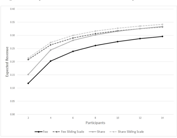
Figure 3.1: Expected Revenue and Number of Participants: Param. 1
Figure 3.3: Expected Revenue and Number of Participants: Param. 3
Figure 3.4: Expected Revenue and Number of Participants: Param. 4
are implemented in the model. Moreover, the gap between the dashed lines is narrowing and practically disappears in the last figure.
When an SSRR is present in an auction, the winner’s final payment becomes more connected to the value of the object. In the case of overestimation, the punishment of the winning bidder is less severe compared with the standard auctions, which means that the effects of the winner’s curse will be ameliorated and, as a consequence, bidders will be more comfortable to bid more aggressively. Thus, the SSRR allows the seller to capture a larger share of the bidders’ surplus.
Figure 3.5: Expected Revenue and Number of Participants: Param. 5
However, if the SSRR is too aggressive, bidders will require a very high signal to begin bidding, and the auctioneer’s expected revenue may fall short. On these terms, bidders’ expected payoff for a large set of observed signals s will be so small that they will prefer to sit out the auction. In other words, the value ofs∗ will be very high, which is what occurred in the exercise presented in Figure3.5.
exercise depicted in Figure3.5 did not decrease the expected revenue when only two par-ticipants were competing for the object. Hence, the optimal functionξ, if it really exists, will surely depend on the level of competition in the auction.
Although we do not have a result that characterizes the optimal function ξ, the numerical exercises presented here have shown that there is no need for complex functions to reach the desired results. With SSRRs that could easily be implemented in a real case, our models generate higher expected revenue and almost eliminate the gap between the fee and share bidding auctions.
Results also indicate that more competition tends to increase the expected revenue. In particular cases, an additional bidder increases the expected revenue almost as much as the adoption of a new mechanism for the auction.9
9
Bulow and Klemperer(1996) compare the expected revenue improvement of drawing more partici-pants and of choosing the design of the auction. With independent signals and risk-neutral bidders, the authors show that an usual english auction withn+ 1 bidders generates higher expected revenue than
4
Cost Uncertainty
Brazil’s pre-salt reserves are deeply buried beneath two kilometers of water, a layer of rocks and up to two kilometers of shifting salt. By reason of its geological features, the pre-salt layer requires technology to be employed that is more resistant both to corrosion and to high temperatures and pressure. Therefore, there is substantial uncertainty regarding the cost of meeting the technical challenges of developing the pre-salt layer.
The objective here is to investigate how the gap between the expected revenues from the profit-share and revenue-share bidding auctions respond to changes in the cost variance. To conduct such investigation, we will employ a model in which the value of the object is known by all the bidders, but the associated costs are unknown. Therefore, the unknown cost will be denoted by the random variableC, whereas the constantv will represent the value of the object. The signal si observed by bidder i is related to the
unknown costC; thus, the equilibrium will be characterized by decreasing functions. The assumptions for the random variables are analogous to those we have made in section 2.
LetG(x, c) =R
y<xg(y, c)dy and
˜
f(s, y) = Z
h(c)g(s, c)(n−1) [1−G(y, c)]n−2g(y, c)dc= Z
h(c)g(s, c)H′(y, c)dc (4.1)
whereH(y, c) = 1−[1−G(y, c)]n−1. Define Z = min{Sj :j 6= 1}.
First, we define the revenue-share bidding auction. Again, we picture the problem faced by bidder 1. Given that he observes signals and bids as if he had observed signal x, the expected payoff of bidder 1 is:
ψrs(x) = E((1−b∗rs(x))v−C)I{b∗
rs(Z)<b∗rs(x)}|S1 =s
(4.2)
With decreasing bidding functions, we will have a maximum value of the signal such that bidders choose not to participate if a higher s is observed. Thus, s∗
rs is defined such thatψrs(s∗rs) = 0 andb∗rs(s∗rs) = 0. In addition, bidders do not participate in the auction if s > s∗rs.
Thus, the theorem below establishes a monotone equilibrium for the revenue-share bidding auction with unknown cost.
Theorem 4.1 The bidding function b∗′
rs is a symmetric equilibrium of the revenue-share bidding auction with random cost if it satisfies:
b∗rs(s) = Z s
s∗
rs
where
Ars(s) = − R
(v−c)h(c)g(s, c)H′(s, c)dc R
h(c)g(s, c)H(s, c)dc ,
Drs(s) =−v R
h(c)g(s, c)H′(s, c)dc R
h(c)g(s, c)H(s, c)dc .
(4.4)
Moreover, b∗s solves
b∗′rs(s) =Ars(s)−b∗rs(s)Drs(s); b∗rs(s∗rs) = 0.
(4.5)
Proof: To ease notation, we will suppress subscript rs. Consider the problem faced by bidder 1:
ψ(x) =E((1−b(x))v −C)I{b∗(Z)<b(x)}|S1 =s
=
EE((1−b(x))v−C)I{Z>x}|S1, Z
|S1 =s
=
E((1−b(x))v −κ(S1, Z))I{Z>x}|S1 =s
= (1−b(x))v
Z ∞
x
˜
f(s, z)dz−
Z ∞
x
κ(s, z) ˜f(s, z)dz,
(4.6)
whereκ(s, z) = E[C|S1 =s, Z =z] =
R
ch(c)g(s,c)Hf˜ ′(z,c)
(s,z) dc.
Deriving ψ(x), we have
ψ′(x) =−(1−b(x))vf˜(s, x)−b′(x)v Z ∞
x
˜
f(s, z)dz+κ(s, x) ˜f(s, x). (4.7)
If b∗ is the best reply for 1, we must have ψ′(x) = 0 when x=s. Then,
b∗′(x) = −(1−b(x))vf˜(x, x)−κ(x, x) ˜f(x, x)
vRx∞f˜(x, z)dz . (4.8)
If we substitute equation (4.8) into (4.7), we have
ψ′(x) =−[(1−b(x))v−κ(s, x)] ˜f(s, x) + [(1−b(x))v−κ(x, x)]f˜(x, x) R∞
x f(s, z)dz˜
R∞
x f˜(x, z)dz
.
(4.9)
ψ′(x)≥0 if and only if
[(1−b(x))v−κ(x, x)]f˜(x, x) R∞
x f(s, z)dz˜
˜
f(s, x)R∞
x f(x, z)dz˜
≥[(1−b(x))v−κ(s, x)]. (4.10)
We know thatκ(·,·) is non-decreasing, and it is thus enough to show that ˜f(x, x)R∞
x f(s, z)dz˜ ≥
˜
f(s, x)R∞
x f˜(x, z)dz. Let α > x. Thus, by affiliation, we have that ˜f(x, x) ˜f(s, α) ≥
˜
f(s, x) ˜f(x, α). Integrating with respect to α over the range [x,∞) yields the result. We still have to check that b∗ is decreasing. Note that
A(s) D(s) =
R
(v−c)h(c)g(s, c)H′(s, c)dc vR
h(c)g(s, c)H′(s, c)dc
is decreasing. So using the argument of 2.1, we have that b∗′ <0.
Now, we analyze the profit-share bidding auction. The following expression repre-sents the problem faced by competitor 1:
ψps(x) =Eh(1−b∗ps(x))(v−C)I{b∗
ps(Z)<b∗ps(x)}|S1 =s i
(4.11)
Conjecture 4.1 Theb∗′ps is an equilibrium of the profit-share bidding auction with random cost if it satisfies:
b∗′ps(x) =−
(1−b∗
ps(x))η+(x, x)−η−(x, x) ˜
f(x, x) R∞
x η+(x, z) ˜f(x, z)dz
,
where
η+(s, z) =E(v−C)I{v≥C}|S1 =s, Z =z
=
Z
(v−c)I{v≥c}
h(c)g(s, c)H′(z, c) ˜
f(s, z) dc η−(s, z) =E
−(v−C)I{v<C}|S1 =s, Z =z
=
Z
−(v−c)I{v<c}
h(c)g(s, c)H′(z, c) ˜
f(s, z) dc.
Note that, under these assumptions, the revenue-share bidding and fee bidding sys-tems are identical. In the revenue-share bidding auction, competitors bid a fraction of a constant and known value, which can be understood to be the same as if agents were choosing a fixed price. Therefore, both systems generate exactly the same expected rev-enue. For this reason, we only compare the profit-share and revenue-share auctions in this section.
generated by profit-share and revenue-share auctions as a function of the number of par-ticipants for different levels of cost uncertainty. The distributions ofC andS are assumed to be lognormal, and E[S|C =c] =c, i.e., S is an unbiased signal ofC.
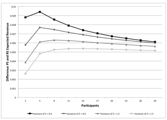
In Figures 4.1 to 4.3, each line represents the difference in expected revenue for a specific value of the variance oflog(S), which is denoted hereafter by σ2S. The darker the
line, the lower is the value ofσ2
S. This variation inσS2 can be interpreted as a difficulty in
estimating the costs of a pre-salt project. Thus, a higher variance of log(S) means that bidders cannot estimate costs accurately.
In these three graphs, we consider E[log(C)] = 1 and var(log(C)) = 2, which are denoted from this point forward by µC and σC2, respectively. Figure 4.1 presents
results with v = 1 (approximately 25% of the tracts are profitable), and Figures 4.2 and 4.3 exhibit results with v = 2 and v = 2.7 (approximately 50% of economic tracts), respectively.
Figure 4.1: Differences in Expected Revenues for Four Values ofσS2 and v = 1
The expected revenue difference seems to decrease as σ2
S increases, according to
Figure 4.2: Differences in Expected Revenues for Four Values ofσS2 and v = 2
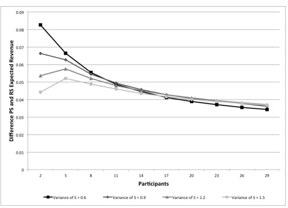
Figure 4.3: Differences in Expected Revenues for Four Values ofσS2 and v = 2.7
We also can represent cost uncertainty in various other ways. Now, we compute the difference in expected revenues for different levels in variance ofC. If we change var(C) and keep var(S) constant, there will be an improvement effect in estimating; i.e., it is as if the estimates of bidders became more accurate.
Thus, to isolate the effect of the variation ofvar(C), we consider proportional values of σ2
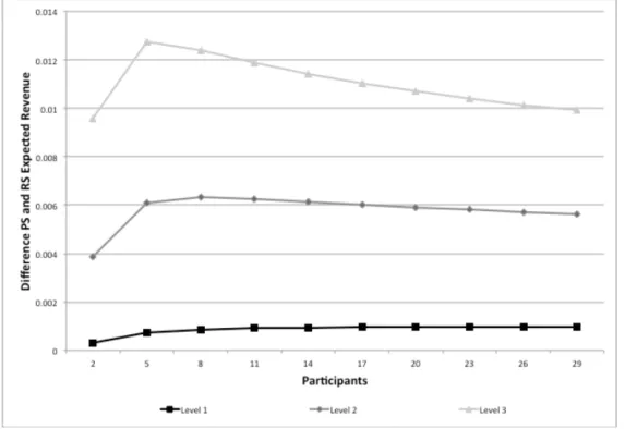
S. In the results of Figures 4.4 and 4.5, we assign σ2S = 0.3(σC2). However, it is not
possible to guarantee that the variance ofS will be perfectly proportional to the variance ofCbecauseSis an unbiased signal and follows a lognormal distribution; thus,var(S) will depend on the true value ofC. Moreover, becauseCalso follows a lognormal distribution, we must assign different values toµC and σ2C if we want to keep the same expectation of
C while var(C) changes.
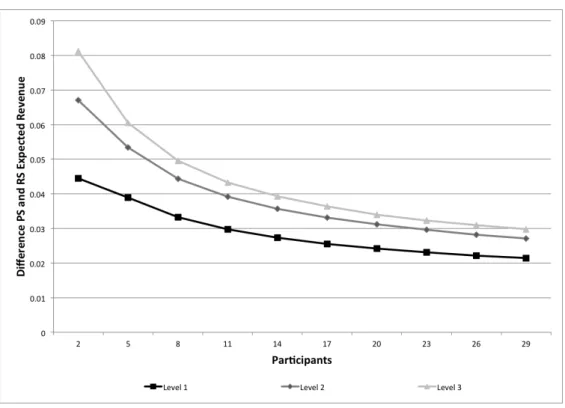
Table 1 exhibits the parameters used in Figures4.4 and 4.5:
Table 1: Levels of Variance of C for Figures 4.4 and 4.5
Level 1 Level 2 Level 3
µC 1 0.5 0
σC2 2 3 4
σS2 0.6 0.9 1.2
E[C] 7.4 7.4 7.4 var(C) 869 1690 2926
As we can see in Table 1, the values assigned to parameters µC and σ2C generate a
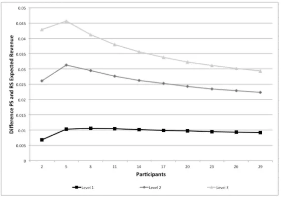
Figure 4.4: Differences in Expected Revenues for Three Levels of Variance ofC andv = 1
Figure 4.5: Differences in Expected Revenues for Three Levels of Variance ofC andv = 2
competitors in the auction.
Table 2: Levels of Variance of C for Figures 4.6 and 4.7
Level 1 Level 2 Level 3
µC 1.5 1 0.5
σC2 1 2 3
σS2 0.6 1.2 1.8
E[C] 7.4 7.4 7.4 var(C) 349 869 1690
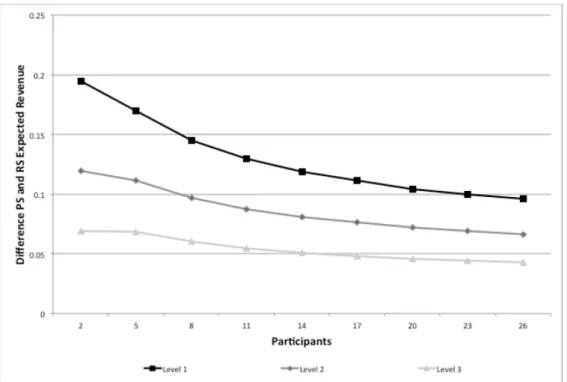
Table 2defines three levels of variance ofC, but with different values forµC andσC2
from those used in Table 1. For example, we set now σ2
S = 0.6(σC2). Figures 4.6 and 4.7
present results for these new parameter values, andv equals 1 and 2, respectively.
Figure 4.7: Differences in Expected Revenues for Three Levels of Variance ofC andv = 2
The order of curves presented by Figures4.6 and 4.7was the same as that observed in Figures 4.4 and 4.5. However, their shapes are flatter than before, particularly those associated with smaller variance. Thus, more competition is not so effective as to decrease the difference between the expected revenues in this case.
Figure 4.8: Differences in Expected Revenues for Three Levels of Variance of C and v at 25%
Figure 4.9: Differences in Expected Revenues for Three Levels of Variance of C and v at 60%
of profitable projects, the effect of variance of C yields completely different results than keeping v constant.
5
The New Regulatory Framework for the Brazilian Pre-Salt
Fields
In 1997, Brazil enacted the Petroleum Law (Law No. 9478), which regulated Con-stitutional Amendment No. 09/1995 and opened up exploration and production activities to local and foreign private investors. The Petroleum Law also regulated the concession agreement, which was the main regime for oil and gas exploration and production in Brazil until the more recent discoveries of the pre-salt oil fields.
In the concession regime, the winning consortium was determined by a formula that considers the amount of signing bonus (a one-time fee that is paid at the beginning of the contract), the minimum exploratory program and the percentage of local content used throughout the exploration and production period. Although the auctions were decided by these three criteria, as reported byMoura et al.(2012), in 95% of the blocks successfully auctioned, the winner offered the highest signing bonus.
The recent discoveries of the pre-salt oil fields led to the institution of a new regu-latory framework. Law No. 12351 of December 22, 2010 established a production sharing contract regime to be applied to licensing of the pre-salt reserves, in particular, and to other areas considered strategic by the government. In this new regime, government and oil companies (henceforth OCs) will share the profit generated by the production of oil and gas, allowing the government (the Union) to share a portion of the wealth yielded by the pre-salt fields.
Law No. 12351 defines some important concepts to understand this regime in details. Pursuant to Article 2 of Law No. 12351, cost oil is the “portion of oil production, by-products and other fluid hydrocarbons required only in event of commercial discovery, corresponding to costs and investments carried out by the contractor in the execution of the activities of exploration, evaluation, development, production and decommissioning of the facilities [...]”. Profit oil is defined as the “portion of the oil production, natural gas and other fluid hydrocarbons to be split between the Union and the contractor, according to criteria defined by contract, resulting from the difference between the total production volume and the portions related to the cost in oil, to the royalties due [...]”. The winning consortium is entitled to appropriate the cost in oil, plus its share of profit in oil, and both are enforceable only in case of commercial discovery.
for the auction to be used. According to the legal rules, the winner will be the bidder who offers the Union the highest share of profit oil, which thus means that the process embodies a profit-share bidding auction.
Article 4 of Law No. 12351 determines that Petrobras must be the sole operator of all blocks contracted under a profit-share regime. In assuming this role, Petrobras will be responsible for “running and executing, directly or indirectly, all exploration, evaluation, development, production and decommissioning of exploration and production installation activities” (Clause VI of Article 2 of Law No. 12351).
The operator is entitled to a minimum stake of 30% of the consortium. The tender protocol must indicate this mandatory share for the operator, given this minimum restric-tion. If Petrobras did not participate in the auction or was part of one of the defeated consortia, the winning bidder must form a new consortium with the Brazilian company. As part of this new consortium, Petrobras must adhere to tender protocol rules and win-ning bid terms. Moreover, proprietary rights and obligations will be proportional to the stakes of each member of the consortium.
In addition to a share of the profit oil, the winning bidder must pay the Union a signing bonus at the moment that the contract is executed and royalties at the rate of 15% of the value of production. The value of the signing bonus is fixed and predetermined in the tender protocol and is thus not part of the bid. The signing bonus and royalties cannot be reimbursed under any circumstances. In the event of commercial discovery, royalties will be subtracted from total production in the profit calculation, and the winning consortium will acquire the right to appropriate the production volume that corresponds to the royalties due. However, the same does not occur with respect to the value of the signing bonus, which is considered a non-recoverable cost.10
One important difference between the concession and profit-share models is the ownership of the oil extracted. In the concession regime, all oil extracted is owned by the concessionaire, and all the share payments (e.g., royalties) are converted using the market price for oil at that specific date. In the profit-share regime, however, the oil is owned by the Union, whether extracted or not. The parcel of oil extracted entitled to the winning bidder is the volume corresponding to the costs, royalties, and portion of profit oil that was bid. Therefore, the new rule reveals a government preference to keep the oil as opposed to pure monetary gains. Apparently, this decision is based on political rather than economic reasoning because the government could purchase the same amount of oil in the market after receiving the monetary payment corresponding to it.
In addition to Petrobras and other OCs, representatives of a public enterprise will be
10
Art. 2o