WIP - Workshop of Work in Progress

(1)

Desenvolvimento de um Sistema de Vis˜ao para

Inspeção Automática de Tecidos

Maur´ıcio Edgar Stivanello, Saulo Vargas Departamento de Metal-Mecˆanica IFSC - Instituto Federal de Santa Catarina

Florian´opolis, Brasil

Email:{mauricio.stivanello, saulo.vargas}@ifsc.edu.br

Juliano Emir Nunes Masson Departamento de Automac¸˜ao e Sistemas UFSC - Universidade Federal de Santa Catarina

Blumenau, Brasil

Email: [email protected]

Abstract—A number of defects can arise in the processes of spinning and weaving of textile industry. The identification of defective tissues in the early stages of the process reduces waste and discards. The objective of this work is to develop a system for automated inspection of fabrics. Statistical techniques based on intensity discontinuities on images of tissue are used to perform the detection of defective regions. The achieved results have shown the effectiveness of the employed approach for detecting different types of defects.

Keywords-automated inspection; computer vision; segmenta-tion; textile

Resumo—Uma série de defeitos podem surgir nos processos de fiação e tecelagem da ind ústria têxtil. A identificação de tecidos defeituosos nas etapas iniciais do processo reduz desperd´ıcios e devoluções. O objetivo do presente trabalho é desenvolver um sistema de inspeção automatizada de tecidos. Técnicas estat´ısticas de processamento baseadas na descontinuidade de intensidade das imagens dos tecidos são utilizadas para realizar a detecção de regiões defeituosas. Os resultados alcançados têm demonstrado a efetividade da abordagem proposta na identificação de diferentes tipos de defeito.

Keywords-inspeção automatizada; segmentação; tecido; visão computacional

I. INTRODUC¸ ˜AO

O cenário atual do mercado exige que a indústria têxtil aumente a eficiência, com linhas de produção mais ágeis, redução ao m´ınimo da criação de refugos e melhor qualidade de formação. Quando se considera o aumento do preço dos insumos, pequenos erros podem ser a fonte de grandes perdas na produção. Apesar de a qualidade ser essencial em qualquer tipo de economia, ela nunca foi tão importante quanto agora [1].

Na fabricação de tecidos, é essencial detectar os defeitos nos estágios iniciais do processo. Uma série de defeitos podem surgir nos processos de fiação e tecelagem, como os apresentados na Figura 1. Por exemplo, a detecção prévia de artefatos como passamento errado de malha, permite a classificação correta do tecido quanto a sua qualidade sem que um material defeituoso seja repassado aos processos de maior valor agregado, reduzindo assim os refugos e aumentando o rendimento. De modo geral, este tipo de inspeção reduz o vo-lume de refugos, aumenta o rendimento e diminui devoluções.

Figura 1. Exemplos de defeitos na produc¸˜ao de tecidos

A automação de etapas da produção tem se mostrado como uma excelente ferramenta para aumentar a agilidade da produção, sem redução de qualidade. Para o caso de identificação de defeitos em tecidos, por exemplo, podemos fazer uso desta ferramenta para minimizar a necessidade de inspeções manuais.

No presente trabalho é apresentado o desenvolvimento de um sistema de inspeção automatizada de tecidos empregando visão computacional. Na seção II são apresentadas estratégias normalmente utilizadas em inspeção automatizada. Na seção III é apresentada a abordagem proposta, utilizada no sistema implementado. Os resultados obtidos são descritos na seção IV. Finalmente, as conclusões são apresentadas na seção V.

(2)

desenrolando-os sobre uma mesa de inspeção a uma veloci-dade relativamente alta. Quando o inspetor humano percebe um defeito no tecido, ele para o motor que move o rolo, registra o defeito e sua localização, e inicia novamente o motor. Esta tarefa se mostra extremamente repetitiva e propensa a erros.

A visão computacional tem sido empregada com sucesso na análise ou inspeção automática em diferentes cenários. Os métodos utilizados para a inspeção de tecidos variam de acordo com as caracter´ısticas do tecido e são classificadas em três categorias, conforme a abordagem adotada para o reconhecimento do defeito: estat´ıstica, espectral e baseada em modelo [2].

A abordagem estat´ıstica pressupõem que as regiões do tecido livres de defeitos são de alguma forma estacionárias, o que torna poss´ıvel localizar na imagem inspecionada as regiões com comportamento estat´ıstico diferente. As abordagens dessa categoria se baseiam nos n´ıveis de intensidades das imagens dos tecidos e empregam técnicas como estimativa de dimensão fractal [3], estat´ısticas de n´ıvel de cinza, correlação cruzada, detecção de borda, operações morfológicas [4], matriz de co-ocorrência e transformação linear local [5].

Imagens de tecidos com textura uniforme, compostos por caracter´ısticas primitivas que possuem um padrão de repetição, são mais facilmente inspecionadas por abordagem espectral (que avalia o dom´ınio da frequência). transformadas de Fourier [6], filtro de Gabor [7], distribuição de Wigner [8] e transfor-mada Wavelet [9], são algumas das técnicas usadas para avaliar alterações espectrais desse tipo de imagem.

As abordagens baseadas em modelos são mais adequadas para imagens de tecidos texturizados aleatoriamente do que as abordagens estat´ısticas e espectrais. Nessa abordagem o tecido sem defeitos é modelado a partir de um processo estocástico, e o problema de detecção de defeitos passa a ser tratado como um problema de teste de hipóteses estat´ısticas do modelo. Modelo de Poisson [10] e campo aleatório de Markov Gauss [11] são exemplos de modelos empregados nessa abordagem.

III. METODOLOGIAPROPOSTA

No desenvolvimento do sistema apresentado, considerou-se como requisito principal a identificação de defeitos de forma automática na imagem do tecido inspecionado. Para atender a este requisito foi selecionado neste momento inicial de pesquisa a utilização de uma abordagem estat´ıstica. O flu-xograma das etapas de processamento utilizados é apresentado na Figura 2.

Na etapa de aquisição é realizada a captura de imagens digitais dos tecidos de interesse. Ainda nesta etapa, podem ser adicionados pré-processamentos, como a aplicação do filtro da mediana, por exemplo, para eliminar poss´ıveis ru´ıdos existentes.

Na etapa de segmentação é realizada a separação dos elementos de interesse da cena. Neste momento é necessário separar nas imagens a fase correspondente à textura original do tecido da fase correspondente aos defeitos presentes na amostra. Para isso, inicialmente é aplicada uma filtragem passa

Figura 2. Fluxo de processamento proposto para identificação automática de defeitos

banda com o objetivo de remover a textura repetitiva obtida em função do entrelaçamento dos fios do tecido. Em seguida é empregada a técnica de limiarização, combinada com o método de Otsu [12] para a determinação automática do valor de limiar para cada amostra inspecionada. Como sa´ıda da etapa de segmentação é obtida uma imagem binária onde os defeitos encontram-se destacados do fundo. Entretanto, em função de ru´ıdo ou outros artefatos presentes nas imagens adquiridas, pode ser obtido um grande número de pequenos componentes que não representam defeitos e que devem ser eliminados. Para isso, é empregada uma sequência de operações morfológicas de erosão e dilatação, de modo que apenas componentes com um tamanho pré-definido sejam mantidos.

Na etapa dedescrição cada um dos elementos restantes na imagem são detectados através de um algoritmo de rotulação de componentes conexos. Neste momento é gerada uma lista que contém a posição de cada elemento, além da área calcu-lada com base no número de pontos pertencentes ao mesmo. Por sua vez, na etapa de identificação os defeitos são encontrados de forma direta, avaliando-se a área de cada elemento e desconsiderando aqueles com valores fora de uma faixa aceitável. Finalmente, a partir das informações dos defeitos devidamente identificados e descritos é poss´ıvel levantar estat´ısticas ou mesmo enviar comandos a sistemas atuadores integrados à linha de produção.

IV. RESULTADOSEXPERIMENTAIS

O sistema descrito foi implementado em linguagem C++, utilizando a biblioteca de processamento de imagens OpenCV. Para validar o prot´otipo desenvolvido foi realizada uma bateria de testes utilizando a base de imagens de tecidos apresentada na Figura 3, onde as amostras apresentam diferentes tipos de defeitos [13].

(3)

Figura 3. Defeitos avaliados

defeito identificado, para as amostrasb ed. Os resultados ob-tidos com o algoritmo de identificação automática de defeitos que implementa o método descrito na seção III sobre a base de imagens de teste são apresentados na Tabela I.

Tabela I

RESULTADOS OBTIDOS NA INSPEC¸ ˜AO AUTOMATIZADA

Tipos de Tipos de Amostras com Amostras com defeitos Defeitos defeitos defeitos avaliados identificados identificados n˜ao identificados

12 10 a,b,c,d,e,f,g,h,j,l i,k

Os resultados obtidos são considerados promissores no que se refere à detecção automática, sendo que apenas dois dos defeitos avaliados não foram corretamente identificados. O algoritmo implementado é simples de ser utilizado. O valor de limiar utilizado na segmentação é obtido satisfatoriamente pelo método de OTSU, sendo que apenas a definição dos parâmetros do filtro passa banda, que é dependente da textura do tecido, se faz necessária.

Na Tabela II são apresentados os tempos médios necessários ao processamento das principais etapas envolvidas. Para o pro-cessamento de todo o ciclo de inspeção foi obtido um tempo

Figura 4. Ilustração do Processo de Identificação

médio de 10,46ms em um computador com processador INTEL Core i7-4500U de 1.80 GHz e 8GB de memória RAM, sobre amostras de 690 X 682 pixeis. É importante observar que os algoritmos podem ainda ser otimizados empregando recursos espec´ıficos de hardware.

Tabela II

TEMPOS MEDIOS DE PROCESSAMENTO´

Etapa Tempo (ms)

Aquisição e pré-processamento 8,24

Segmentac¸˜ao 0,10

Descrição, identificação e extração de dados 2,09

Fluxo geral 10,43

´

E importante avaliar os tempos de processamento obtidos frente ao dom´ınio do problema. O sistema proposto será integrado a uma máquina revisora já em uso na indústria, conforme ilustrado na Figura 5, de modo a automatizar a etapa de inspeção de defeitos.

(4)

Figura 5. Ilustração da implantação em máquina revisora

câmera no sentido transversal do tecido inspecionado, de modo a cobrir rolos de tecido com larguras que excedam o campo de visão da câmera.

V. CONCLUSOES E˜ PERSPECTIVAS

No presente trabalho foi apresentado o desenvolvimento de um sistema de identificação automática de defeitos em tecidos por meio de visão computacional. O sistema corrente, que ainda se encontra em um estágio inicial de desenvolvimento, apresentou resultados satisfatórios na identificação de diferen-tes tipos de defeitos. Desta forma, sua utilização de forma integrada a linhas de produção para controle de qualidade mostra-se promissora.

Como perspectivas futuras, pretende-se aumentar a robustez do sistema e ampliar a gama de defeitos detectados através da combinação das técnicas estat´ıstica, espectral e baseada em modelo, conforme sugerido por Kumar [2]. A validação do sistema nas versões futuras será realizada sobre uma base de imagens maior do que a utilizada neste trabalho, empregando um conjunto de imagens que está sendo criado a partir de amostras de tecidos obtidos junto à indústria têxtil. Quando o sistema apresentar robustez e eficiência adequadas, pretende-se integrar o mesmo uma máquina revisora de tecidos, de modo a avaliar a sua efetividade em condições reais de uso.

AGRADECIMENTOS

Os autores gostariam de agradecer ao CNPq pelo suporte financeiro provido para a realizac¸˜ao do projeto na qual este estudo foi realizado.

REFERENCIASˆ

[1] L. C. Rodrigues, C. E. N. Bizzotto, and D. Souza, “Estratégias compe-titivas no setor têxtil na região de blumenau,” inAnais do XIX Simpósio de Gest ao da Inova’cão Tecnológica, 1996.

[2] A. Kumar, “Computer-vision-based fabric defect detection: A survey,” IEEE Transactions on Industrial Electronics, vol. 55, pp. 348–363, 2008. [3] A. Conci and C. B. Proenc¸a, “A fractal image analysis systems for fabric inspection based on a box-counting method,”Comput. Netw. ISDN Syst., 1998.

[4] Y. F. Zhang and R. R. Bresee, “Fabric defect detection and classification using image analysis,” Textile Research Journal, vol. 65, pp. 1–9, January 1995.

[5] C. Neubauer, “Segmentation of defects in textile fabric,” inPattern Re-cognition, 1992. Vol.I. Conference A: Computer Vision and Applications, Proceedings., 11th IAPR International Conference on, 1992.

[6] R. N. Bracewell,The Fourier transform and its applications, 3, Ed. McGraw-Hill, 2000.

[7] A. Bodnarova, M. Bennamoun, and S. J. Latham, “Textile flaw detection using optimal gabor filters,” inPattern Recognition, 2000. Proceedings. 15th International Conference on, 2000.

[8] K. Song, M. Petrou, and J. Kittler, “Texture crack detection,”Machine Vision and Applications, 1995.

[9] H. Sari-Sarraf and J. S. Goddard, “Vision system for on-loom fabric inspection,”Industry Applications, IEEE Transactions on, 1999. [10] D. P. Brzakovic, P. R. Bakic, and A. Liakopoulos, “An approach to

quality control of texture web materials,” inSPIE 2597, 1995. [11] X. Z. Yang, G. K. H. Pang, and N. H. C. Yung, “Discriminative fabric

defect detection using adaptive wavelets,”Optical Engineering, 2002. [12] N. Otsu, “A threshold selection method from gray-level histograms,”

IEEE Transactions on Systems, Man and Cybernetics, vol. 9, pp. 62– 66, 1979.

(5)

Gesture Recognition using shape characteristics

Igor L. O. Bastos Math Institute Federal University of Bahia

Salvador, Brazil [email protected]

Michele F. Angelo, Angelo C. Loula Dept. of Technology, Dept. of Exact Sciences

State University of Feira de Santana Feira de Santana, Brazil

[email protected], [email protected]

Abstract —The present work brings up a system for recognizing gestures using two (2) shape descriptors, the histogram of oriented gradients (HoG) and Zernike invariant moments. These are used together to feed a two stage classifier composed of Artificial Neural Networks that perform the gesture classification. To train and test the classifier, 2208 images were used representing 12 signs from the Brazilian sign language (Libras). High accuracy rates were obtained, reaching in average 94% of accuracy for all 12 signs.

Index Terms — Histogram of oriented gradients, Zernike moments, Artificial Neural Networks.

I.INTRODUCTION

Gesture recognition pertains to recognizing meaningful expressions of motion by a human, involving hands, arms, face, head, and/or body [1]. Many techniques and strategies have been used on last years [2] ranging from works where digital image processing is exclusively used to systems that use computer vision and classification based on feature extraction.

Among the many fields where gesture recognition is applied, the field of signal languages is an important one. One of these languages is the Brazilian Sign Language (Libras), which is considered, since 2002, as an official Brazilian language [3].

In this context fits the present work. It describes the development of an approach for recognition of 12 signs from Libras. This approach takes as input images containing the hand signals and presents, at the end of the recognition process, the recognized sign as a response. Note that the signs from Libras present parameters, which include body language, movement and orientation [3]. However, for this work, only the hand configuration is used and signs are recognized statically.

II.RELATED WORK

Works applying computer vision techniques for gesture recognition have greatly increased in the last years [4]. Some of them are closely related to the present work.

The project proposed by Carneiro, Cortez and Costa [5] presents an approach for classifying signs from Libras using neural networks. However, the features used by Carneiro for classifying signs were Hu Invariant Moments. This project recognized 26 signals from Libras and showed accuracy rates ranging from 78% to 97%.

The project proposed by Rodriguez, Chavez and Menotti [6] used the classifier Support Vector Machine (SVM) to perform the classification. In this study, 24 Libras signs were recognized using the descriptors Hu invariant moments and Zernike invariant moments. These descriptors were used separately and the results obtained with them were compared. The Zernike descriptor showed better results, reaching, for some signs, 96% of accuracy rate.

Besides the existence of works related to Libras, others were found using similar approaches for recognizing signs from other languages as the one proposed by Bowden [7], which operates by recognizing signs of British Sign Language (BSL). It also uses a two stage classification process where shape features are extracted from hand images. This work also operates with non-static signs and to recognize them, motion features are also extracted and Hidden Markov Models (HMM) are used to perform the classification of these signs.

III.THEORETICAL FOUNDATION

In order to recognize the signs from the input images, shape-based features are used to extract information that allows the system to recognize the sign present from the input image. These feature descriptors are the Histogram of Oriented Gradients (HoG) and Zernike Invariant Moments.

A.Histogram of Oriented Gradients

Histograms of Oriented Gradients (HoG) are gradient based feature descriptors that are commonly used for object detection and recognition [8].

HoG’s functionality is based on the principle that the shape of an object can be described by the distribution of intensity gradients and edge directions. To achieve a more precise representation of the shape of an object, the input (image) is divided in small regions called cells. For each cell the descriptor is computed and the final result consists on the output for all cells.

In addition, some parameters of HoG have to be adjusted. The size of cells and blocks (group of cells to perform gradient strength normalization), number of bins and the use or not of the orientation of gradients are some of these parameters.

B.Zernike Invariant Moments

(6)

information between the moments [9]. Because of these characteristics, Zernike moments have been used in pattern recognition applications [6, 10], like the present project.

One of the most important characteristic of the Zernike moments is the independence of their magnitude to the rotation. Hence, they can be used to describe shape characteristic of objects on images [9]. For the present project, where the input images can present variation in terms of rotation of the hands (Libras signs), these moments proved to be appropriated.

The Zernike moments are defined by two parameters: order and repetition. They differ on a rotated image from those of the original unrotated image in phase shifts, but no in magnitudes [11]. So, these magnitudes can be used as a rotation invariant feature.

IV.METHODOLOGY

The methodology used in this study started with the building of the training image dataset, followed by feature selection and data classification in two stages.

A.Composing the training dataset

The present work intends to classify gestures from the Brazilian Sign Language (Libras). As this work represents an intermediate stage in the development of a bigger project, which aims at recognizing about 50 distinct signs from Libras, it was decided that it would recognize 12 signs that represent letters of the Libras alphabet [3]. The selected gestures are the signs A, B, C, D, E, G, I, L, O, U, W and Y. They were selected because the HoG descriptor and the Zernike moments are shape-based features and these gestures have a very different shape one from another signs.

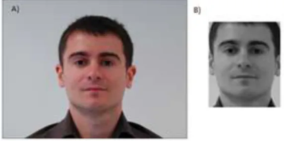
A database containing 1104 grayscale images was built for these 12 different Libras signs. These images have resolution of 50 by 50 pixels and contain the hand positions that represent the selected signs from Libras. All images were taken using only one person as model and for a better image acquisition, the light conditions were controlled. On Figure 1, some of these images can be seem.

Fig. 1. Images representing Libras signs. a) letter A. b) letter B. c) letter C. d) letter D.

On the other hand, an auxiliary dataset was composed with another 1104 images. They are binary masks obtained with a skin detection approach [12] applied on the original images (RGB images before converting them to grayscale) and represent the skin zones of the 1104 images obtained before (Figure 2).

Fig. 2. Binary masks representing the signs. a) letter A. b) letter B. c) letter C. d) letter D.

To grant to the classifier the ability to recognize gestures that have variations on the positions, the dataset was built with images presenting variations in rotation, and variations resulting from the acquisition process and skin recognition (Figure 3).

Fig. 3. Images of dataset showing rotational variance and acquisition variance

B.Extracting features from the images

To extract relevant information from the images, the HoG descriptor and the Zernike moments were applied in order to generate a feature vector. The HoG descriptor, to be associated to the edges (gradients) of the image, was applied directly on the grayscale images. On the other hand, to apply the Zernike moments, that is associated to the shape of objects on images, it was necessary to use the binary masks over the grayscale images, applying the Zernike descriptor on the resulting images.

C.Selecting features

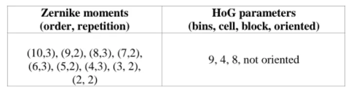
As it was mentioned before, the histogram of oriented gradients (HoG) and the Zernike invariant moments were used to compose a feature vector used to feed the classifier because of their shape-based character. To select the parameters of HoG, as number of bins and size of blocks and cells; and the order and repetition of Zernike moments that would be used, tests were performed and the accuracy of the classifier was measured, considering the variation of these parameters. The selected parameters of both descriptors were those for which the classifier had the highest accuracy rates.

Table 1 shows the selected parameters for both descriptors.

TABLE I. SELECTED FEATURES

Zernike moments (order, repetition)

HoG parameters (bins, cell, block, oriented)

(10,3), (9,2), (8,3), (7,2), (6,3), (5,2), (4,3), (3, 2),

(2, 2)

9, 4, 8, not oriented

D.Assembling the groups

As mentioned before, 12 signs from the Libras alphabet were chosen to be recognized. Those gestures were grouped into 3 small groups (each with 4 gestures).

(7)

different patterns, it would probably be necessary to have a large number of neurons in its hidden layers. This could cause problems such as an increase in computational cost / time for training and classification, as well as other possible problems, such as excessive adaptation to the trained patterns (overfitting).

So, it was decided that the classification would be performed in 2 stages: 1) Recognition of the group which the input image belongs. 2) Recognition of the sign of the input image.

Deciding the signs that would compose each group was the first task to be done. As the HoG and Zernike moments are shape descriptors, we chose to put similar signs (those that present conformable shape) in the same group. The visual inspection was the only criteria to do this grouping. Thus, we have reached: Group 1: “A”, “B”, “E” and “G”; Group 2: “C”, “D”, “O” and “W”; Group 3: “I”, “L”, “U” and “Y”.

Images from each group can be seen on Figure 4.

Fig. 4. Signs of each group.

E.Architecture of the classifier

The architecture of the neural network classifier used is shown on Figure 5.

Fig. 5. Architecture of the used classifier.

The recognition of the input gesture is performed in two stages. The first one corresponds to a group classification, which is conducted by a neural network trained with images of

all 12 gestures. The goal of this network is to recognize the group that the input belongs and lead the classification to a next neural network. The output of the general classification determines which subsequent network should be activated. As shown in Figure 5, these subsequent networks are trained to classify individual gestures of a single group and the output of them is the sign to which the input corresponds.

Tests were also performed in order to decide the number of hidden neurons. For the first network (general classification), 45 hidden neurons were used, once it provided a better performance. For the ones responsible for groups 1 and 3, 25 hidden neurons were used. The one responsible for group 2, presented better results using 18 hidden neurons. The results showed on next section were done using these configurations.

V.RESULTS AND DISCUSSION

In order to validate the proposed system, a testing dataset was generated. It was modeled in the same way as the training dataset, which had grayscale images and binary masks. The test images, as well as training, have a resolution of 50 by 50 pixels and this dataset was composed by 2400 images.

The first part to be tested on the present system was the first network (group classification). This network was tested with images from all 12 trained Libras signs and the response was checked to see if it matches the correct group. The results obtained with this classification are shown on Figure 6, where the average accuracy rate for each group can be seen.

Fig. 6. Average group recognition accuracy rate for each group.

(8)

Fig. 7. Average group recognition rates

As shown on Figure 7, the recognition rates for all signs were above 85% of accuracy. It is also noticeable that, for signs “A” and “G”, the rates were lower than for the others. That promoted the performance drop for this first group compared to the others.

Lastly, the accuracy of the two stage classification of each gesture was determined and is shown on Figure 8.

Fig. 8. Final recognition for each gesture

Figures 6, 7 and 8 evidenced that the system developed obtained high accuracy rates. For all gestures, the recognition rate was above 84%. Final (two stage) gesture recognition rates for each sign were very similar to group recognition ones. This evidences that the individual gesture recognition performed well for gestures corrected classified at the first stage.

Gestures “A” and “G” showed the lowest recognition rates. Both cases can be associated to the similarity of these gestures with gestures of other groups, what was pointed by the group classifier performance shown on Figure 7. That evidences that, if only one network was used, the system could have problems to distinguish all the 12 gestures.

VI.CONCLUSION

Despite the not so high rates for the recognition of the "A" and "G", the system presented good results, with an average recognition rate of about 94%. Some changes on the group organization (change the gestures of each group) could result in better results.

As future work, we hope to extend the system to recognize more signs from Libras (about 50), besides seeking a better strategy to distribute the gestures on groups. It would propitiate a gain in terms of accuracy for signs that the results were not as high, as "A" and "G".

REFERENCES

[1] S. Mitra and T. Acharya, “Gesture Recognition: A Survey,” IEEE Transactions on Systems, Man and Cybernetics – Part C: Applications and Reviews, vol. 37, n. 3, May 2007.

[2] V. Pavlovic, R. Sharma and T. Huang, “Visual Interpretation of Hand Gestures for Human-Computer Interaction: A Review,” IEEE Transactions on Pattern Analysis and Machine Intelligence, vol. 7, n. 7, July 1997.

[3] T. Felipe, A Libras em Contexto, 8th ed., Walprint Gráfica e Editora, 2007.

[4] R. Khan and N. Ibraheem, “Survey on Gesture Recognition for Hand Image Postures,” Computer and Information Science Journal, vol. 5, n. 3, May 2012.

[5] A. Carneiro, P. Cortez and R. Costa, “Reconhecimento de gestos da Libras com classificadores neurais a partir dos momentos invariantes de Hu,” Interaction South America, 2010.

[6] K. Rodríguez, G. Chávez and D. Menotti, “Hu and Zernike Moments for Sign Language Recognition,” International Conference on Image Processing, Computer Vision and Image Recognition, 2012.

[7] R. Bowden, D. Windridge, T. Kadir, A. Zisserman and M. Brady, “A Linguistic Feature Vector for the Visual Interpretation of Sign Language,” European Conference of Computer Vision, 2004.

[8] N. Dalal and B. Triggs, “Histograms of Oriented Gradients for Human Detection,” IEEE Computer Society Conference on Computer Vision and Pattern Recognition, vol. 1, pp. 886-893, 2005.

[9] S. Hwang and W. Kim, “A novel approach to the fast computation of Zernike moments,” Journal of Pattern Recognition, vol. 39, pp. 2065-2076, March 2006.

[10] A. Khotanzad and Y. Hong, “Invariant Image Recognition by Zernike Moments,” IEEE Transactions on Pattern Analysis and Machine Intelligence, vol. 12, n. 5, May 1990.

[11] H. Hse and A. Newton, “Sketched Symbol Recognition using Zernike Moments,” Proceedings of the 17th_{International} Conference on Pattern Recognition, vol. 1, 2004.

(9)

Segmentação e Classificação de Embarcações em

Eclusas

Fagner Pimentel∗, Michele F´ulvia Angelo†, Diego Gervasio Fr´ıas‡ ∗ _{Universidade Federal da Bahia - UFBA}

† _{Universidade Estadual de Feira de Santana - UEFS}

Email: [email protected] ‡_{Unversidade do Estado da Bahia - UNEB}

Abstract––This paper aims to identify and classify ships in river environments using and comparing techniques for segmentation like Background Subtraction and classifiers like Support Vector Machine. This study is expected to define a set of techniques that best fit the segmentation and classification of ships in river environments in order to optimize the flow of ships at locks located on the Tietˆe river as future application.

Keywords––Segmentation; Classification; Ship; Fluvial Environment;

Resumo––Este trabalho tem como objetivo identificar e classificar embarcações em ambientes fluviais usando e comparando técnicas de segmentação como subtração de background e classificadores como Support Vector Machine. Este estudo deverá definir um conjunto de técnicas que melhor se adequam a segmentação e classificação de embarcações em ambientes fluviais, a fim de otimizar o fluxo de embarcações em eclusas localizadas no rio Tietê como aplicação futura.

Palavras-chave––Segmentação; Classificação; Embarcação; Ambiente fluvial;

I. INTRODUC¸ ˜AO

Uma eclusa é uma obra de engenharia hidráulica que permite uma embarcação vencer o desn´ıvel de uma barragem, quedas de água ou corredeiras no leito do curso d’água [1], [2]. O processo de eclusagem é iniciada quando uma embarcação chega ao ponto de parada obrigatória (PPO) da jusante (ponto mais baixo do rio) ou montante (ponto mais alto do rio).

A hidrovia Tietê-Paraná no estado de São Paulo, conta com seis eclusas: uma em Barra Bonita, a primeira usina na cascata do rio Tietê, com eclusagem voltada principalmente para o turismo; uma em Bariri com eclusagem voltada para o transporte de cana de açúcar; uma em Ibitinga voltada para o turismo e para carga; uma em Promissão; e por fim, duas em Nova Avanhandava por possuir um canal de eclusagem muito longo. Nesta última existe apenas um operador para as duas eclusas com controle centralizado. As usinas, eclusas e barragens de Barra Bonita, Bariri, Ibitinga, Promissão e Nova Avanhandava são mantidas e operadas pela concessionária AES/Tietê [3].

As passagens nas eclusas são realizadas 24 horas por dia, ininterruptamente, salvo em casos de emergência, relacionados à segurança ou por solicitação da operadora das eclusas. O tempo para realizar a eclusagem nas eclusas do rio Tietê

varia entre 20 e 45 minutos, dependendo fundamentalmente das vazões de enchimento e drenagem pelas comportas e do n´ıvel do reservatório. O direito de passagem na eclusa para as embarcações que estejam aguardando, é concedido pelo operador da eclusa considerando a seguinte ordem de prioridade: (1) Embarcações da Marinha do Brasil, Órgãos de fiscalização federal, estadual e municipal em embarcações ofi-ciais; (2) Embarcação comercial de passageiros (turismo); (3) Embarcação destinada à execução de trabalhos de manutenção na hidrovia; (4) Embarcação transportando mercadorias pe-rec´ıveis ou suscept´ıveis de perdas na qualidade final do produto; (5) Embarcação de lazer (esporte e recreio), sendo as embarcações de turismo e mercadoria as que trafegam com mais frequência.

Na ausência de embarcações que preencham os requisitos acima, é considerada como prioridade a ordem de chegada da embarcação nos PPO’s (jusante e montante) da eclusa [1]. Após finalizar uma eclusagem o operador envia os dados (tipo de embarcação e horário previsto de chegada) no sentido montante ou jusante, para que o operador da próxima eclusa esteja preparado.

Conforme descrito , a identificação das embarcações é feita pelo operador da eclusa, e o controle de prioridade para entrar na eclusa se dá de forma manual, sem qualquer tipo de otimização, possibilitando maior ocorrência de erros no con-trole e gastos desnecessários, como por exemplo, no tempo de espera das embarcações e vertimento da água utilizada. Com base neste contexto, a proposta deste trabalho é desenvolver um sistema de segmentação e classificação de embarcações em ambientes fluviais a partir de imagens extra´ıdas do sistema de vigilância da concessionária AES/Tietê que utilizam câmeras do tipo Pan-Tilt-Zoom, capazes de realizar movimentos na vertical (Pan), horizontal (Tilt) e de aproximação (Zoom).

(10)

II. TRABALHOS RELACIONADOS

Em [4], no contexto de detecção de embarcações, o classi-ficador SVM (do inglês, Support Vector Machine) é utilizado para reconhecer primeiramente regiões que representam água, para que em seguida seja feita a busca por embarcações nesta região. A abordagem é baseada nas seguintes observações no cenário de vigilância: as embarcações só podem viajar dentro da região de água, e o movimento das embarcações é mais relevante do que o movimento das regiões de água. Partindo do pressuposto que as embarcações apenas trafegam dentro da região de água, a detecção de embarcações pode ser facilitada se a região de água for extra´ıda e fornecida como informação contextual.

Em [5] é aplicada a subtração de background juntamente com um duplo threshold (hysteresis) para a segmentação de embarcações. Como acontece normalmente em imagens com background dinâmico, não somente o movimento das embarcações como também da água e das árvores são captados pela subtração de background. A ideia do threshold com hysteresis é explorar a coerência espacial do objeto na imagem resultante da subtração. Nesta abordagem, primeiramente, é passado um threshold alto, determinando um subconjunto de pixels do objeto, em seguida um threshold baixo contendo um subconjunto maior de pixels. O resultado final é dado pelos pixels de baixo threshold que se interligam recursivamente aos pixels de alto threshold.

Em [6] é utilizada a subtração de background para o rastreamento de embarcações em ambientes mar´ıtimos, onde a maior parte do background é formado pelo oceano. A principal dificuldade neste trabalho está no fato do oceano ser dinâmico e os objetos terem que ser extra´ıdos em um ambiente altamente imprevis´ıvel. Neste trabalho foi desenvolvido um algoritmo próprio de subtração de background além de utilizar a t´ıtulo de comparação, algoritmos do tipo Mistura de Gaussiana [7] e Sigma-Delta[8].

Em [9] foi utilizada uma RNA (Rede Neural Artificial) para a classificação de embarcações com 12 neurônios de entrada, 20 neurônios na camada escondida e 5 na camada de sa´ıda. Foram utilizadas 240 imagens para o treinamento, variando os ângulos de visão das embarcações. Ao final do treinamento foi obtida uma taxa de acerto de 90.1%. Em seguida foram realizados testes com 41.400 imagens, obtendo uma taxa de acerto de 87.3%.

Em [10] foi utilizado um classificador SVM para classificar embarcações a partir de câmeras Pam-Tilt-Zoom e HOG (do inglês Histogram of Oriented Gradients) como extrator de caracter´ısticas. Para o treinamento do classificador foram utilizadas 280 imagens positivas e exemplos do background extra´ıdo como imagens negativas, obtendo uma taxa de acerto de 85%.

III. METODOLOGIA

O projeto tem como objetivo segmentar e classificar embarcações em rio através de imagens de câmeras pan-tilt-zoom (Figura 1), e o seu desenvolvimento será dividido nas seguintes etapas:

Figura 1. Visão Geral do projeto: A partir do (a) campo de visão da câmera a embarcação é colocada em foco usando pan-tilt-zoom, gerando as imagens que servem de (b) input para o sistema, em seguida é realizada a (c) Segmentação da embarcação e classificação da segmentação em embarcação de turismo ou carga.

A. Criac¸˜ao do Dataset

Serão criados datasets com marcações em binary mask para a fase de avaliação dos algoritmos de subtração de background e para o treinamento e testes dos classificadores. Estes datasets serão criados com imagens positivas (exemplos de embarcações) e negativas (background) das esclusas ao longo do rio Tietê.

Para a criação destes datasets serão selecionados v´ıdeos for-necidos pela concessionária AES/Tietê que possuam exemplos das embarcações que trafegam pelas eclusas em diferentes mo-mentos e com diferentes luminosidades, ângulos e distâncias. Os datasets de binarymask serão criados com a ajuda de uma ferramenta de anotação semi-automática desenvolvida para este propósito. Com esta ferramenta será poss´ıvel criar o dataset a partir de um v´ıdeo selecionado.

B. Segmentac¸˜ao

Nesta etapa será realizado um pré-processamento das ima-gens visando identificar as regiões de água, servindo de informação de contexto para facilitar a segmentação da embarcação.

Em seguida será realizado um estudo de performance de 27 algoritmos de subtração de backgroung implementados na biblioteca bgslibrary [11] com o objetivo de escolher o algoritmo que apresente bons resultados para as imagens que serão utilizadas neste projeto.

O algoritmo de bakground que apresentar o melhor resul-tado ser´a adapresul-tado para utilizar a t´ecnica de threshold com hysteresis observado em [5].

C. Extrac¸˜ao de Caracter´ısticas

Segmentada a embarcação, o próximo passo é extrair as caracter´ısticas que a descrevam. A principal caracter´ıstica que será utilizada para a classificação de embarcação será a forma. Segundo Luoet al. 2006 [5], a forma é a caracter´ıstica mais importante para a detecção de embarcações.

Um método que será utilizado para a extração de carac-ter´ısticas de embarcações será o histograma de gradientes orientados (HOG) [10]. A ideia deste método é que a forma dos objetos pode ser caracterizada pela direção e intensidade dos gradientes em uma imagem.

(11)

D. Classificac¸˜ao

Nesta etapa será utilizado o classificador SVM (Suppport Vector Machine) como foi usado em [12], [10], previamente treinado. A priori serão classificadas as embarcações volta-das para o turismo e para o transporte de carga por serem as que trafegam com mais frequência nas eclusas. Após a implementação das técnicas e treinamento dos classificadores, serão realizados os testes com as imagens e v´ıdeos separados para esta finalidade.

IV. RESULTADOSPRELIMINARES

Até o presente momento a etapa A (Criação do Dataset) foi finalizada parcialmente e a etapa B (Segmentação) foi finalizada. As etapas C (Extração de Caracter´ısticas) e D (Classificação) estão em desenvolvimento. A seguir os resul-tados preliminares serão apresenresul-tados.

A. Criac¸˜ao do Dataset

Foi construido um dataset a partir de imagens capturadas da eclusa de Nova Avanhandava. O dataset é composto de 5 v´ıdeos de embarcações se aproximando da eclusa com uma média de 1280 frames por v´ıdeo. Cada v´ıdeo contem uma embarcação em um ambiente com carros, árvores, nuvens e água em movimento e variação de luminosidade ao longo do dia. Nestes v´ıdeos foram realizadas as anotações de ground-truth em binarymask com o aux´ılio de uma ferramenta de anotação semi-automática desenvolvida para facilitar e acelerar este processo.

Esta ferramenta de marcação, primeiramente, cria os frames com uma pré-anotação feita automaticamente utilizando um simples algoritmo de subtração de background. Em seguida, cada frame é editado manualmente fazendo as correções necessárias sobre a pré-anotação. Para facilitar e acelerar o processo, a ferramenta conta com uma interface que auxilia a mudança rápida entre os frames, auxilia a verificação da anotação sobrepondo a imagem original e possui regulagem do marcador, além da utilização de uma mesa digitalizdora.

Este dataset foi utilizado para a avaliação dos algoritmos de background e para a realização do treinamento e validação do classificador de água.

B. Segmentac¸˜ao

Esta etapa foi dividida em duas sub-etapas, uma responsável pela identificação da água do rio (pré-processamento) e outra para a avaliação dos algoritmos de background e adaptação do melhor algoritmo encontrado.

1) Identificação da água do rio: Nesta etapa, primeira-mente, foram recortados segmentos de imagens com exemplos positivos e negativos de água a partir de cada v´ıdeo do dataset das eclusas. Com isso foi poss´ıvel criar cinco conjuntos de treinamento e teste, onde cada conjunto de treinamento utiliza imagens de quatro v´ıdeos e cada conjunto de teste utiliza imagens do v´ıdeo restante, tornando os conjuntos mutualmente exclusivos.

Para a extração das caracter´ısticas da água do rio, foi realizada em cada imagem dos conjuntos de treinamento e

Tabela I

RESULTADO DOS TESTES DE CLASSIFICAC¸ ˜AO DEAGUA.´

linear polynomial base radial sigmoid

Data 1 98.0% 98.0% 97.6% 66.6%

Data 2 99.6% 99.6% 64.6% 66.6%

Data 3 100.0% 100.0% 100.0% 66.6%

Data 4 100.0% 98.3% 98.3% 66.6%

Data 5 94.6% 93.0% 92.0% 66.6%

teste a transformação do espaço de cor RGB para LAB e utilizadas as caracter´ısticas A e B, as quais representam as cores, e ignorada a caracter´ıstica de luminosidade L.

O classificador utilizado foi o SVM e os resultados obtidos, variando-se o kernel em linear, polynomial, de base radial e sigmoid são mostrados na Tabela I. Através desta tabela pode-se verificar que o SVM com kernel linear obteve os melhores resultados, com uma média de acerto de 98.4% e por isso escolhido neste trabalho.

Por fim, foi realizada a segmentação de regiões similares no frame inicial de cada v´ıdeo, utilizando um algoritmo de segmentação de regiões proposto em [13]. Em seguida cada região é classificada como água ou não água utilizando-se o classificador SVM com kernel linear, treinado previamente a partir de caracter´ısticas de cor do espaço de cor LAB.

O pré-processamento para a identificação de água é reali-zado apenas no primeiro frame do v´ıdeo, partindo da hipótese que a região de água não será alterada nos frames seguintes.

2) Avaliação dos algoritmos de subtração de background: Dado que para a realização da subtração de background é necessária uma câmera estática, esta fase é realizada apenas nos momentos em que a câmera está parada.

Tendo em vista a eficiência do threshold com hysteresis observado em [5], a avaliação dos algoritmos de subtração de backgrund foi realizada visando a aplicação desta técnica no algoritmo selecionado. O melhor algor´ıtmo foi encontrado através da média harmônica (HM) da taxa de verdadeiros positivos (TPR) e a taxa de verdadeiros negativos (TNR). O TPR é definideo por TP / (TP+FN), enquanto o TNR é definido por TN / (FP + TN) e o HM é 2*TPR*TNR / (TPR + TNR), onde TP é número de verdadeiros positivos, TN é o número de verdadeiros negativos, FN é o número de falsos negativos, e FP é o número de falsos positivos.

A partir dos dados extra´ıdos das métricas de avaliação dos algoritmos, foram feitas comparações a fim de determinar qual algor´ıtmo melhor se aplica ao projeto. Para cada um dos v´ıdeos presentes no dataset foram feitas 27 avaliações referentes a cada algoritmo da biblioteca bgslibrary [11], utilizando a média harmônica da taxa de verdadeiros positivos e a taxa de verdadeiros negativos apresentada anteriormente. Dada a grande quantidade de algoritmos, os parâmetros dos mesmos foram mantidos como padrão da biblioteca bgslibrary.

(12)

Tabela II

M ´EDIA HARMONICAˆ (HM)DA TAXA DE VERDADEIROS POSITIVOS E A TAXA DE VERDADEIROS NEGATIVOS PARA CADA ALGORITMO.

algoritmo HM

AdaptiveBackgroundLearning 0.7124

DPAdaptiveMedianBGS 0.4712

DPEigenbackgroundBGS 0.9528

DPGrimsonGMMBGS 0.7078

DPMeanBGS 0.2112

DPPratiMediodBGS 0.5903

DPTextureBGS 0.8430

DPWrenGABGS 0.6530

DPZivkovicAGMMBGS 0.7853

FrameDifferenceBGS 0.3663

FuzzyChoquetIntegral 0.4131

FuzzySugenoIntegral 0.3797

GMG 0.8025

KDE 0.8120

LbpMrf 0.8253

MixtureOfGaussianV1BGS 0.2342 MixtureOfGaussianV2BGS 0.3457

MultiLayerBGS 0.3514

PixelBasedAdaptiveSegmenter 0.2889 StaticFrameDifferenceBGS 0.9167

T2FGMM UM 0.1812

T2FGMM UV 0.6851

T2FMRF UM 0.1694

T2FMRF UV 0.4589

VuMeter 0.2902

WeightedMovingMeanBGS 0.2595 WeightedMovingVarianceBGS 0.2890

embarcac¸˜oes em ambientes fluviais neste trabalho.

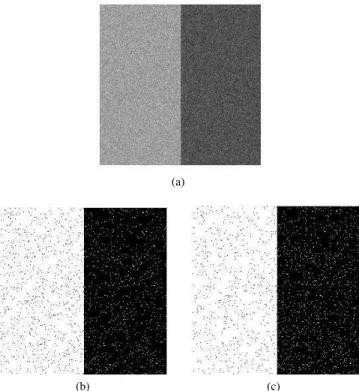
Sobre o algoritmo DPEigenbackgroundBGS foi aplicado o hysteresis. Na Figura 2 é poss´ıvel observar os resultados para o reconhecimento de água (Figura 2b), o threshold alto (Figura 2c), o threshold baixo (Figura 2d), o resultado da aplicação do hysteresis (Figura 2e) sobre um frame de um dos v´ıdeos do dataset, e o resultado final da segmentação (Figura 2f).

(a) Input (b) Water mask (c) High threshold

(d) Low threshold (e) Hysteresis (f) Final result

Figura 2. Hysteresis aplicado ao algoritmo DPEigenbackgroundBGS

V. CONCLUSAO˜

Neste artigo foram apresentadas as etapas necessárias para a segmentação e classificação de embarcações em ambientes fluviais, bem como quais já foram conclu´ıdas parcialmente

ou completamente, e aquelas que ainda est˜ao em desenvolvi-mento.

A etapa de segmentação, que é composta pela identificação da água do rio e pela avaliação dos algoritmos de background, apresentou como resultado: o classificador de água obteve uma média de acerto de 98.4% e o algoritmo de background mais indicado para a segmentação de embarcação foi o DPEigenbackgroundBGS, uma vez que através da avaliação dos algoritmos da biblioteca bgslibrary [11], este foi o que apresentou a maior média harmônica (0.95).

Com esses resultados, as etapas de extração de carac-ter´ısticas e classificação de embarcações já começaram a ser desenvolvidas e a expansão do dataset (aumento do número de v´ıdeos) também já está em andamento.

AGRADECIMENTOS

Os autores agradecem à FAPESB pelo apoio financeiro, à Allan Obrecht e Haroldo Silva da AES/Tiet Ê pelo forneci-mento dos v´ıdeos e à Franklin Oliveira e Beatriz de Brito pelas anotações de groundtruth.

REFERENCIASˆ

[1] (2014, Jun.) Normas de tráfego nas eclusas da hidrovia tietê-paraná e seus canais. [Online]. Available: www.ahrana.gov.br/down.php? downId=22

[2] (2014, Jun.) Diretrizes da pol´ıtica nacional de transporte hidrovi´ario. [Online]. Available: www2.transportes.gov.br/Modal/ Hidroviario/PNHidroviario.pdf

[3] AES, “AES/tietˆe,” www.aesbrasil.com.br. Acesso em: 13 de julho de 2013. [Online]. Available: http://www.aesbrasil.com.br

[4] X. Bao, S. Zinger, R. Wijnhoven et al., “Ship detection in port sur-veillance based on context and motion saliency analysis,” inIS&T/SPIE Electronic Imaging. International Society for Optics and Photonics, 2013, pp. 86 630D–86 630D.

[5] Q. Luo, T. Khoshgoftaar, and A. Folleco, “Classification of Ships in Surveillance Video,” in 2006 IEEE International Conference on Information Reuse & Integration. IEEE, Sep. 2006, pp. 432– 437. [Online]. Available: http://ieeexplore.ieee.org/articleDetails.jsp? arnumber=4018530

[6] Z. L. Szpak and J. R. Tapamo, “Maritime surveillance: Tracking ships inside a dynamic background using a fast level-set,”Expert Systems with Applications, vol. 38, no. 6, pp. 6669–6680, Jun. 2011.

[7] C. Stauffer and W. Grimson, “Adaptive background mixture models for real-time tracking,” inProceedings. 1999 IEEE Computer Society Conference on Computer Vision and Pattern Recognition (Cat. No PR00149), vol. 2. IEEE Comput. Soc, 1999, pp. 246–252.

[8] S. Toral, M. Vargas, F. Barrero, and M. Ortega, “Improved sigma-delta background estimation for vehicle detection,”Electronics Letters, vol. 45, no. 1, p. 32, Jan. 2009.

[9] J. Alves, J. Herman, and N. C. Rowe, “Robust Recognition of Ship Types from an Infrared Silhouette,” Jun. 2004. [Online]. Available: http://calhoun.nps.edu/public/handle/10945/36813

[10] R. Wijnhoven, K. van Rens, E. Jaspers, and P. de With, “Online Learning for Ship Detection in Maritime Surveillance,” pp. 73 – 80, 2010. [11] A. Sobral, “{BGSLibrary}: An OpenCV C++ Background Subtraction

Library,” inIX Workshop de Vis¨ı¿½o Computacional (WVC’2013), Rio de Janeiro, Brazil, Jun. 2013.

[12] N. Dalal and W. Triggs, “Histograms of Oriented Gradients for Human Detection,” 2005 IEEE Computer Society Conference on Computer Vision and Pattern Recognition CVPR05, vol. 1, no. 3, pp. 886–893, 2004.

[13] P. F. Felzenszwalb and D. P. Huttenlocher, “Efficient graph-based image segmentation,”International Journal of Computer Vision, vol. 59, no. 2, pp. 167–181, 2004.

(13)

Multiscale Approach for Cluster Estimation and

Image Segmentation

Alan M. Braga†, F´atima N. S. Medeiros∗ and Regis C. P. Marques†. †_{Departamento de Telem´atica}

Instituto Federal do Cear´a, Fortaleza, Brazil Email: [email protected], [email protected]

∗_{Departamento de Engenharia de Teleinform´atica}

Universidade Federal do Cear´a, Fortaleza, Brazil Email: [email protected]

Abstract—Data clustering and related applications usually re-quire the number of clusters which can be available or estimated. In the absence of such a priori information, an appropriate proce-dure is required to estimate it. Thus, this paper introduces a new approach for cluster estimation and image segmentation based on clustering. Our proposal consists of a scale-space technique that encompasses an undecimated wavelet decomposition to detect clusters in a multiscale analysis of image histogram. The results showed that the proposed technique improved classical image segmentation methods such as thresholding, K-means and level set.

Keywords-Multiscale histogram, cluster estimation, histogram filtering, image clustering.

I. INTRODUCTION

Clustering data plays a central role in digital image pro-cessing, more precisely in image segmentation applications. Moreover, several shape analysis and pattern recognition appli-cations are highly dependent on robust segmentation methods, which definitely configure the success of posterior tasks. Clustering algorithms partition sample data into a predefined number of clusters. Actually, algorithms based on K-means [1] and level sets [2] for image segmentation may also require initial clusters which effectively influence the quality of results. However, in most cases the number of clusters is not known a priori and, furthermore, it configures a challengeable problem.

A current approach to solve this problem is the histogram analysis. In fact, image segmentation can be approached by clustering techniques. Several techniques extract histogram information for cluster estimation and to partition images into meaningful regions. In [3], algorithms for histogram specification are investigated in order to modify images for segmentation purpose. According to [4], the best number of clusters is determined by the number of gray histogram peaks. Nevertheless, data filtering may be required to achieve cluster estimation.

Multiresolution histogram [5] and hierarchical clustering [6] have been introduced as promising image segmentation tech-niques. The multiresolution histogram shares many desirable properties with the plain histogram including that they are both

computationally fast and robust to noise. Thus, multiresolution histograms can improve segmentation results.

Puzicha [7] proposed an unsupervised segmentation method based on histogram clustering introducing a statistical latent class model for probabilistic grouping of distributional and histogram data. Motivated by this chalengeable problem, we introduce a novel approach to estimate the number of clusters and its centroids, based on a multiscale histogram analysis. Our proposal was inspired by [8], where multiscale analysis is employed to evoked potential signal filtering. By applying the `a trousalgorithm [9], the signal is decomposed into sev-eral redundant scales, without decimation, and the interscale correlation is computed for peak detection. Our scheme uses a histogram scale-space analysis and an interscale correlation is evaluated in the first level of wavelet decomposition. Thus, we extract the number of clusters and its centroids from the image histogram. Therefore, this information may be used by segmentation algorithms which rely on clusters information as input parameter.

II. THE MULTISCALE CLUSTERING ALGORITHM

Image segmentation algorithms based on K-means and level sets which encompass information about the number of clusters and their centroids are susceptible to provide different results, if the centroids are randomly selected. Thus, the most probable approach to achieve satisfactory segmentation results is to process the image for several rounds of clustering.

In order to solve this instability without choosing informa-tion about clusters heuristically, the proposed method estimates the number of clusters and its centroids according to the peaks which are identified in image histogram. Thus, our method cor-relates the smoothed histogram with its decomposed versions by using an undecimated wavelet. Additionally, it identifies peaks in different scales that point to the dominant clusters in images.

The algorithm consists of the following steps: 1) obtain the image histogram;

2) smooth the original histogram applying a Gaussian filter; 3) decompose the smoothed histogram by using the`a trous

(14)

After the scale-space filtering step, the smoothed histogram W0is decomposed and correlated with the first level of wavelet detail coefficients W1. Here, we adopted the correlation for-mulation introduced in [8], which states that corr0(n) =

W0(n)·W1(n). Then, the correlation signal is compared to the smoothed histogram and the points that satisfy the condition corr0>|W0|are mapped into the filtered histogram.

Point groups which are in the neighborhood of a peak repre-sent a cluster, and hence these groups are used to estimate the centroids. In fact, the histogram smoothing process displaces peaks and, furthermore, to handle this effect we estimate the centroids in the original histogram signal adopting the local maximum of each group.

A. The Multiscale Gaussian Filtering and Cluster Detection

The histogram smoothing process can be defined as a scale-space representation, where the standard deviation (σ) of the Gaussian filter is the scale parameter. The essential idea in the scale-space approach is to embed the original signal in a family of derived ones obtained by a Gaussian kernel convolution [10]. Actually, without the smoothing step, the original histogram is prone to false cluster detection. Hence, the proposed method overcomes this problem by applying the Gaussian filter to the histogram signal.

Fig. 1(a) shows an image histogram that is highly variable. And Fig. 1(b) and Fig. 1(c) illustrate the smoothed versions of this original histogram, which were originated by different smoothing levels (σ = 2, L = 5 and σ = 5, L = 11, respectively).

0 50 100 150 200 250 300

0 100 200 300

(a)

0 50 100 150 200 250 300

0 100 200 300

(b)

0 50 100 150 200 250 300

0 100 200 300

(c)

Fig. 1. Cluster detection for different smoothing levels: (a) original histogram and its smoothed versions using (b)σ= 2_,L= 5_{and (c)}σ= 5_,L= 11_. The detected clusters are indicated by (*).

It is worth mentioning that different smoothing levels lead to different segmentation results, because the number of clusters differs for each level. Fig. 2 shows how the multiscale pro-posed method performs for different smoothing levels and it also illustrates that the standard deviation value(σ)determines the number of clusters. Moreover, this number of clusters

is dependent on the window size (L) and it tends to a constant value as the window size increases. Here, we have followed [11] and assumed L = 6σ. Thus, the scale-space representation has only a single parameter σ.

0 5 10 15 20 25 30

0 2 4 6 8 10

N

u

m

b

e

r

o

f

c

lu

s

te

rs

L=5 L=7 L=11

Fig. 2. Number of clusters x standard deviation.

III. IMAGESEGMENTATIONAPPLICATION

The proposed method is able to improve segmentation techniques which are dependent on parameters related to clusters. Furthermore, it solves the uncertainty related to the number of clusters and the randomness of centroids and its effects over these techniques. Here, we performed segmenta-tion experiments to achieve 2 clusters, i.e. binary results by applying thresholding, K-means and level set methods to a set of synthetic noisy images and by using the estimated clusters. In this section, we briefly describe these methods.

A. Classical Image Segmentation Methods

1) Thresholding Method: Thresholding is a simple but effective method for image segmentation and it achieves good results for images with bimodal histograms. Here, the main purpose of this method is to separate image background from foreground, which yields a binary result. In fact, thresholding is a well-researched field and hence there are many algorithms to determine an optimal thresholding [6].

2) K-means algorithm: K-means is an unsupervised clas-sification algorithm based on clustering. It assigns image pixels to a predetermined class K on the basis of minimizing the error function [4]. A pixel is usually assigned to the cluster whose centroid is closest to it in the Euclidean sense. The clustering process stops when there is no more back and forth movements of the pixels from one cluster to another.

3) Level set algorithm: The level set theory formulated by Sethian [12] is based on Hamilton-Jacobi equation. It states that a closed curve φ~ evolves with a velocity field (±F ~η), where(±~η)is the unit vector that is perpendicular to φ~.

The movement of front~φ:R2_×

R+_→

Ris a consequence of the surface Ψ(x) motion, in which one is embedded in accordance with:

~

(15)

wheres∈R2

is the coordinate of the parametric curveφ~and t∈R+is the evolution time. This process is expressed as [12]

ψk+1

=ψk

+△t×ψt· |∇ψk|, (2)

whereψk

is the level set function,△tis the time step, andψt

is the evolution function. The operator |∇ψk_|

stands for the gradient magnitude.

The evolution function comprises a regularization term based on the curvature of ψk

, a term of advection, and a propagation (or velocity) term F. Since the advection term is not commonly used in segmentation applications, the evolution function is defined as

ψt=F+εK, (3)

whereε∈R. The curvature K is defined in [12].

The speed for a two-phase level set method, i.e., a binary image segmentation is given by

F =F1(~η) +F2(−~η). (4)

In this paper, we have used the likelihood model based on the normal distribution [13].

B. Similarity Measure for Segmentation Evaluation

In order to provide a quantitative analysis of the proposed method, we have used the Relative Foreground Area Error (RAE)[14], which is given by

RAE=

(_A

0−AT

A0 ifAT < A0 A_T₋A0

A_T ifAT ≥A0

(5)

where A0 is the area of the reference image and AT is the

area of the thresholded image.RAEmeasures the discrepancy of a thresholded image with respect to a reference image. In our experiments, we have adopted a manually segmented binary image as reference. When the segmented regions and the reference ones match,RAEis zero and it denotes a perfect matching. On the other hand, if these regions do not match, it means that there is no overlapping between these regions and the penalty reaches the maximum value, i.e. one. Thus, the similarity measure is straightforward

Sr(%) = 100×(1−RAE). (6)

IV. EXPERIMENTALRESULTS

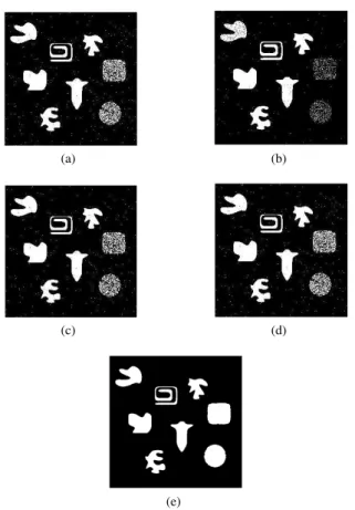
To demonstrate the robustness of the proposed method, we have estimated the number of clusters and centroids in synthetic images contaminated with additive gaussian noise.

The segmentation result in Fig. 3(b) was accomplished by applying the Otsu’s method and the similarity measure reached Sr = 97.56%. The proposed method estimated the clusters

and we assumed the threshold value as the minimum valley between two adjacent centroids. Moreover, it identified two clusters with a thresholdT = 124, and the segmentation result

(a)

(b) (c)

Fig. 3. Segmentation results: (a) noisy image, (b) Otsu’s method result (T = 126_{) and (c) proposed method result (}T = 124_).

achieved Sr = 98.10% which denotes a good matching

be-tween the segmented regions and the reference ones. Fig. 3(c) illustrates this segmentation result.

Fig. 4 depicts an image processed similarly, and for which our method detected two dominant clusters and estimated their centroid values (76; 153). Fig. 5 shows the clusters and centroids.

Fig. 6 illustrates the results of segmentation methods applied to the noisy image presented in Fig. 4. The Otsu’s threshold wasT = 113and the result (Fig. 6(a)) reachedSr= 79.22%.

Fig. 6(b) shows the classical K-means result and according to Sr= 71.72%value and visual analysis, this method performed

worse than the others.

Fig. 6(c) to Fig. 6(e) correspond to results from the thresh-olding (Sr = 82.98%), K-means (Sr = 84.02%) and level

set (Sr = 99.25%) algorithms, respectively. Regarding our

method, the result comprised regions with a foreground cluster (in white) and centroid value equal to153, and a background cluster (in black) with centroid equal to76.

(16)

0 50 100 150 200 250 300 0

5000 10000

Noisy Image Histogram

0 50 100 150 200 250 300

0 5000 10000

Detected Clusters

0 50 100 150 200 250 300

0 5000 10000

Clusters Centroids

Fig. 5. Detected clusters in noisy image of fig. 4(top to down) noisy image histogram, detected clusters (*) and its centroids (◦).

(a) (b)

(c) (d)

(e)

Fig. 6. Segmentation results of noisy image in Fig. 4: (a) Otsu’s thresholding result, (b) Classical K-means result, and (c)-(e) results by using the proposed method for cluster estimation, (in sequence): thresholding, K-means and level set algorithms.

V. CONCLUDINGREMARKS

In this paper, we proposed an approach to detect clusters that improved the performance of segmentation techniques and solved the uncertainty regarding the number of clusters and centroid parameters. Three segmentation methods

(threshold-ing, K-means and level set) which rely on these parameters were applied to noisy images in order to assess our multiscale approach for cluster estimation. It is noteworthy that the segmentation results of noisy images proved the effectiveness of proposed method to detect clusters in plain histograms.

The thresholding results obtained with the proposed method and Otsu’s method achieved high accuracy values, as the similarity measure Sr indicated. Thus, we conclude from the

experiments that the proposed approach is simple and effective for cluster estimation.

From the segmentation results of the K-means and level set algorithms using the proposed method, we conclude that the it improved their performance and, thus, it is promising for cluster estimation.

Moreover, further work will investigate the applicability of the proposed method for multiple cluster detection (> 2). A multiphase level set implementation should also be investi-gated with multiple clusters.

ACKNOWLEDGMENT

Author woulds like to thank FUNCAP by financial support (#P JP72000910100/12) and CNPq (#301264/2013−9).

REFERENCES

[1] C.-H. Lin, C.-C. Chen, H.-L. Lee, and J.-R. Liao, “Fast k-means algorithm based on a level histogram for image retrieval,”Expert Systems with Applications, vol. 41, pp. 3276–3283, 2014.

[2] Y. Wang, S. Xiang, C. Pan, L. Wang, and G. Meng, “Level set evolution with locally linear classification for image segmentation,” Pattern Recognition, vol. 46, pp. 1734–1746, 2013.

[3] G. Thomas, D. Flores-Tapia, and S. Pistorius, “Histogram specification: A fast and flexible method to process digital images,”IEEE Transactions on Instrumentation and Measurement, vol. 60, no. 5, pp. 1565–1578, May 2011.

[4] H. Yao, Q. Duan, D. Li, and J. Wang, “An improved k-means clustering algorithm for fish image segmentation,” Mathematical and Computer Modelling, vol. 58, pp. 790–798, 2013.

[5] E. Hadjidemetriou, M. Grossberg, and S. Nayar, “Multiresolution his-tograms and their use for recognition,”IEEE Transactions on Pattern Analysis and Machine Intelligence, vol. 26, no. 7, pp. 831–847, July 2004.

[6] A. Z. Arifin and A. Asano, “Image segmentation by histogram thresh-olding using hierarchical cluster analysis,”Pattern Recogn. Lett., vol. 27, no. 13, pp. 1515–1521, 2006.

[7] J. Puzicha, T. Hofmann, and J. M. Buhmann, “Histogram clustering for unsupervised segmentation and image retrieval,”Pattern Recognition Letters, vol. 20, pp. 899–909, 1999.

[8] G. Sita and A. G. Ramakrishman, “Wavelet domain nolinear filtering for evoked potential signal enhancement,” Computers and Biomedical Research, vol. 33, no. 6, pp. 431–446, December 2000.

[9] M. J. Shensa, “The discrete wavelet transform: Wedding the trous and mallat algorithms,”IEEE Trans. Signal Processing, vol. 40, no. 10, pp. 2464–2482, October 1992.

[10] P. Perona and J. Malik, “Scale-space and edge detection using anisotropic diffusion,” IEEE Transactions on Pattern Analysis and Machine Intelligence, vol. 12, no. 7, pp. 629–639, Jul 1990.

[11] R. C. Gonzalez and R. E. Woods,Digital Image Processing, 2nd ed. New Jersey: Prentice Hall, January 2002.

[12] J. A. Sethian,Level Set Methods and Fast Merging Methods: Evolving Interfaces in Computational Geometry, Fluid Mechanics, Comput. Vision and Materials Science, 1st ed. Cambridge: Cambridge University Press, 1999.

[13] A. Mitiche and I. B. Ayed,Variational and Level Set Methods in Image Segmentation. Berlin: Springer-Verlag, 2010.