Abstract—A new procedure for representation of elastic constant tensor in terms of its orthonormal decomposed parts is presented. Form invariants and orthonormalized basis elements are used to generate this decomposition method. Numerical examples from various engineering materials serve to illustrate and verify the decomposition procedure. The norm concept of elastic constant tensor and norm ratios are used to study the anisotropy of these materials. It is shown that this method allows to investigate the elastic and mechanical properties of an anisotropic material possessing any material symmetry and determine anisotropy degree of that material. For a material given from an unknown symmetry, it is possible to determine its material symmetry type by this method.
Index Terms— elastic constant tensor, decomposition, form invariant, orthonormalized basis elements, norm, material symmetry type.
I. INTRODUCTION
NISOTROPIC materials become the material of choice in a variety of engineering applications in the last century. Many materials are anisotropic and inhomogeneous due to the varying composition of their constituents. For instance, polycrystalline materials generally show an elastic anisotropy due to texture and the anisotropy of single crystallites. The polycrystalline and composite materials which show high anisotropy are used in many applications in industry. Everyday passed, the number of anisotropic materials is increasing by the addition of man-made anisotropic single crystals and technologically developed anisotropic materials. In order to understand the physical properties of the anisotropic materials, use of tensors by decomposing them is important. Tensors are the most significant mathematical entities to describe direction dependent physical properties of solids and the tensor components characterizing physical properties which must be specified without reference to any coordinate system.
The constitutive relation for linear anisotropic elasticity, defined by using stress and strain tensors, is the generalized Hooke's law [1]
.
kl ijkl
ij
C
(1)Manuscript received November 01, 2011.
Ç. Dinçkal is with the Civil Engineering Department (Engineering-3 Block (1.floor), Room: B-3 Block/ 120), Çankaya University, New
Campus, Eskişehir Road, 29.km, 06810, Yenimahalle/ANKARA/Türkiye
(phone:+90-312-233-1405; fax:+90-312-233-1026; e-mail: [email protected]).
This formula demonstrates the well known general linear relation between the stress tensor whose components are
ij
and the strain tensor (symmetric second rank tensor) whose components are
kl.
C
ijklare the components of elastic constant tensor (elasticity tensor)C
ijkl satisfies three important symmetry restrictions. These are,
klij ijkl ijlk ijkl jikl
ijkl
C
C
C
C
C
C
(2)which follow from the symmetry of the stress tensor, the symmetry of the strain tensor and the elastic strain energy. These restrictions reduce the number of independent elastic constants Cijklfrom 81 to 21. Consequently, for anisotropic materials (with triclinic symmetry) the elastic constant tensor has 21 independent components.
The indices are abbreviated according to the replacement rule given in the following TABLE [1]:
TABLEI
ABBREVIATION OF INDICES FOR FOUR AND DOUBLE INDEX NOTATIONS
four index notation 11 22 33 23, 32 13, 31 12, 12
double index notation 1 2 3 4 5 6
In literature, the works for orthonormal decomposition of any rank tensors can be summarized as; it was first proposed by [2], developed by [3] who gave name as integrity basis treated the strain energy function as a polynomial in the strain components and lead to determination integrity basis for invariant functions of the strain components for each one of the 32 crystallographic point groups. Using the integrity basis, orthonormal tensor basis which spans the space of elastic constants was derived. Orthonormal tensor basis is also obtained by another way which is form invariant. Reference [4] identified invariant elastic constants for each crystal class.
The purpose of the work is to develop a new decomposition method for elastic constant tensor in order to prove that a material possesses a particular symmetry type can be explained in another anisotropic symmetry.
In the present paper, the decomposition method is introduced. Next, norm concept and anisotropy degree are presented. As an application of this method, numerical examples are given from randomly selected materials. Finally, in the last section, the results of numerical analysis are discussed and conclusions pertinent to this work are stated.
An Innovative Description of Elastic Constant
Tensor Based upon Orthonormal
Representations
Çiğdem Dinçkal
II. DECOMPOSITION PROCESS
In analyzing the elastic and mechanical properties of anisotropic linear materials, elastic constant tensor is required to make up a linear constitutive relation between stress and strain tensors, each of which represents some directly detectable and measurable effect in the material (Recall Hooke's law, given in (1)). Elastic constant tensor is introduced in specification of physical properties for many anisotropic materials. Decomposition of the elastic constant tensor into orthonormal parts, offer not only valuable insight into the tensor structure but also simplify immensely the calculations of sums, products, inverses and inner products. The decomposition method developed can be carried out for materials possessing symmetry classes such as isotropic, cubic, transversely isotropic, tetragonal (classes:
4
mm
,
, 2
4 m
422
,
4/mmm), trigonal (classes:32
,
3m
,
3
m
), orthorhombic and triclinic [1]. In this work, materials possessing isotropic, transversely isotropic and orthorhombic symmetry are selected for application since important engineering materials exhibit those symmetries.For isotropic materials, an expression for the elastic constant tensor which is different from the traditional form is also presented.
A. Form Invariant
A physical property of tensor is resolved along the triads
3 2 , 1
v
,v
v
denoting the unit vectors along the material coordinate axis [4]. The symmetry properties of the material, due to the geometric or crystallographic symmetry, can be defined by the group of orthonormal transformations which transform any of these triads
a into its equivalent positions. For each of the symmetry classes selected, as reference system a rectangular Cartesian coordinate systemOxyz
is chosen, so related to the material directions
1,
,
2
3 in the material under consideration that thesymmetry of the material may be described by one or more of the transformations. Their relative orientations in the seven crystal systems are well known. Transformations in which the coefficients satisfy the orthogonality relations are called linear orthogonal transformations. In this formulation, the number of elastic constants and their values do not depend on the choice of the coordinate system. The form invariant expression for the components of elastic constant tensor, the elastic stiffness coefficients is,
abcd dl ck bj ai
ijkl
A
C
(3) Where summation is implied by repeated indices,
ai are the components of the unit vectors
a (a1,2,3) along the material direction axes.A
abcd is invariant in the sense that when the Cartesian system is rotated to a new orientation, ´ ´ ´ zy
Ox then (3) takes the following form;
abcd dl ck bj ai
ijkl
A
C
´
´
´
´
´
(4) Where
1,
2,
3 form a linearly independent basis in three dimensions but they are not necessarily always orthogonal (it is a general case). The orthogonality condition used inthis work, is a particular case for elastic constant tensor so the corresponding reciprocal triads must satisfy the following relation
ij aj
ai
(5) The expression given in (5) can be rewritten asI
T
(6)Where
I
is identity matrix which is.
1
0
0
0
1
0
0
0
1
33 32 31
23 22 21
13 12 11
(7)
Since
ij
1
(i
j
) or
ij
0
(i
j
). These are the orthogonality relations which are also defined in (5).B. Orthonormalized Basis Elements
Form invariant is the necessary step in constructing orthonormal tensor basis of elasticity tensors. By appropriate use of
ij , elements of the orthonormal tensor basis can be constructed for each symmetry types [5]. Furthermore symmetry in crystal means simply invariance of the properties with respect to the transforms of some subgroup of the orthogonal group, whereas the properties of an isotropic medium are invariant with respect to all the transforms of the orthogonal group. In other words, it explains the form ofC
ijkltensor for any isotropic medium and it is invariant with respect to the all transforms of the orthogonal group. However there is a unique tensor that is not affected by all orthogonal transforms, it is a unique tensor, apart from a scalar factor, soC
ijkl can be expressed as combinations of the components
ij of that tensor with certain coefficients. There are only three different such combinations which contain four subscriptsi
,
j
,
k
,
l
namelykl ij
,
ik
jl,
il
jk[5]. Because of the symmetry of,
ijkl
C
i
andj
are permuted. So the elements takes the new form;
ij
kl and
ik
jl
il
jk. For other symmetry types, these elements are used in a suitable form, when constructing orthonomalized basis. Form-invariant expression of isotropic symmetry is formed by the following two basis elements:jk il jl ik kl
ij
,
(8)So, the decomposition of
C
ijkl for triclinic system with no elastic symmetries is given in terms of its orthonormalized basis elements as),
...
(
,
)
,
(
C
A
A
K
I
XXI
C
ijklK ijklKK
ijkl
(9)Where
(
C
,
A
ijklK)
represents the inner product ofC
ijkl)], ( 2 ) [( 3 1 ) ,
(C AijklI C11C22C33 C12C13C23
)], ( 2 ) ( 6 ) ( 2 [ 5 3 1 ) , ( 23 13 12 66 55 44 33 22 11 C C C C C C C C C A C II ijkl )], ( 3 [ 6 1 ) ,
(C AIII C33 C11 C22 C33
ijkl
)], ( 2 3 3 [ 3 1 ) ,
(C AIV C13 C23 C12 C13 C23
ijkl
)], ( 2 ) ( 4 ) ( 2 [ 30 1 ) , ( 23 13 12 66 55 44 33 22 11 C C C C C C C C C A
C ijklV
], 2 [ 3 2 ) ,
(C AVI C44 C55 C66
ijkl [ ],
2 1 ) ,
(C AVII C11 C22
ijkl
],
[
)
,
(
C
A
ijklVIII
C
13
C
23(
C
,
A
IX)
2
[
C
44C
55],
ijkl
,
2
2
)
,
(
C
A
C
46X
ijkl
(
C
,
A
)
2
C
35,
XI
ijkl
(
C
,
A
)
2
C
15,
XII ijkl
,
2
)
,
(
C
A
ijklXIII
C
25 (C,A ) 2 2C45,(C,A ) 2C16, XVijkl XIV
ijkl
,
2
)
,
(
C
A
ijklXVI
C
26 (C,A ) 2C36,(C,AXVIII) 2 2C56, ijklXVII
ijkl
, 2 ) ,
(C AXIX C24
ijkl (C,A ) 2C34,(C,A ) 2C14.
XXI ijkl XX
ijkl (10)
Here, elastic constants are given in Voigt notation.
C. Isotropic Materials
The form invariant expression is defined for isotropic material as [4]
)
(
ik jl il jkkl ij ijkl
C
(11)Where
and
are invariant elastic constants and they are also called Lame constants and
ijkl
ij
kl,jk il jl ik
ijkl
.The traditional form of stress-strain relation for isotropic solids can be defined asij ij
rr
ij
2
(12)It is also well known that stress tensor is decomposed into spherical and deviatoric parts and it is given as
).
3
1
(
3
1
ij rr ij ij rrij
(13)For isotropic materials, the decomposition of
C
ijklfor the isotropic system is given in terms of the orthonormalized basis elements as)
,
(
,
)
,
(
)
,
(
)
,
(
C
A
A
C
A
A
C
A
A
K
I
II
C
ijklK ijklK ijklI ijklI ijklII ijklIIK
ijkl
(14) Where
(
,
K)
ijkl
A
C
denotes the inner product ofC
ijkl and , 3 1 3 1 kl ij ijkl I ijklA (3 2 )
5 6 1 ijkl ijkl II ijkl
A which are
orthonormalized basis elements for isotropic system. The inner products are
)], ( 2 ) [( 3 1 ) ,
(C A C11 C22 C33 C12 C13 C23
I
ijkl (15)
)]. ( 4 ) ( 12 ) ( 4 [ 5 6 1 ) ,
(CA C11 C22 C33 C44 C55 C66 C12 C13 C23
II
ijkl
(16) Equation (14) denotes the new representation of elastic constant tensor for isotropic symmetry which is not in literature.
D. Transversely Isotropic Materials
The form invariant expression for transversely isotropic materials [4] ijkl ijkl ijkl ijkl ijkl ijkl
C
1
2
3
4
5
(17) Where
ijkl
3i
3j
3k
3l,
ijkl
ij
k3
l3
i3
j3
kl and
ijkl
(
i2
j3
i3
j2)(
k2
l3
k3
l2)
(
i1
j3
i3
j1)(
k1
l3
k3
l1).
,
1
2,
3,
4 and
5 are invariant elastic constants for transversely isotropic system. The decomposition ofijkl
C
for transversely isotropic system is given in terms of the orthonormalized basis elements asV ijkl V ijkl IV ijkl IV ijkl III ijkl III ijkl II ijkl II ijkl I ijkl I ijkl ijkl
A
A
C
A
A
C
A
A
C
A
A
C
A
A
C
C
)
,
(
)
,
(
)
,
(
)
,
(
)
,
(
(18)Where
(
15
),
5
6
1
ijkl ijkl ijkl III ijklA
),
5
15
9
(
12
1
ijkl ijkl ijkl ijkl IV ijklA
)
3
2
(
4
1
ijkl ijkl ijkl ijkl ijkl V ijklA
Which are orthonormalized basis elements for transversely isotropic system.Since first two orthonormalized basis elements of transversely isotropic system are the same as isotropic symmetry, inner products are also identical, the other inner products for transversely isotropic system are
], 4 4 4 2 2 2 12 3 3 [ 5 6 1 ) , ( 66 55 44 23 13 12 33 22 11 C C C C C C C C C A C III ], 4 4 4 8 8 10 3 3 [ 12 1 ) , ( 66 55 44 23 13 12 22 11 C C C C C C C C A C IV ]. 4 4 4 2 [ 4 1 ) ,
(C AV C11C22 C12 C44 C55 C66 (19) E. Orthorhombic Materials
). )(
( i2 j3 i3 j2 k2 l3 k3 l2
ijkl
,
1
2,
3,
4,
5,
6,
7,
8 and
9 are invariant elastic constants for orthorhombic system. The decomposition ofijkl
C
for orthorhombic system is given in terms of its orthonormalized basis elements as)
...
(
,
)
,
(
C
A
A
K
I
IX
C
ijklKK ijkl K
ijkl
(21)Where
),
3
2
(
2
2
1
ijkl ijkl ijkl ijkl ijkl ijkl VI ijklA
),
2
1
2
1
2
(
2
1
ijkl ijkl ijkl ijkl VII ijklA
), 2 2 ( 2 1 ijkl ijkl ijkl VIII ijkl
A
(2 ),2 2 1 ijkl ijkl IX ijkl
A
which are orthonormalized basis elements for orthorhombic system. ( , K )
ijkl
A
C represents the inner product of
C
ijkl fororthorhombic symmetry and the
K
th elements,A
ijkl of the basis, since first five orthonormalized basis elements of orthorhombic system are the same as transversely isotropic symmetry, inner products are also common, the other four inner products for orthorhombic materials are], 4 2 [ 2 2 1 ) ,
(C AVI C11 C12C22 C66
], [ 2 1 ) ,
(C AVII C11C22
(
C
,
A
)
C
13C
23,
VIII
). (
2 ) ,
(C AIX C44C55
(22)
III. NUMERICAL ANALYSIS
Let us consider the decomposition of the elastic constant tensor in the following materials.
A. For an Isotropic Material
Especially textured and non-crystalline materials show isotropic symmetry. There are two independent elastic constants for isotropic symmetry which are
C
11,
C
12.
Reactor pressure vessel (RPV) steel is presented as isotropic material and the elastic coefficients in GPa (10
10dyncm2) for RPV steel are given [6] 143 . 79 0 0 0 0 0 0 143 . 79 0 0 0 0 0 0 143 . 79 0 0 0 0 0 0 001 . 277 715 . 118 715 . 118 0 0 0 715 . 118 001 . 277 715 . 118 0 0 0 715 . 118 715 . 118 001 . 277 ij C (23)
By using the formula given in (14), inner products are calculated as
.
94
.
353
)
,
(
,
431
.
514
)
,
(
C
A
I
C
A
II
(24)The symmetric fourth rank tensor for RPV steel can be represented in the form
II ijkl I
ijkl
ijkl A A
C 514.431 353.94 (25)
Regarding (25), elastic constant tensor of RPV can be decomposed as 143 . 79 0 0 0 0 0 0 143 . 79 0 0 0 0 0 0 143 . 79 0 0 0 0 0 0 524 . 105 762 . 52 762 . 52 0 0 0 762 . 52 524 . 105 762 . 52 0 0 0 762 . 52 762 . 52 524 . 105 0 0 0 0 0 0 0 0 0 0 0 0 0 0 0 0 0 0 0 0 0 477 . 171 477 . 171 477 . 171 0 0 0 477 . 171 477 . 171 477 . 171 0 0 0 477 . 171 477 . 171 477 . 171 ij C (26)
B. For a Transversely Isotropic Material
Most textured and non-crystalline materials exhibit transversely isotropic symmetry. There are five independent elastic constants for transversely isotropic symmetry which are
C
11,
C
12,
C
13,
C
33,
C
44.
Polystyrene is presented as a transversely isotropic material and the elastic coefficients in GPa for Polystyrene are given [7] 225 . 1 0 0 0 0 0 0 30 . 1 0 0 0 0 0 0 30 . 1 0 0 0 0 0 0 70 . 5 75 . 2 75 . 2 0 0 0 75 . 2 20 . 5 75 . 2 0 0 0 75 . 2 75 . 2 20 . 5 ij C (27)
By applying the formula given in (18), inner products can be computed as
. 15 . 0 ) , ( , 05 . 0 ) , ( , 4025 . 0 ) , ( , 7616 . 5 ) , ( , 87 . 10 ) , ( V IV III II I A C A C A C A C A C (28) The elastic constant tensor for Polystyrene can be decomposed as V ijkl IV ijkl III ijkl II ijkl I ijkl ijkl A A A A A C 15 . 0 05 . 0 4025 . 0 7616 . 5 87 . 10 (29)
From (29), isotropic and transversely isotropic parts of Polystyrene are constructed as
II ijkl I
ijkl
A
A
I
10
.
87
5
.
7616
(30)V ijkl IV
ijkl III
ijkl
A
A
A
TI
0
.
4025
0
.
05
0
.
15
(31) By adding (30) and (31), elastic constant tensor of RPV can be represented as 2883 . 1 0 0 0 0 0 0 2883 . 1 0 0 0 0 0 0 2883 . 1 0 0 0 0 0 0 3411 . 5 7644 . 2 7644 . 2 0 0 0 7644 . 2 3411 . 5 7644 . 2 0 0 0 7644 . 2 7644 . 2 3411 . 5 ij C . 063 . 0 0 0 0 0 0 0 0117 . 0 0 0 0 0 0 0 0117 . 0 0 0 0 0 0 0 36 . 0 0133 . 0 0133 . 0 0 0 0 0133 . 0 14 . 0 0133 . 0 0 0 0 0133 . 0 0133 . 0 14 . 0 (32)
C. For an Orthorhombic Material
orthorhombic symmetry. There are nine independent elastic constants for orthorhombic symmetry which are
.
,
,
,
,
,
,
,
,
22 33 12 13 23 44 55 6611
C
C
C
C
C
C
C
C
C
Olivine ispresented as an orthorhombic material and the elastic coefficients in GPa for Olivine are given [8]
49 0 0 0 0 0 0 62 0 0 0 0 0 0 60 0 0 0 0 0 0 272 56 60 0 0 0 56 160 66 0 0 0 60 66 192 ij C (33)
By employing the formula given in (21), inner products are calculated as
, 18 ) , ( , 67 . 8 ) , ( , 461 . 86 ) , ( , 73 . 284 ) , ( , 33 . 329 ) ,
(CAI CAII CAIII CAIV CAV
. 83 . 2 ) , ( , 4 ) , ( , 6 . 22 ) , ( , 49 . 8 ) ,
(C AVI C AVII C AVIII C AIX
(34) The symmetric fourth rank tensor for Olivine can be represented in the form
IX ijkl VIII ijkl VII ijkl VI ijkl V ijkl IV ijkl III ijkl II ijkl I ijkl ijkl A A A A A A A A A C 83 . 2 4 6 . 22 49 . 8 18 67 . 8 461 . 86 73 . 284 33 . 329 (35) From (35), isotropic and transversely isotropic, tetragonal and orthorhombic parts of Olivine are constructed as
II ijkl I
ijkl A
A
I 329.33 284.73 (36)
V ijkl IV ijkl III
ijkl A A
A
TI86.461 8.67 18 (37)
VI ijkl
A
Tet8.49 (38)
IX ijkl VIII
ijkl VII
ijkl A A
A
O22.6 4 2.83 (39) By adding (36), (37), (38) and (39), elastic constant tensor of Olivine can be denoted as
7 . 11 0 0 0 0 0 0 7 . 2 0 0 0 0 0 0 7 . 2 0 0 0 0 0 0 3 . 77 3 . 9 3 . 9 0 0 0 3 . 9 7 . 21 7 . 1 0 0 0 3 . 9 7 . 1 7 . 21 7 . 63 0 0 0 0 0 0 7 . 63 0 0 0 0 0 0 7 . 63 0 0 0 0 0 0 7 . 194 3 . 67 3 . 67 0 0 0 3 . 67 7 . 194 3 . 67 0 0 0 3 . 67 3 . 67 7 . 194 ij C . 0 0 0 0 0 0 0 1 0 0 0 0 0 0 1 0 0 0 0 0 0 0 2 2 0 0 0 2 16 0 0 0 0 2 0 16 3 0 0 0 0 0 0 0 0 0 0 0 0 0 0 0 0 0 0 0 0 0 0 0 0 0 0 0 3 3 0 0 0 0 3 3 (40)
IV. THE NORM CONCEPT AND ANISOTROPY DEGREE
Norm is an invariant of the material. There are many types of norm in literature. Those norms are Euclidean, Riemannian, log-Euclidean, Taxicab, infinity, uniform, zero and so on. These norms are used in different fields of science and engineering. For instance, zero norm is related with machine learning and optimization. Log-Euclidean norm is a measure for tensors such as symmetric positive-definite matrices in medical imaging, modeling of anatomical variability i.e. human brain variability and Riemannian and log-Euclidean norms are used to find the shortest distance between an elasticity tensor of arbitrary symmetry and an elasticity tensor of lower symmetry. [9] These two norms are effective when elastic compliance tensor is considered. Since the most appropriate and reliable norm for elastic constant tensor is Euclidean norm in literature, Euclidean norm is used for computations as a
measure in this work. Comparison of magnitudes of the Euclidean norm gives valuable information about the origin of the physical property under examination. Euclidean norm also represents the stiffness effect in the material like fiber-reinforced composites.
Euclidean norm of a Cartesian tensor is defined as the square root of the contracted product over all the indices with itself, which is given as follows
2 1
} {Cijkl...Cijkl... C
N (41)
Since the basis constructed in this thesis is orthonormal and
C
ijkl... is in the space spanned by that orthonormal basis} { K
A , it is straightforward to see that, now the norm
2 1 } ) , ( { ijklK 2
K A C C
N (42)
The norm of nearest isotropic tensor, denoted by
C
iiklo,
ofijkl
C
is therefore) , ( , } ) , ( { 2 1 2 II I K A C C N K ijkl o I K o
i
(43)
In similar way, with respect to the tensorCijkl, the nearest tensors of other symmetry classes within the class spanned by the basis { K}
A can be read off from the representation and their norms may be computed according to (42). By using the norms, the nearest isotropic tensors of lower symmetries such as cubic, transversely isotropic, tetragonal, trigonal and orthorhombic can be found via the following formula [3]
C C
C o
o
(44)
Where
o is a scalar constant independent of the rotation of the axes. It is a measure of `nearness' of the nearest isotropic tensor.It is obvious that the anisotropy of the material, for instance, the symmetry group of the material and the anisotropy of the measured property depicted in the same materials may be quite different. Clearly, the property tensor must show, at least, the symmetry of the material. For instance, a property which is measured in a material can almost be isotropic but the material symmetry group itself may have very few symmetry elements. We know that, for isotropic materials, the elastic constant tensor has two scalar (isotropic) parts, so the norm of the elastic constant tensor for isotropic materials depends only on the norm of the scalar parts, i.e., NNi. so, the ratio
N
i/
N
1
forisotropic materials. For cubic materials, the elastic constant tensor has the same two parts that consisting the isotropic symmetry and a third which is designated as the anisotropic part, hence we define two ratios:
N
i/
N
for the isotropic parts andN
a/
N
for the anisotropic part. For lower symmetry type materials such as transversely isotropic, tetragonal, trigonal and orthorhombic, the elastic constant tensor additionally contains more anisotropic parts, so we can defineN
a/
N
for all the anisotropic parts.asses and compare the anisotropy degree of a material property as a whole.
The following significant notes are taken into account when we have evaluated the computed results in following tables. These notes are:
1. It can be used as a parameter representing and comparing the overall effect of a certain property of anisotropic materials of the same or different symmetry. If the norm value of a material is large, it has more effective property than the other materials of the same symmetry type.
2. When
N
iis the largest among norms of the decomposed parts, if the norm ratio Ni/N is closer to one, the material property is closer to isotropic.3. When
N
i is not the largest or not present, norm of the other parts can be used as a criterion. But in this case the situation is reverse; if the norm ratio value is larger than the others, the material property is more anisotropic.In following sections, several examples from transversely isotropic and orthorhombic symmetries are presented.
A. Materials from Transversely Isotropy
Elastic constants of transversely isotropic materials are given in TABLE II. The units are in GPa.
TABLEII
ELASTIC CONSTANT DATA OF TRANSVERSELY ISOTROPIC MATERIALS
For transversely isotropic materials, the norm and norm ratios,
o(the anisotropy degrees) are computed in order to determine which one is close to isotropy or anisotropy. The results for norm, norm ratios and the measure of `nearness' of the nearest isotropic tensor are presented in the following TABLE.TABLEIII
THE NORM AND NORM RATIOS (THE ANISOTROPY DEGREES) FOR TRANSVERSELY ISOTROPIC MATERIALS
From TABLE III, it is seen that the ratio
N
i/
N
gives the same result for hardened and normal tool steel which is equal to1
and the results for
o is close to each other. Buto
of normal tool steel is smaller than
oof hardened tool steel which shows that normal tool steel is more isotropic than the hardened one. The same case is also proved by comparing theN
a/
N
for both tool steel type. The larger ratioN
a/
N
and,
o
the more anisotropic property exist for a transversely isotropic material and in reverse manner, the smaller ratioN
i/ N
,
a transversely isotropic materialpossesses the more anisotropic property. So Zinc is the most anisotropic material among the other transversely isotropic materials.
B. Materials from Orthorhombic Symmetry
Elastic constants of orthorhombic materials are presented in TABLE IV. The units are in GPa.
TABLEIV
ELASTIC CONSTANT DATA OF ORTHORHOMBIC MATERIALS
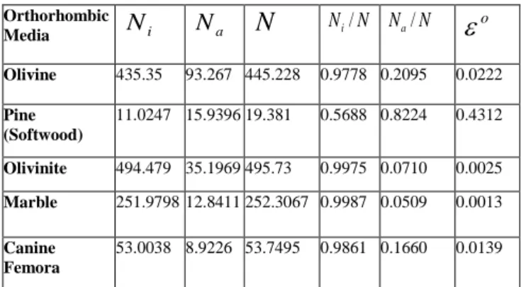
The norm and norm ratios,
o(the anisotropy degrees) for orthorhombic materials are calculated in order to determine the effect of anisotropy in other words which one is more anisotropic or isotropic. The results for norm, norm ratios and the measure of `nearness' of the nearest isotropic tensor are summarized in TABLE V.TABLEV
THE NORM AND NORM RATIOS (THE ANISOTROPY DEGREES) FOR ORTHORHOMBIC MATERIALS
In TABLE V, by taking into account the effect of the norm ratios;
N
i/ N
,
N
a/
N
and
o,
it is obvious that marble is an orthorhombic material that possesses the most isotropic effect among the other orthorhombic materials with theOrthor-
hombic
Media
11
C
C
12C
13C
22C
23C
33C
44C
55C
66Olivine [8] 192 66 60 160 56 272 60 62 49
Pine(Soft-wood) [14]
1.24 0.74 0.76 17.1 0.94 1.79 1.18 0.079 0.91
Olivinite[10] 232 93 92 210 82 199 73.3 70.9 68.6
Marble [10] 119 51 52 110 47 104 29.7 30.7 32.6
Canine
femora [15]
19 9.73 11.9 22.2 11.9 29.7 6.67 5.67 4.67
Transversely isotropic
Media
C
11C
12C
13C
33C
44Polystyrene [7] 5.20 2.75 2.75 5.70 1.30
Hardened tool steel [10] 277 113 112 272 80.3
Zinc(Zn)[11] 165 31.1 50 61.8 39.6
Cadmium[12] 116 42 41 50.9 19.6
Normal tool steel[13] 289 116 117 284 84.5
Transversely isotropic Media
i
N
N
aN
Ni/NN
a/
N
oPolystyrene 12.2996 0432 12.31 0.9994 0.0351 0.000617
Hardened tool steel
617.745 5.257 617.768 1.000 0.0085 0.000036
Zinc(Zn) 301.619 98.510 317.298 0.9506 0.3105 0.049400
Cadmium 211.340 60.330 219.7819 0.9616 0.2745 0.038400
Normal tool steel
645.282
5.367 645.3038 1.000 0.0083 0.000035
Orthorhombic
Media
N
iN
aN
Ni/N Na/N
oOlivine 435.35 93.267 445.228 0.9778 0.2095 0.0222
Pine (Softwood)
11.0247 15.9396 19.381 0.5688 0.8224 0.4312
Olivinite 494.479 35.1969 495.73 0.9975 0.0710 0.0025
Marble 251.9798 12.8411 252.3067 0.9987 0.0509 0.0013
Canine Femora
largest value for ratio Ni/N and the smallest value for
o
.Pine, which is a softwood, exhibits the most anisotropic property among the others with the largest value for ratio
N
N
a/
and
o .V. RESULTS AND CONCLUSION
This decomposition method for elastic constant tensor have many applications in various subjects of science (atomic and molecular physics and the physics of condensed matter) and engineering such as decomposition of wood elastic constant tensor in structural engineering or representation of olivine elastic constant tensor in geophysical applications. In the mechanics of continuous media, for instance, in elasticity studies; the stress and strain tensors are decomposed into spherical (hydrostatic) and deviatoric parts each of which have important meanings.
Moreover, for very valuable materials (diamonds, quartz) used in mining, it is difficult to measure its elastic constants because of its small samples. Applying this decomposition procedure, it is possible to specify the elastic constants of these types of materials.
Representation of elastic constant tensor in terms of its orthonormal parts by this method provides a deeper understanding about elastic and mechanical behavior of anisotropic materials. It also has more significant effects on many applications in different fields such as:
1) Calculation of norm and norm ratios for assessing and comparing the anisotropic properties of materials.
2) Examining the material symmetry types in detail, 3) Observing a material which possesses a particular symmetry type can be explained in another anisotropic symmetry.
4) Determination of materials possessing same crystal symmetry type which are highly anisotropic or close to isotropy,
5) Understanding the mechanical and elastic behavior of natural composites such as Bone and Wood types.
REFERENCES
[1] J. F. Nye, Physical Properties of Crystals, Their Representation by Tensors and Matrices, Oxford University Press, 1964, pp.131-149. [2] D. C. Gazis, Tadjbakhsh and R. A. Toupin, „„The elastic tensor of
given symmetry nearest to an anisotropic elastic tensor‟‟, Acta Crsyt., vol. 16, pp. 917-922, 1963.
[3] Yih-O Tu, „„The decomposition of an anisotropic elastic tensor‟‟
Acta Cryst., A24, pp. 273-282, 1968.
[4] T. P. Srinivasan, S. D. Nigam, „„Invariant elastic constants for
crystals‟‟, Journal of Mathematics and Mechanics, vol. 19, pp. 411-420, 1969.
[5] F. I. Fedorov, Theory of Elastic Waves in Crystals, Plenum, New
York, 1968.
[6] Cheong,Yong-Moo, „„Dynamic elastic constants of weld HAZ
of SA 508 CL.3 steel using resonant ultrasound spectroscopy‟‟,
Korea Atomic Energy Research Institute, Korea, 1999.
[7] A. Wright, C. S. N. Faraday, E. F. T. White, „„Elastic constants of
oriented glassy polymers‟‟, Journal of Physics D- Applied Physics, vol. 4, pp. 2002, 1971.
[8] S. Chevrot, J. T. Browaeys, “Decomposition of the elastic tensor and
geophysical applications‟‟, Geophys. J. Int., vol. 159, pp. 667-678, 2004.
[9] M. Moakher, A. N. Norris, “The closest elastic tensor of arbitrary symmetry to an elasticity tensor of lower symmetry”, Journal of Elasticity, vol. 85, pp. 215-263, 2006.
[10] K. S. Aleksandrov, T. V. Ryzhove and B. P. Belikov, Izv. Akad. Nauk. SSSR. Ser. Geol., vol. 6, pp. 17, 1968.
[11] D. P. Singh, S. Singh and S. Chendra, Indian J. Phys., A 51, pp. 97,
1977.
[12] Y. Li, Physics Status Solidi a, vol. 38, pp. 171, 1976.
[13] E. P. Papadakis , “ Ultrasonic study of simulated crystal symmetries in polycrystalline aggregates‟‟, IEEE. Trans. Sonic. Ultrasonic, vol. 11, pp. 19, 1964.
[14] R. Yamai, J Japan. Forestry Soc., vol. 39, pp.328, 1957.
[15] S. C. Cowin, W. C. Van Buskirk, “Thermodynamics restrictions on
the elastic constants of bone‟‟, Journal of Biomechanics, vol. 19, pp.