A novel calibration approach of MODIS AOD data to predict PM<sub>2.5</sub> concentrations

(1)

ACPD

11, 9769–9795, 2011

A calibration method of MODIS AOD data

to predict PM₂_.₅

H. J. Lee et al.

Title Page

Abstract Introduction

Conclusions References

Tables Figures

◭ ◮

Back Close

Full Screen / Esc

Printer-friendly Version

Interactive Discussion

Discussion

P

a

per

|

Dis

cussion

P

a

per

|

Discussion

P

a

per

|

Discussio

n

P

a

per

Atmos. Chem. Phys. Discuss., 11, 9769–9795, 2011 www.atmos-chem-phys-discuss.net/11/9769/2011/ doi:10.5194/acpd-11-9769-2011

Atmospheric Chemistry and Physics Discussions

This discussion paper is/has been under review for the journal Atmospheric Chemistry and Physics (ACP). Please refer to the corresponding final paper in ACP if available.

A novel calibration approach of MODIS

AOD data to predict PM

₂

_.

₅

concentrations

H. J. Lee1, Y. Liu2, B. A. Coull3, J. Schwartz1, and P. Koutrakis1

1

Department of Environmental Health, Harvard School of Public Health, Boston, MA 02215, USA

2

Department of Environmental and Occupational Health, Rollins School of Public Health, Emory University, Atlanta, GA 30322, USA

3

Department of Biostatistics, Harvard School of Public Health, Boston, MA 02115, USA

Received: 7 March 2011 – Accepted: 20 March 2011 – Published: 23 March 2011

Correspondence to: H. J. Lee (hlee@hsph.harvard.edu)

(2)

ACPD

11, 9769–9795, 2011

H. J. Lee et al.

Title Page

Tables Figures

◭ ◮

Back Close

Full Screen / Esc

Discussion

P

a

per

|

Dis

cussion

P

a

per

|

Discussion

P

a

per

|

Discussio

n

P

a

per

|

Abstract

Epidemiological studies investigating the human health effects of PM2.5 are suscep-tible to exposure measurement errors, a form of bias in exposure estimates, since they rely on data from a limited number of PM₂_.₅ monitors within their study area. Satellite data can be used to expand spatial coverage, potentially enhancing our ability

5

to estimate location- or subject-specific exposures to PM2.5, but some have reported poor predictive power. A new methodology was developed to calibrate aerosol optical depth (AOD) data obtained from the Moderate Resolution Imaging Spectroradiome-ter (MODIS). Subsequently, this method was used to predict ground daily PM2.5 con-centrations in the New England region. 2003 MODIS AOD data corresponding to the

10

New England region were retrieved, and PM₂_.₅concentrations measured at 26 US En-vironmental Protection Agency (EPA) PM2.5monitoring sites were used to calibrate the AOD data. A mixed effects model which allows day-to-day variability in daily PM2.5 -AOD relationships was used to predict location-specific PM₂_.₅levels. PM₂_.₅ concentra-tions measured at the monitoring sites were compared to those predicted for the

cor-15

responding grid cells. Both cross-sectional and longitudinal comparisons between the observed and predicted concentrations suggested that the proposed new calibration approach renders MODIS AOD data a potentially useful predictor of PM2.5 concentra-tions. Furthermore, the estimated PM2.5levels within the study domain were examined in relation to air pollution sources. Our approach made it possible to investigate the

20

spatial patterns of PM2.5concentrations within the study domain.

1 Introduction

Atmospheric aerosols originate from natural and anthropogenic emission sources. Par-ticularly, anthropogenic aerosols are considered to have major human health implica-tions, and numerous studies have reported associations between mortality and

morbid-25

(3)

ACPD

11, 9769–9795, 2011

H. J. Lee et al.

Title Page

Tables Figures

◭ ◮

Back Close

Full Screen / Esc

Discussion

P

a

per

|

Dis

cussion

P

a

per

|

Discussion

P

a

per

|

Discussio

n

P

a

per

1996; Slama et al., 2007). The PM₂_.₅health effect studies generally use PM₂_.₅ mea-surements from ground monitoring sites, but there are many regions with no ground PM2.5measurements available due to their sparse monitoring networks. This limits the ability of estimating human exposures to PM₂_.₅, which is likely to cause less reliable health effect assessments.

5

Satellite remote sensing can be used to assess PM2.5 air quality for areas where surface PM₂_.₅ monitors are not available (Di Nicolantonio et al., 2009; Engel-Cox et al., 2004; Gupta and Christopher, 2008; Gupta et al., 2006; Koelemeijer et al., 2006; Liu et al., 2004; Schaap et al., 2009; van Donkelaar et al., 2010). The most appli-cable satellite-retrieved product for estimating PM₂_.₅ concentrations is aerosol optical

10

depth (AOD), which measures the light extinction by aerosol scattering and absorption in the atmospheric column. Since the AOD reflects the integrated amount of particles in the vertical column, it has been used as an input parameter in statistical models predicting PM₂_.₅ levels. In addition to AOD values, several studies have also included other predictor parameters such as local meteorology and land use information (e.g.,

15

population density). As reported by previous studies, these parameters influence the relationship between AOD and ground-level PM₂_.₅ concentrations, thus can be used as additional predictors (Liu et al., 2005, 2007a, b, c, 2009). However, these models, developed by us and others, generally predict <60% of the variability in daily PM2.5 concentrations (Paciorek et al., 2008). Additional time-varying parameters influence

20

the PM2.5-AOD relationship, including PM2.5vertical and diurnal concentration profiles, PM optical properties, and others. Therefore, it is reasonable to expect that the re-lationship between PM₂_.₅ and AOD varies by day. In this paper we introduce a new approach to calibrate Moderate Resolution Imaging Spectroradiometer (MODIS) AOD data to accurately predict PM2.5ground concentrations.

25

(4)

ACPD

11, 9769–9795, 2011

H. J. Lee et al.

Title Page

Tables Figures

◭ ◮

Back Close

Full Screen / Esc

Discussion

P

a

per

|

Dis

cussion

P

a

per

|

Discussion

P

a

per

|

Discussio

n

P

a

per

|

2 Methods

2.1 Ground-level PM2.5data

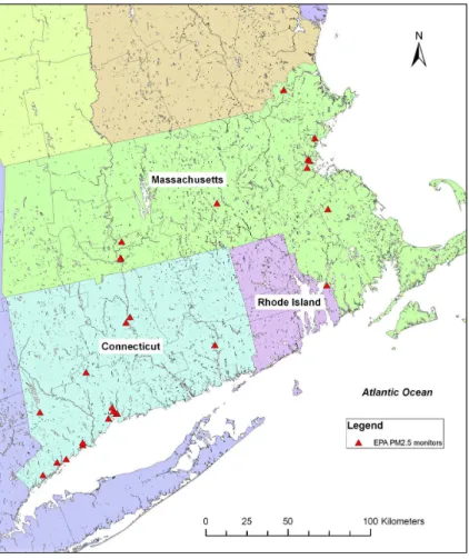
Our study region includes the States of Massachusetts (MA), Connecticut (CT), and Rhode Island (RI) in the Northeastern US. To calibrate satellite data, daily PM2.5 con-centrations measured at 26 US Environmental Protection Agency (EPA) PM2.5

mon-5

itoring sites were used (Fig. 1). For collocated monitors, we calculated the daily av-erages of the PM2.5 concentrations. Samples were collected at 15 Connecticut sites and 11 Massachusetts sites during the period 1 January through 31 December 2003. Sampling frequency differed by site including collecting samples every day, every third day, and every sixth day.

10

2.2 AOD retrieval

MODIS aboard the National Aeronautics and Space Administration (NASA)’s Earth Observing System (EOS) satellites, Terra and Aqua, was used to retrieve AOD (Col-lection 5; Level 2 aerosol product) for the year 2003. The Terra and Aqua satellites were launched in December 1999 and in May 2002, respectively. These polar-orbiting

15

satellites, operating at an altitude of approximately 700 km, provide data every one to two days under cloud-free conditions. Their sensors scan the swath of 2330 km (cross-track) by 10 km (along-track at nadir) and gather information on particle abundance once from each satellite: approximately 10:30 a.m. and 1:30 p.m. local times for Terra and Aqua, respectively. In the Collection 5 retrieval algorithm, three di_fferent channels

20

of 0.47, 0.66, and 2.12 µm are primarily employed for over-land retrievals. The chan-nels of 0.47 and 0.66 µm are used to retrieve AOD values which are interpolated to report AOD values at the wavelength of 0.55 µm, and the uncertainty of the MODIS AOD is expected to be∆AOD=±0.05±0.15×AOD over land. Furthermore, the max-imum AOD value is constrained to be 5.0, and negative AOD values down to −0.05

25

(5)

ACPD

11, 9769–9795, 2011

H. J. Lee et al.

Title Page

Tables Figures

◭ ◮

Back Close

Full Screen / Esc

Discussion

P

a

per

|

Dis

cussion

P

a

per

|

Discussion

P

a

per

|

Discussio

n

P

a

per

exposure values. More details about MODIS satellite data are reported in Remer et al. (2005) and Levy et al. (2007). Following the nominal resolution of MODIS (10 km), we created 387 grid cells of 10×10 km2covering our study region in ArcGIS (Version 9.3; ESRI). Subsequent analyses were based on these grid cells.

Since Terra and Aqua satellites retrieve AOD data at two different times each day,

5

the average of these two measurements should be used to predict daily PM2.5levels (Kaufman et al., 2000). However, there are many days where only one of the two re-trievals is available. To fully exploit the measurements of both satellites we primarily used Terra AOD data for our predictions, and for days with no Terra data, Aqua AOD measurement values were used to estimate the missing Terra values. This was

ac-10

complished by multiplying Aqua AOD measurements by an adjustment factor, which was necessary to account for diurnal variations (Green et al., 2009) and potential cali-bration differences in two satellite sensors. This factor was equal to the average Terra AOD/Aqua AOD ratio which was calculated for days where both Terra and Aqua data were available.

15

2.3 Statistical model

Since time-varying parameters such as relative humidity, PM₂_.₅ vertical and diurnal concentration profiles, and PM₂_.₅optical properties influence the PM₂_.₅-AOD relation-ship, our statistical model allows for day-to-day variability in this relationship. Further-more, we hypothesize that these time-varying parameters exhibit little spatial variability

20

and consequently the PM₂_.₅-AOD relationship varies minimally spatially on a given day over the spatial scale of our study. Therefore, a quantitative relationship between PM2.5 concentrations measured at 26 PM2.5monitoring sites and AOD values in their corre-sponding grid cells can be determined on a daily basis. A simple approach would be to calculate such PM2.5-AOD slopes separately for each day in the study. However,

25

(6)

ACPD

11, 9769–9795, 2011

H. J. Lee et al.

Title Page

Tables Figures

◭ ◮

Back Close

Full Screen / Esc

Discussion

P

a

per

|

Dis

cussion

P

a

per

|

Discussion

P

a

per

|

Discussio

n

P

a

per

|

is to use a mixed effects model with random intercepts and slopes (Fitzmaurice et al., 2004), shown by the following equations:

PM_{i j} = (α+u_j) + (β1 + vj)×AODi j + si+εi j (1)

(u_jv_j)∼N[(00),Σβ]

where PM_{i j} is the PM₂_.₅concentration at a spatial sitei on a dayj; AOD_{i j} is the AOD

5

value in the grid cell corresponding to sitei on a dayj;α anduj are the fixed and

ran-dom intercepts, respectively;β1andvj are the fixed and random slopes, respectively;

si∼N(0, σ

2

s) is the random intercept of site i; εi j is the error term at sitei on a day

j; andΣβ is the variance-covariance matrix for the day-specific random effects. In the statistical model, the AOD fixed effect represents the average effect of AOD on PM2.5

10

for all study days. The AOD random effects explain the daily variability in the PM₂_.₅ -AOD relationship. The site bias may arise since an -AOD value in a 10×10 km2 grid cell is an average optical depth in the given grid cell, while the PM2.5 concentrations measured at a given site may not be representative of the whole grid cell. Specifically, the bias can indicate spatial sites presenting high PM2.5 levels due to their locations

15

near high traffic areas. To control for the site bias, we added a site term as a ran-dom effect into the mixed effects model. It should be noted that the random estimates for the site term were omitted when estimating grid-specific PM2.5concentrations from AOD values, since AOD values are unbiased representatives of the corresponding grid cells. Because a slope cannot be estimated from a single data point, we excluded all

20

the pairs of measured PM2.5concentrations and their corresponding AOD values when there was only one pair on a given day before running the mixed effects model. This resulted in the exclusion of 29 days. Furthermore, the model prediction was examined using the root mean squared error (RMSE) between the measured and predicted PM2.5 concentrations on each day. Four sample days with RMSE>5 µg m−3 were excluded

25

(7)

ACPD

11, 9769–9795, 2011

H. J. Lee et al.

Title Page

Tables Figures

◭ ◮

Back Close

Full Screen / Esc

Discussion

P

a

per

|

Dis

cussion

P

a

per

|

Discussion

P

a

per

|

Discussio

n

P

a

per

enough to calibrate AOD data. Finally, PM₂_.₅estimates covering the whole study area were produced using the AOD calibration model described above.

To demonstrate whether the mixed effects model improved the ability of AOD to pre-dict PM₂_.₅concentrations we compared our model performance to that of a previously used model which assumes that the PM2.5-AOD relationship remains constant over

5

time (Wang and Christopher, 2003). In the previous model, measured PM2.5 concen-trations were regressed on AOD values retrieved in the corresponding grid cells as a fixed effect, establishing a single linear PM2.5-AOD relation applied to all sampling days. It is noted that the comparison of those two models was based on identical sampling days. As measures of accuracy and precision of the two models, we used

10

coe_fficient of determination (R2) and precision (% Precision) between the measured and predicted PM2.5concentrations. The precision was estimated as the square root of the mean of the squared errors, and % Precision was calculated as follows:

% Precision ₌ 100×(precision/measured mean PM₂_.₅) (2)

2.4 Model validation 15

To test this new approach we analyzed the 2003 MODIS data for MA, CT, and RI. We utilized a cross-validation (CV) method to examine whether the model is generalizable to any grid cell in the study domain. Toward this end the data of one site (test site) were separated from those of the other 25 sites (calibration sites). Subsequently, a model was developed using the data from the calibration sites. Finally, the model was used

20

to predict PM₂_.₅concentrations for the test site. This process was repeated until each of the 26 spatial sites was tested, and the measured PM2.5 concentrations were com-pared to those predicted at each site. Furthermore, Pearson correlation coefficients were used to examine the relationship between the measured and predicted concentra-tions in each site. Since time-series studies examine longitudinal associaconcentra-tions between

25

(8)

ACPD

11, 9769–9795, 2011

H. J. Lee et al.

Title Page

Tables Figures

◭ ◮

Back Close

Full Screen / Esc

Discussion

P

a

per

|

Dis

cussion

P

a

per

|

Discussion

P

a

per

|

Discussio

n

P

a

per

|

we examined the agreement between the measured and predicted annual mean PM2.5 concentration levels for each of the 26 sites, which was assessed by the correlation between the measured and predicted mean PM2.5 concentrations. This comparison is important for determining whether model predictions are reliable for cross-sectional studies, which require accurate assessment of spatial patterns in exposure.

5

2.5 PM_2.5levels in the study region

PM2.5 levels were estimated for each of the 387 grid cells. Since the AOD retrieval rate varies by location, the number of PM2.5 concentration predictions varied by grid cell. Therefore, a direct comparison among cell means would not be adequate for the investigation of the PM2.5 spatial patterns within the study domain. To minimize the

10

potential impact of varying predictions per grid cell we estimated the mean differences between the predicted grid cell and regional PM₂_.₅ concentrations for the days where grid cell predictions were available. Note that daily regional PM2.5concentrations were calculated by averaging the predicted PM2.5 concentrations for each of the grid cells. Since the number of AOD retrievals varied by day, the number of available PM₂_.₅

con-15

centrations used to estimate the daily regional average levels varied by day as well. To obtain reliable and representative regional PM2.5 concentrations we limited our es-timations to days with 50 or more grid cell predictions. Finally, the grid cell-specific PM2.5 mean differences between the grid cell and the regional PM2.5 concentrations were presented using septiles, which split the distribution of the mean differences into

20

(9)

ACPD

11, 9769–9795, 2011

H. J. Lee et al.

Title Page

Tables Figures

◭ ◮

Back Close

Full Screen / Esc

Discussion

P

a

per

|

Dis

cussion

P

a

per

|

Discussion

P

a

per

|

Discussio

n

P

a

per

3 Results and discussion

3.1 Descriptive statistics

The mean PM₂_.₅ concentrations measured at the 26 EPA PM₂_.₅ monitoring sites in 2003 are summarized in Table 1. The mean (SE) PM2.5 concentrations ranged from 9.0 (0.7) µg m−3 in Haverhill, MA (Site ID: 25-009-5005) to 17.0 (0.5) µg m−3 in New

5

Haven, CT (Site ID: 09-009-0018). The mean PM2.5 concentration at the New Haven site was exceptionally high as compared to those monitored at other sites, possibly because the site was located on a ramp connecting to interstate I-95. Many of the monitoring sites showed similar mean PM₂_.₅ concentrations. However, it should be noted that the number of samples used to estimate these means varied by site due

10

to differences in sampling frequencies among sites and missing data. Furthermore, mean (SE) daily AOD values observed for the 387 grid cells varied from 0.08 (0.02) to 0.36 (0.04). On average 67 AOD values were retrieved per grid cell which corresponds to 18% of the entire study period of 365 days.

3.2 PM_2.5prediction 15

In the mixed e_ffects model, 99 di_fferent daily PM₂_.₅-AOD relations were generated in 2003. The fixed effects of intercept and slope (AOD) were statistically significant (α=11.9,p <0.0001;β1=4.4, p=0.0049), respectively. The random effects of inter-cept and slope (AOD) varied considerably by day, with standard deviations of the daily intercepts and slopes of 8.0 and 2.3, respectively. This supports our hypothesis that

20

parameters influencing the relationship between PM2.5and AOD vary daily but not spa-tially. Therefore, it is possible to perform daily calibrations using data from the multiple PM2.5 monitoring sites in the study domain. It is noted that the daily intercepts and slopes were independent of the number of PM2.5-AOD pairs on a given day. In addi-tion, the averages of the daily intercepts and slopes were found to be 12.7 (SD₌8.7)

(10)

ACPD

11, 9769–9795, 2011

H. J. Lee et al.

Title Page

Tables Figures

◭ ◮

Back Close

Full Screen / Esc

Discussion

P

a

per

|

Dis

cussion

P

a

per

|

Discussion

P

a

per

|

Discussio

n

P

a

per

|

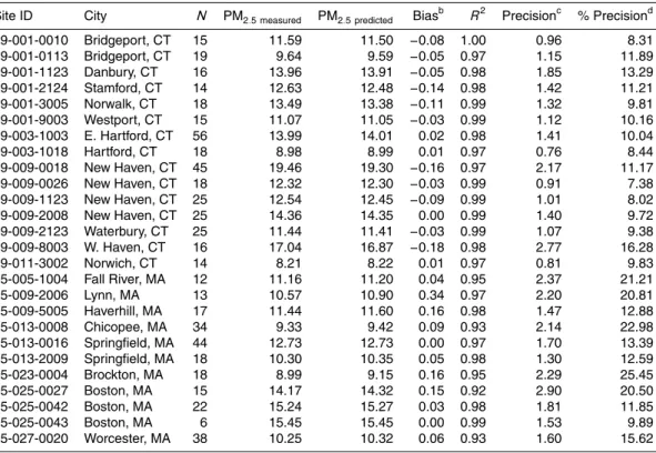
and 4.6 (SD=2.5) in warm season (15 April–14 October) and 10.1 (SD=5.4) and 3.8 (SD=1.3) in cold season (15 October–14 April), respectively. The random effect es-timates of the site term for densely populated and high traffic areas were positive as presented in Table 2. Therefore, inclusion of the site term was necessary to adjust for the site bias in our model. As shown by Table 3 and Fig. 2a, the mixed effects

5

model performed quite well. Table 3 presents the site-specific comparisons between the measured and predicted PM₂_.₅ concentrations in the mixed effects model, and the model prediction was reliable for most spatial sites (mean % Precision=13.16%, Range=7.38 to 25.45%). Moreover, Fig. 2a depicts the results of the linear regression model which was used to compare the measured and predicted daily concentrations

10

for all 26 monitoring sites (R2=0.97, slope₌0.96 (SE₌0.01), and intercept₌0.44 (SE=0.11)). In addition, Fig. 2b shows the results of the linear regression model used to compare the measured concentrations to those obtained from the CV procedure (R2=0.92, slope₌0.92 (SE₌0.01), and intercept₌0.88 (SE₌0.18)). It is noted that the predicted PM2.5 concentrations from the CV procedure were not adjusted for the

15

site bias, due to the fact that this term would not be available for location-specific pre-dictions in an epidemiological health e_ffects study. The more pronounced di_fference between the measured and predicted concentrations in Fig. 2b as compared to Fig. 2a is likely to reflect the bias. As it can be seen, both the model fit and CV test resulted in highR2, slopes close to 1, and intercepts close to 0, indicating a good agreement

20

between the measured and predicted concentrations.

In the mixed effects model, the differences between measured and predicted PM2.5 levels can be attributed to a combination of monitoring site-specific characteristics as well as PM2.5measurement and AOD retrieval errors. For instance, the monitoring site location may not be representative of a given 10×10 km2grid cell for an average

op-25

(11)

ACPD

11, 9769–9795, 2011

H. J. Lee et al.

Title Page

Tables Figures

◭ ◮

Back Close

Full Screen / Esc

Discussion

P

a

per

|

Dis

cussion

P

a

per

|

Discussion

P

a

per

|

Discussio

n

P

a

per

the measured and predicted mean PM2.5 concentrations before taking the site bias into account at the New Haven site can be explained by the fact that this site is not representative of the corresponding grid cell 10×10 km2area, and it indicates that the approach of controlling for the site bias in the mixed effects model is reasonable for the comparisons between the measured and predicted PM₂_.₅ concentrations. However,

5

considering that AOD-derived PM2.5 concentrations reflect the overall PM2.5 levels in the grid cell, the unadjusted predicted PM2.5levels may be more representative of the average population exposures to PM₂_.₅.

AOD retrieval errors due to unscreened clouds could introduce positive bias. The cur-rent cloud screening algorithm in AOD retrievals (Collection 5) effectively masks clouds,

10

but it is still possible to have AOD values a_ffected by clouds, particularly for isolated and residual clouds (Levy et al., 2007). The comparison between MODIS AOD and the Aerosol Robotic Network (AERONET) AOD (Level 2.0; within±30 min of Terra mea-surements) in Billerica could indicate days with positive bias potentially from isolated and residual clouds in the area (correlationr=0.92; slope=1.20; intercept=−0.002

15

in a linear regression model between the MODIS AOD and the AERONET AOD data) (Holben et al., 1998). Consequently, the AOD values overestimated by the clouds may cause positive bias in predicted PM2.5 concentrations. In part, PM2.5 measurement errors might cause positive or negative bias in measured PM2.5levels.

The ability of the mixed effects and linear regression models to predict PM₂_.₅

con-20

centrations was compared. For each model the predicted concentrations were re-gressed on the observed ones for each site separately (Table 4 and Fig. 3). It should be noted that the CV method produces less biased estimates than those obtained from the model fit (shown in Tables 3 and 4). The two models were compared using results from CV analyses to avoid over-fitting thus to produce more robust results. Note that

25

(12)

ACPD

11, 9769–9795, 2011

H. J. Lee et al.

Title Page

Tables Figures

◭ ◮

Back Close

Full Screen / Esc

Discussion

P

a

per

|

Dis

cussion

P

a

per

|

Discussion

P

a

per

|

Discussio

n

P

a

per

|

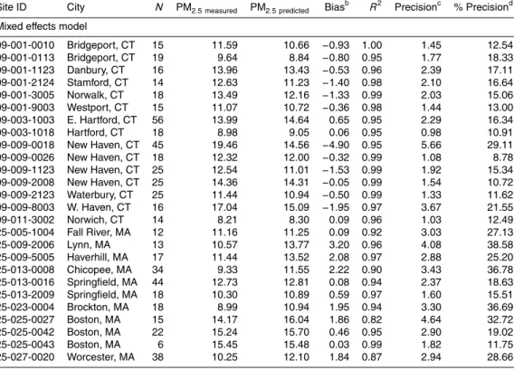
other hand, in the linear regression model, the mean variability of the measured PM2.5 explained by the predicted PM₂_.₅ was 51%, ranging from 12% in Boston, MA (Site ID: 25-025-0027) to 88% in Stamford, CT (Site ID: 09-001-2124). While the regres-sion model yielded modest and considerably varying predictability by site, our model demonstrated consistently high predictability for most of the sites. These findings

sug-5

gest that predicting PM2.5 within a domain requires the use of daily calibrations. This explains why previous investigations have not demonstrated that AOD can be a robust predictor of PM₂_.₅(Paciorek and Liu, 2009; Paciorek et al., 2008).

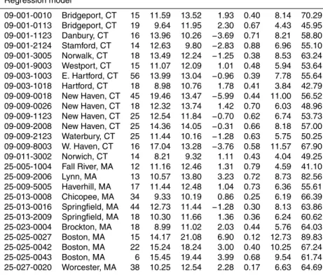
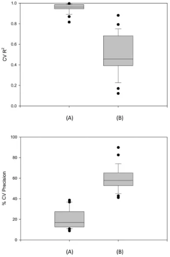
The predictive ability of our model was also compared to that of the regression model in terms of percent precision (% Precision) (Table 4 and Fig. 3). Note that this

compar-10

ison was performed using the CV results as well. Since theR2 does not reflect sys-tematic differences between the measured and predicted PM2.5levels, the measure of precision (% Precision) is necessary to better assess model performance. In the mixed e_ffects model, the % CV precision ranged from 8.8% (1.08 µg m−3) in New Haven, CT (Site ID: 09-009-0026) to 38.6% (4.08 µg m−3) in Lynn, MA (Site ID: 25-009-2006) with

15

the mean value of 20.0% (2.45 µg m−3). For the regression model the estimated mean % CV precision was 59.5% (7.40 µg m−3), varying from 41.1% (4.59 µg m−3) in Fall River, MA (Site ID: 25-005-1004) to 89.8 % (12.73 µg m−3) in Boston, MA (Site ID: 25-025-0027).

With regard to the measures of CV R2 and precision values, our model presented

20

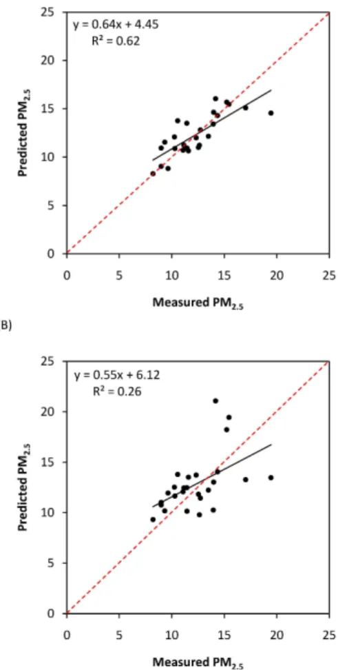
considerably higher CV R2 (0.95) and lower CV precision (20.0%, 2.45 µg m−3) than those estimated for the regression model (CV R2=0.51, % CV precision=59.5% (7.40 µg m−3)). Also, the cross-sectional comparison between the measured and pre-dicted site mean PM2.5 concentrations was performed for both models. As shown in Fig. 4, a higher correlation coefficient (R2=0.62; Pearsonr=0.79) was determined for

25

(13)

ACPD

11, 9769–9795, 2011

H. J. Lee et al.

Title Page

Tables Figures

◭ ◮

Back Close

Full Screen / Esc

Discussion

P

a

per

|

Dis

cussion

P

a

per

|

Discussion

P

a

per

|

Discussio

n

P

a

per

model can be used to produce concentration data sets reliable for both time-series and cross-sectional health e_ffect studies.

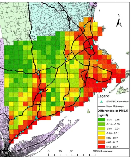
3.3 Spatial variability in PM_2.5levels

The spatial patterns of PM2.5 levels within the study domain are shown in Fig. 5. To highlight the spatial patterns, we used the mean differences between grid-specific

5

PM2.5and regional PM2.5levels, as mentioned above. Mean concentration differences varied from −0.36 to 0.87 µg m−3 (mean=0.01 µg m−3, SD=0.17 µg m−3), and were log-normally distributed, which led us to use septiles for characterizing the spatial vari-ability of PM2.5 levels in our study region. The relatively small difference between the lowest and highest values (1.23 µg m−3) compared to the one presented in

Ta-10

ble 4 can be explained by the fact that the result of Fig. 5 represented average cell concentrations which were based on the large number of overlapping days, while the large variability in average PM2.5 concentrations between sites in Table 4 was derived from the limited number of samples, used to calculate the means, which did not corre-spond to the same time period. As expected, highly populated areas such as

Bridge-15

port, New Haven, Hartford, Boston, Springfield, and Providence exhibited higher PM2.5 levels. Also, higher PM₂_.₅ levels were predicted along the major interstate highways (e.g., I-91/95) and areas with high point emission sources (e.g., power plants located in coastal cities) (US EPA, 2008). The concentration spatial patterns observed in east-ern Massachusetts were similar to those found by our previous studies (Gryparis et

20

al., 2007). Furthermore, the estimated PM2.5 levels in western Massachusetts were generally lower, which is due to the lower population density and traffic density in the area. However, it must be noted that the reported PM₂_.₅ spatial patterns may not be representative of the entire year, since AOD values are less likely to be collected during the cold season due to more frequent cloud conditions during this period. The average

25

(14)

ACPD

11, 9769–9795, 2011

H. J. Lee et al.

Title Page

Tables Figures

◭ ◮

Back Close

Full Screen / Esc

Discussion

P

a

per

|

Dis

cussion

P

a

per

|

Discussion

P

a

per

|

Discussio

n

P

a

per

|

4 Conclusions

Satellite AOD data have been increasingly used for PM2.5 air pollution studies. Re-mote sensing technologies have a great potential to expand current ground-level PM₂_.₅ monitoring networks. To date, the application of satellite data to health effect studies has been limited mostly due to the insufficient power of AOD to predict PM2.5and the

5

high frequency of non-retrieval days. We have introduced an AOD calibration method which made it possible to determine the temporal and spatial patterns of PM2.5 in a large study domain comprising the States of Massachusetts, Connecticut, and Rhode Island. An approach to PM₂_.₅ prediction for non-retrieval days will be presented in our forthcoming paper.

10

Finally, it is anticipated that future satellite technologies will provide data with finer spatial and temporal resolutions and more accurate data retrievals. In addition, the advanced capability of discriminating by aerosol species in satellite technologies will further contribute to health effect studies investigating species-specific health implica-tions. Since satellite data are readily available, PM2.5concentrations can be predicted

15

in a cost-e_ffective way. Considering the sparse ground-level PM₂_.₅ monitoring net-works, our method will help to investigate the associations between subject-specific exposures to PM2.5and their health effects.

Acknowledgements. This study was funded by the Harvard EPA PM Center (R-832416) and

the Yale Center for Perinatal, Pediatric and Environmental Epidemiology (NIH-NIEHS

R01-ES-20

(15)

ACPD

11, 9769–9795, 2011

H. J. Lee et al.

Title Page

Tables Figures

◭ ◮

Back Close

Full Screen / Esc

Discussion

P

a

per

|

Dis

cussion

P

a

per

|

Discussion

P

a

per

|

Discussio

n

P

a

per

References

Bell, M. L., Ebisu, K., and Belanger, K.: Ambient air pollution and low birth weight in Connecticut and Massachusetts, Environ. Health Perspect., 115, 1118–1125, 2007.

Di Nicolantonio, W., Cacciari, A., and Tomasi, C.: Particulate matter at surface: Northern Italy monitoring based on satellite remote sensing, meteorological fields, and in-situ samplings,

5

IEEE J. Selected Topics Appl. Earth Observ. Rem. Sens., 2, 284–292, 2009.

Dominici, F., Peng, R. D., Bell, M. L., Pham, L., McDermott, A., Zeger, S. L., and Samet, J. M.: Fine particulate air pollution and hospital admission for cardiovascular and respiratory diseases, Jama.-J. Am. Med. Assoc., 295, 1127–1134, 2006.

Engel-Cox, J. A., Holloman, C. H., Coutant, B. W., and Hoff, R. M.: Qualitative and quantitative

10

evaluation of MODIS satellite sensor data for regional and urban scale air quality, Atmos. Environ., 38, 2495–2509, 2004.

Fitzmaurice, G. M., Laird, N. M., and Ware, J. H.: Applied longitudinal analysis, New York, Wiley & Sons, 2004.

Franklin, M., Zeka, A., and Schwartz, J.: Association between PM₂_.₅and all-cause and

specific-15

cause mortality in 27 US communities, J. Expo. Sci. Environ. Epidemiol., 17, 279–287, 2007. Gent, J. F., Triche, E. W., Holford, T. R., Belanger, K., Bracken, M. B., Beckett, W. S., and

Leaderer, B. P.: Association of low-level ozone and fine particles with respiratory symptoms in children with asthma, Jama.-J. Am. Med. Assoc., 290, 1859–1867, 2003.

Gent, J. F., Koutrakis, P., Belanger, K., Triche, E., Holford, T. R., Bracken, M. B., and Leaderer,

20

B. P.: Symptoms and medication use in children with asthma and traffic-related sources of fine particle pollution, Environ. Health Perspect., 117, 1168–1174, 2009.

Green, M., Kondragunta, S., Ciren, P., and Xu, C.: Comparison of GOES and MODIS aerosol optical depth (AOD) to aerosol robotic network (AERONET) AOD and IMPROVE PM₂_.₅mass at Bondville, Illinois, J. Air Waste Manag. Assoc., 59, 1082–1091, 2009.

25

Gryparis, A., Coull, B. A., Schwartz, J., and Suh, H. H.: Semiparametric latent variable regres-sion models for spatiotemporal modeling of mobile source particles in the greater Boston area, J. R. Stat. Soc. Ser. C Appl. Stat., 56, 183–209, 2007.

Gupta, P. and Christopher, S. A.: Seven year particulate matter air quality assessment from surface and satellite measurements, Atmos. Chem. Phys., 8, 3311–3324,

doi:10.5194/acp-30

8-3311-2008, 2008.

(16)

ACPD

11, 9769–9795, 2011

H. J. Lee et al.

Title Page

Tables Figures

◭ ◮

Back Close

Full Screen / Esc

Discussion

P

a

per

|

Dis

cussion

P

a

per

|

Discussion

P

a

per

|

Discussio

n

P

a

per

|

sensing of particulate matter and air quality assessment over global cities, Atmos. Environ., 40, 5880–5892, 2006.

Holben, B. N., Eck, T. F., Slutsker, I., Tanre, D., Buis, J. P., Setzer, A., Vermote, E., Reagan, J. A., Kaufman, Y. J., Nakajima, T., Lavenu, F., Jankowiak, I., and Smirnov, A.: AERONET – A federated instrument network and data archive for aerosol characterization, Remote Sens.

5

Environ., 66, 1–16, 1998.

Kaufman, Y. J., Holben, B. N., Tanre, D., Slutsker, I., Smirnov, A., and Eck, T. F.: Will aerosol measurements from Terra and Aqua polar orbiting satellites represent the daily aerosol abun-dance and properties?, Geophys. Res. Lett., 27, 3861–3864, 2000.

Koelemeijer, R. B. A., Homan, C. D., and Matthijsen, J.: Comparison of spatial and temporal

10

variations of aerosol optical thickness and particulate matter over Europe, Atmos. Environ., 40, 5304–5315, 2006.

Levy, R. C., Remer, L. A., Mattoo, S., Vermote, E. F., and Kaufman, Y. J.: Second-generation operational algorithm: Retrieval of aerosol properties over land from inversion of Mod-erate Imaging Spectroradiometer spectral reflectance, J. Geophys. Res., 112, D13211,

15

doi:10.1029/2006JD007811, 2007.

Liu, Y., Park, R. J., Jacob, D. J., Li, Q., Kilaru, V., and Sarnat, J. A.: Mapping an-nual mean ground-level PM₂_.₅ concentrations using Multiangle Imaging Spectroradiometer aerosol optical thickness over the contiguous United States, J. Geophys. Res., 109, D22206, doi:10.1029/2004JD005025, 2004.

20

Liu, Y., Sarnat, J. A., Kilaru, V., Jacob, D. J., and Koutrakis, P.: Estimating ground-level PM₂_.₅in the eastern United States using satellite remote sensing, Environ. Sci. Technol., 39, 3269– 3278, 2005.

Liu, Y., Franklin, M., Kahn, R., and Koutrakis, P.: Using aerosol optical thickness to predict ground-level PM₂_.₅concentrations in the St. Louis area: A comparison between MISR and

25

MODIS, Remote Sens. Environ., 107, 33–44, 2007a.

Liu, Y., Koutrakis, P., and Kahn, R.: Estimating fine particulate matter component concentra-tions and size distribuconcentra-tions using satellite-retrieved fractional aerosol optical depth: Part 1 – Method development, Air Waste Manag. Assoc., 57, 1351–1359, 2007b.

Liu, Y., Koutrakis, P., Kahn, R., Turquety, S., and Yantosca, R. M.: Estimating fine particulate

30

(17)

ACPD

11, 9769–9795, 2011

H. J. Lee et al.

Title Page

Tables Figures

◭ ◮

Back Close

Full Screen / Esc

Discussion

P

a

per

|

Dis

cussion

P

a

per

|

Discussion

P

a

per

|

Discussio

n

P

a

per

Liu, Y., Paciorek, C. J., and Koutrakis, P.: Estimating regional spatial and temporal variability of PM₂_.₅concentrations using satellite data, meteorology, and land use information, Environ. Health Perspect., 117, 886–892, 2009.

Paciorek, C. J. and Liu, Y.: Limitations of remotely sensed aerosol as a spatial proxy for fine particulate matter, Environ. Health Perspect., 117, 904–909, 2009.

5

Paciorek, C. J., Liu, Y., Moreno-Macias, H., and Kondragunta, S.: Spatiotemporal associa-tions between GOES aerosol optical depth retrievals and ground-level PM₂_.₅, Environ. Sci. Technol., 42, 5800–5806, 2008.

Remer, L. A., Kaufman, Y. J., Tanre, D., Mattoo, S., Chu, D. A., Martins, J. V., Li, R. R., Ichoku, C., Levy, R. C., Kleidman, R. G., Eck, T. F., Vermote, E., and Holben, B. N.: The MODIS

10

aerosol algorithm, products, and validation, J. Atmos. Sci., 62, 947–973, 2005.

Schaap, M., Apituley, A., Timmermans, R. M. A., Koelemeijer, R. B. A., and de Leeuw, G.: Exploring the relation between aerosol optical depth and PM₂_.₅at Cabauw, the Netherlands, Atmos. Chem. Phys., 9, 909–925, doi:10.5194/acp-9-909-2009, 2009.

Schwartz, J., Dockery, D. W., and Neas, L. M.: Is daily mortality associated specifically with fine

15

particles?, Air Waste Manag. Assoc., 46, 927–939, 1996.

Slama, R., Morgenstern, V., Cyrys, J., Zutavern, A., Herbarth, O., Wichmann, H. E., and Hein-rich, J.: Traffic-related atmospheric pollutants levels during pregnancy and offspring’s term birth weight: A study relying on a land-use regression exposure model, Environ. Health Per-spect., 115, 1283–1292, 2007.

20

US Environmental Protection Agency (US EPA): National Emissions Inventory (NEI), available at: http://www.epa.gov/ttn/chief/eiinformation.html (last access: 14 January 2010), 2008. van Donkelaar, A., Martin, R. V., Brauer, M., Kahn, R., Levy, R., Verduzco, C., and Villeneuve,

P. J.: Global estimates of ambient fine particulate matter concentrations from satellite-based aerosol optical depth: Development and application, Environ. Health Perspect., 118, 847–

25

855, 2010.

Wang, J. and Christopher, S. A.: Intercomparison between satellite-derived aerosol optical thickness and PM₂_.₅mass: Implications for air quality studies, Geophys. Res. Lett., 30, 2095, doi:10.1029/2003GL018174, 2003.

(18)

ACPD

11, 9769–9795, 2011

H. J. Lee et al.

Title Page

Tables Figures

◭ ◮

Back Close

Full Screen / Esc

Discussion

P

a

per

|

Dis

cussion

P

a

per

|

Discussion

P

a

per

|

Discussio

n

P

a

per

|

Table 1.PM₂_.₅concentrations (µg m−3

) observed at the 26 EPA monitoring sites in 2003.

Site ID City N Mean SE

(19)

ACPD

11, 9769–9795, 2011

H. J. Lee et al.

Title Page

Tables Figures

◭ ◮

Back Close

Full Screen / Esc

Discussion

P

a

per

|

Dis

cussion

P

a

per

|

Discussion

P

a

per

|

Discussio

n

P

a

per

Table 2.Site bias (µg m−3) estimates for 26 EPA PM₂_.₅monitoring sites.

Site ID City Biasa p-value

09-001-0010 Bridgeport, CT 0.77 0.18 09-001-0113 Bridgeport, CT 0.57 0.28 09-001-1123 Danbury, CT 0.47 0.40 09-001-2124 Stamford, CT 1.22 0.03 09-001-3005 Norwalk, CT 1.18 0.03 09-001-9003 Westport, CT 0.24 0.68 09-003-1003 E. Hartford, CT −0.57 0.17 09-003-1018 Hartford, CT −0.09 0.86 09-009-0018 New Haven, CT 4.49 < .0001 09-009-0026 New Haven, CT 0.30 0.58 09-009-1123 New Haven, CT 1.35 0.006 09-009-2008 New Haven, CT 0.03 0.96 09-009-2123 Waterbury, CT 0.46 0.34 09-009-8003 W. Haven, CT 1.70 0.002 09-011-3002 Norwich, CT −0.08 0.89

25-005-1004 Fall River, MA −0.27 0.66

25-009-2006 Lynn, MA −2.64 < .0001

25-009-5005 Haverhill, MA −1.64 0.003

25-013-0008 Chicopee, MA −1.92 < .0001 25-013-0016 Springfield, MA −0.001 0.998 25-013-2009 Springfield, MA −0.55 0.31 25-023-0004 Brockton, MA −1.71 0.002 25-025-0027 Boston, MA −1.37 0.04 25-025-0042 Boston, MA −0.43 0.45 25-025-0043 Boston, MA 0.004 0.996 25-027-0020 Worcester, MA −1.48 0.002

(20)

ACPD

11, 9769–9795, 2011

H. J. Lee et al.

Title Page

Tables Figures

◭ ◮

Back Close

Full Screen / Esc

Discussion

P

a

per

|

Dis

cussion

P

a

per

|

Discussion

P

a

per

|

Discussio

n

P

a

per

|

Table 3.Mixed effects model performance by sitea.

Site ID City N PM₂.5 measured PM2.5 predicted Bias b

R2 Precisionc % Precisiond

09-001-0010 Bridgeport, CT 15 11.59 11.50 −0.08 1.00 0.96 8.31 09-001-0113 Bridgeport, CT 19 9.64 9.59 −0.05 0.97 1.15 11.89 09-001-1123 Danbury, CT 16 13.96 13.91 −0.05 0.98 1.85 13.29 09-001-2124 Stamford, CT 14 12.63 12.48 −0.14 0.98 1.42 11.21 09-001-3005 Norwalk, CT 18 13.49 13.38 −0.11 0.99 1.32 9.81 09-001-9003 Westport, CT 15 11.07 11.05 −0.03 0.99 1.12 10.16 09-003-1003 E. Hartford, CT 56 13.99 14.01 0.02 0.98 1.41 10.04

09-003-1018 Hartford, CT 18 8.98 8.99 0.01 0.97 0.76 8.44

09-009-0018 New Haven, CT 45 19.46 19.30 −0.16 0.97 2.17 11.17 09-009-0026 New Haven, CT 18 12.32 12.30 −0.03 0.99 0.91 7.38 09-009-1123 New Haven, CT 25 12.54 12.45 −0.09 0.99 1.01 8.02 09-009-2008 New Haven, CT 25 14.36 14.35 0.00 0.99 1.40 9.72 09-009-2123 Waterbury, CT 25 11.44 11.41 −0.03 0.99 1.07 9.38 09-009-8003 W. Haven, CT 16 17.04 16.87 −0.18 0.98 2.77 16.28

09-011-3002 Norwich, CT 14 8.21 8.22 0.01 0.97 0.81 9.83

25-005-1004 Fall River, MA 12 11.16 11.20 0.04 0.95 2.37 21.21

25-009-2006 Lynn, MA 13 10.57 10.90 0.34 0.97 2.20 20.81

25-009-5005 Haverhill, MA 17 11.44 11.60 0.16 0.98 1.47 12.88 25-013-0008 Chicopee, MA 34 9.33 9.42 0.09 0.93 2.14 22.98 25-013-0016 Springfield, MA 44 12.73 12.73 0.00 0.97 1.70 13.39 25-013-2009 Springfield, MA 18 10.30 10.35 0.05 0.98 1.30 12.59 25-023-0004 Brockton, MA 18 8.99 9.15 0.16 0.95 2.29 25.45 25-025-0027 Boston, MA 15 14.17 14.32 0.15 0.92 2.90 20.50 25-025-0042 Boston, MA 22 15.24 15.27 0.03 0.98 1.81 11.85

25-025-0043 Boston, MA 6 15.45 15.45 0.00 0.99 1.53 9.89

25-027-0020 Worcester, MA 38 10.25 10.32 0.06 0.93 1.60 15.62

a_{The measured and predicted PM}

2.5concentrations, bias, and precision are in the unit of µg m

−3_. b_{Bias is defined as (PM}

2.5 predicted– PM2.5 measured).

c_{Precision is estimated as the square root of the mean of the squared errors.} d_{% Precision is defined as (100×(precision/PM}

(21)

ACPD

11, 9769–9795, 2011

H. J. Lee et al.

Title Page

Tables Figures

◭ ◮

Back Close

Full Screen / Esc

Discussion

P

a

per

|

Dis

cussion

P

a

per

|

Discussion

P

a

per

|

Discussio

n

P

a

per

Table 4. Comparisons of CV R2 and % CV Precision (µg m−3

for CV precision) between the measured and predicted PM₂_.₅ concentrations using mixed effects model and regression modela.

Site ID City N PM2.5 measured PM2.5 predicted Bias b

R2 Precisionc % Precisiond

Mixed effects model

(22)

ACPD

11, 9769–9795, 2011

H. J. Lee et al.

Title Page

Tables Figures

◭ ◮

Back Close

Full Screen / Esc

Discussion

P

a

per

|

Dis

cussion

P

a

per

|

Discussion

P

a

per

|

Discussio

n

P

a

per

|

Table 4.Continued.

Regression model

09-001-0010 Bridgeport, CT 15 11.59 13.52 1.93 0.40 8.14 70.29 09-001-0113 Bridgeport, CT 19 9.64 11.95 2.30 0.67 4.43 45.95 09-001-1123 Danbury, CT 16 13.96 10.26 −3.69 0.71 8.21 58.80 09-001-2124 Stamford, CT 14 12.63 9.80 −2.83 0.88 6.96 55.10 09-001-3005 Norwalk, CT 18 13.49 12.24 −1.25 0.38 8.53 63.24 09-001-9003 Westport, CT 15 11.07 12.09 1.01 0.48 5.94 53.64 09-003-1003 E. Hartford, CT 56 13.99 13.04 −0.96 0.39 7.78 55.64 09-003-1018 Hartford, CT 18 8.98 10.76 1.78 0.41 3.84 42.79 09-009-0018 New Haven, CT 45 19.46 13.47 −5.99 0.44 11.00 56.52 09-009-0026 New Haven, CT 18 12.32 13.74 1.42 0.70 6.03 48.96 09-009-1123 New Haven, CT 25 12.54 11.84 −0.70 0.62 6.74 53.73 09-009-2008 New Haven, CT 25 14.36 14.05 −0.31 0.66 8.18 57.00 09-009-2123 Waterbury, CT 25 11.44 10.16 −1.28 0.63 5.75 50.25 09-009-8003 W. Haven, CT 16 17.04 13.28 −3.76 0.58 11.57 67.90 09-011-3002 Norwich, CT 14 8.21 9.32 1.11 0.43 4.04 49.25 25-005-1004 Fall River, MA 12 11.16 12.46 1.31 0.79 4.59 41.10 25-009-2006 Lynn, MA 13 10.57 13.80 3.23 0.72 8.73 82.56 25-009-5005 Haverhill, MA 17 11.44 12.48 1.04 0.73 6.36 55.61 25-013-0008 Chicopee, MA 34 9.33 10.19 0.86 0.25 6.19 66.39 25-013-0016 Springfield, MA 44 12.73 11.44 −1.28 0.30 8.13 63.86 25-013-2009 Springfield, MA 18 10.30 11.66 1.36 0.36 6.24 60.62 25-023-0004 Brockton, MA 18 8.99 11.02 2.03 0.44 5.76 64.03 25-025-0027 Boston, MA 15 14.17 21.08 6.90 0.12 12.73 89.83 25-025-0042 Boston, MA 22 15.24 18.24 3.00 0.40 10.25 67.24 25-025-0043 Boston, MA 6 15.45 19.44 3.99 0.68 9.54 61.74 25-027-0020 Worcester, MA 38 10.25 12.54 2.28 0.17 6.63 64.69

a_{The measured and predicted PM}

2.5concentrations, bias, and precision are in the unit of µg m

−3_. b_{Bias is defined as (PM}

2.5 predicted– PM2.5 measured).

c_{Precision is estimated as the square root of the mean of the squared errors.} d_{% Precision is defined as (100×(precision/PM}

(23)

ACPD

11, 9769–9795, 2011

H. J. Lee et al.

Title Page

Tables Figures

◭ ◮

Back Close

Full Screen / Esc

Discussion

P

a

per

|

Dis

cussion

P

a

per

|

Discussion

P

a

per

|

Discussio

n

P

a

per

(24)

ACPD

11, 9769–9795, 2011

H. J. Lee et al.

Title Page

Tables Figures

◭ ◮

Back Close

Full Screen / Esc

Discussion

P

a

per

|

Dis

cussion

P

a

per

|

Discussion

P

a

per

|

Discussio

n

P

a

per

|

Fig. 2.Mixed effects model performance assessed by 576 measured and predicted daily PM₂_.₅ concentrations (µg m−3

(25)

ACPD

11, 9769–9795, 2011

H. J. Lee et al.

Title Page

Tables Figures

◭ ◮

Back Close

Full Screen / Esc

Discussion

P

a

per

|

Dis

cussion

P

a

per

|

Discussion

P

a

per

|

Discussio

n

P

a

per

(26)

ACPD

11, 9769–9795, 2011

H. J. Lee et al.

Title Page

Tables Figures

◭ ◮

Back Close

Full Screen / Esc

Discussion

P

a

per

|

Dis

cussion

P

a

per

|

Discussion

P

a

per

|

Discussio

n

P

a

per

|

(27)

ACPD

11, 9769–9795, 2011

H. J. Lee et al.

Title Page

Tables Figures

◭ ◮

Back Close

Full Screen / Esc

Discussion

P

a

per

|

Dis

cussion

P

a

per

|

Discussion

P

a

per

|

Discussio

n

P

a

per

Fig. 5. Spatial variability in PM₂_.₅ levels in the study region. PM₂_.₅ levels are expressed as di_fferences between grid-specific predicted and regional PM₂_.₅concentrations (µg m−3