www.geosci-model-dev.net/9/4475/2016/ doi:10.5194/gmd-9-4475-2016
© Author(s) 2016. CC Attribution 3.0 License.
Improving the spatial resolution of air-quality modelling at a
European scale – development and evaluation of the Air Quality
Re-gridder Model (AQR v1.1)
Mark R. Theobald1,2, David Simpson3,4, and Massimo Vieno5
1Atmospheric Pollution Division, Research Centre for Energy, Environment and Technology (CIEMAT), Madrid, 28040, Spain
2Dept. Agricultural Chemistry and Analysis, Higher Technical School of Agricultural Engineering, Technical University of Madrid, 28040, Spain
3EMEP MSC-W, Norwegian Meteorological Institute, Oslo, 0313, Norway
4Dept. Earth & Space Sciences, Chalmers University of Technology, Gothenburg, 412 96, Sweden 5Centre for Ecology & Hydrology, Edinburgh Research Station, Penicuik, EH26 0QB, UK
Correspondence to:Mark R. Theobald ([email protected])
Received: 23 June 2016 – Published in Geosci. Model Dev. Discuss.: 11 July 2016 Revised: 25 October 2016 – Accepted: 8 November 2016 – Published: 16 December 2016
Abstract. Currently, atmospheric chemistry and transport models (ACTMs) used to assess impacts of air quality, ap-plied at a European scale, lack the spatial resolution nec-essary to simulate fine-scale spatial variability. This spatial variability is especially important for assessing the impacts to human health or ecosystems of short-lived pollutants, such as nitrogen dioxide (NO2)or ammonia (NH3). In order to simu-late this spatial variability, the Air Quality Re-gridder (AQR) model has been developed to estimate the spatial distribu-tions (at a spatial resolution of 1×1 km2)of annual mean atmospheric concentrations within the grid squares of an ACTM (in this case with a spatial resolution of 50×50 km2). This is done as a post-processing step by combining the coarse-resolution ACTM concentrations with high-spatial-resolution emission data and simple parameterisations of at-mospheric dispersion. The AQR model was tested for two European sub-domains (the Netherlands and central Scot-land) and evaluated using NO2and NH3concentration data from monitoring networks within each domain. A statisti-cal comparison of the performance of the two models shows that AQR gives a substantial improvement on the predictions of the ACTM, reducing both mean model error (from 61 to 41 % for NO2 and from 42 to 27 % for NH3) and increas-ing the spatial correlation (r) with the measured concentra-tions (from 0.0 to 0.39 for NO2 and from 0.74 to 0.84 for
NH3). This improvement was greatest for monitoring loca-tions close to pollutant sources. Although the model ideally requires high-spatial-resolution emission data, which are not available for the whole of Europe, the use of a Europe-wide emission dataset with a lower spatial resolution also gave an improvement on the ACTM predictions for the two test do-mains. The AQR model provides an easy-to-use and robust method to estimate sub-grid variability that can potentially be extended to different timescales and pollutants.
1 Introduction
out using atmospheric concentration or deposition predic-tions of the model developed by the Meteorological Syn-thesizing Centre-West (MSC-W) of the European Monitor-ing and Evaluation Programme (EMEP). The EMEP MSC-W model (Simpson et al., 2012), called the EMEP model hereafter, has commonly been applied for policy purposes at a spatial resolution of ca. 50×50 km2 (e.g. Fagerli and
Aas, 2008; Simpson et al., 2006). Although the model is in-creasingly used at even finer resolution (e.g. 0.1×0.1◦) even
for official MSC-W purposes (EMEP, 2015), such runs are extremely CPU-intensive for European-scale modelling, and cannot be used for the hundreds to thousands of simulations required by the source–receptor matrices, which are an im-portant output of MSC-W (EMEP, 2015). EMEP model re-sults also underpin the Greenhouse gas – Air pollution Inter-actions and Synergies (GAINS) model, which is a key tool in developing European policy within both the United Na-tions Economic Commission for Europe and the European Union (Amann et al., 2011). However, the resolution of the EMEP model (or any other European-scale ACTM), at least when run in typical policy mode, is not currently high enough to resolve the large horizontal concentration gradients found close to sources of relatively short-lived pollutants, such as ammonia (NH3), nitrogen dioxide (NO2)or sulfur dioxide (SO2)(CLRTAP, 2014; Denby et al., 2011).
The EMEP model predicts the mean near-surface atmo-spheric concentrations within each grid square, assuming a constant deposition flux between the centre of the first ver-tical layer (ca. 45 m) and a height of 3 m (Simpson et al., 2012). However, within a grid square there may be concen-trations an order of magnitude (or more) above and below this mean value, even if the mean prediction is correct. Ne-glecting this sub-grid variability (SGV) can strongly bias assessments of air pollution impacts. For example, Denby et al. (2011) estimated that urban background exposure to NO2 is underestimated by an average of 44 % when the 50×50 km2 grid concentrations of the EMEP model are
used. This problem is not restricted to the low grid reso-lution used by the EMEP model, it also occurs in assess-ments with higher resolutions. For example, Hallsworth et al. (2010) used an ACTM to estimate NH3 concentrations in the UK at spatial resolutions of 5×5 km2and 1×1 km2.
They found that the 5 km model estimated that the NH3 criti-cal level of 1 µg m−3was exceeded for 40 % of the total area of UK Special Areas of Conservation (SAC), whereas the 1 km model estimated an exceedance for only 21 %. This re-duction in the area of exceedance when the model resolution was increased was due to the ammonia sources (agricultural areas) and the SAC being separated spatially. Modelling at a higher resolution resolved the large horizontal concentration gradients better, thus predicting higher concentrations in the agricultural areas and lower concentrations within the SAC. By contrast, Oxley and ApSimon (2007) found that increas-ing model spatial resolution from 50 to 5 km and from 5 to 1 km increased the estimates of exposure to primary
parti-cles with a diameter of 10 µm or less (PM10)in urban areas. This is because, in this case, the urban areas are also some of the largest sources of primary PM10. A multi-model study involving five ACTMs to simulate pollutant concentrations across Europe found a large increase in annual mean con-centration predictions of PM10 and NO2in urban locations when increasing the spatial resolution through the range 56, 28, 14 and 7 km (Cuvelier et al., 2013; Schaap et al., 2015). For most of the models, about 70 % of the model response to the change of resolution was due to the change in the spatial distribution of emissions. By comparing the concentration predictions in urban areas with measured values, model per-formance (slope, bias and correlation) was generally found to improve for all models as the resolution was increased. In order to resolve the large horizontal concentration gradi-ents found in urban areas, Cuvelier et al. (2013) suggested that a resolution of a few kilometres down to 1 km would be needed, but added that this is not currently feasible for appli-cation across Europe. However, even this might not be suf-ficient for resolving the large horizontal concentration gradi-ents of NO2, for example.
Several potential methods could be used to estimate the SGV of the concentration predictions of short-lived air pol-lutants across Europe. Firstly, the EMEP model could be ap-plied at a higher resolution. This has been done in the UK for a resolution of 5×5 km2 (EMEP4UK) (Vieno et al., 2010,
2014), and for Europe at ca. 7×7 km2(Schaap et al., 2015;
EMEP, 2015), but such runs are extremely CPU-demanding and are not suitable for routine use, especially where ACTMs need to be run tens to hundreds of times for emission con-trol assessments, for example. A European application at 1×1 km2resolution or higher is currently not feasible, even
square using information on measured concentrations and their covariance with population density, which was then pa-rameterised using emission and altitude data. Another exam-ple is the SGV parameterisation of Ching et al. (2006) for the CMAQ model based on sub-grid concentration distributions of benzene and formaldehyde, calculated using the ISCST3 short-range dispersion model. The same CMAQ simulations were used by Isakov et al. (2007) to develop a method to ex-plicitly model the sub-grid spatial distributions of concentra-tions at a resolution of 200×200 m2. Their method used
re-lationships between the sub-grid concentrations and sub-grid emission strengths derived from short-range dispersion mod-elling results, although it was only applied to a small area (Philadelphia County). A different geo-statistical approach was used by Janssen et al. (2012), in which they estimated sub-grid concentrations for Belgium by using empirical rela-tionships between long-term atmospheric concentrations and land-use characteristics. A Europe-wide approach was de-veloped for NO2 and particulate matter by Kiesewetter et al. (2013, 2014), although only at a resolution of 7×7 km2.
In their work, concentrations simulated by the EMEP model at a resolution of 28×28 km2were disaggregated using an
“urban increment”. This increment was calculated from the concentration predictions of the CHIMERE model (Bessag-net et al., 2004) at a resolution of 7×7 km2. The
relation-ship between the differences in the concentration predictions of the two models and the emission rate (from near-ground-level sources only) used for each 7 km grid square was used to calculate the urban increment. Model evaluation using an-nual mean concentrations from more than 1500 urban back-ground monitoring stations showed that the model can pre-dict concentrations within a factor of 2 of the measured value for most locations. The authors also developed a parameter-isation to estimate the additional concentration increment at the locations of roadside air-quality stations, although this approach relies heavily on measurement data.
In this paper we present the development, testing and eval-uation of a simple geo-statistical post-processing methodol-ogy (the Air Quality Re-gridder (AQR) model) that combines high-spatial-resolution emission data and a simple param-eterisation of short-range dispersion to estimate the spatial distribution of concentrations of short-lived pollutants within the EMEP model grid squares. This sub-grid model is used to calculate the annual mean concentrations of NO2and NH3 for 2008 at a resolution of 1×1 km2 for two test domains
(central Scotland and the Netherlands) and evaluated using monitoring network data from within the two domains. Sec-tion 2 provides informaSec-tion on the methods and datasets used and Sect. 3 describes the model development process. Sec-tion 4 presents the results of the sub-grid modelling, a model evaluation and an analysis of the sensitivity of the model to some of the parameters and datasets used, whilst Sect. 5 dis-cusses model performance and its applicability, uncertainties and potential improvements and extensions.
2 Materials and methods
The two domains used in this study are central Scotland and the Netherlands (Fig. 1). These domains were chosen because they provide a contrast between a built-up, indus-trialised and agricultural region (the Netherlands) and a re-gion with both large cities and intensive industrial and agri-cultural areas, as well as more extensively used or semi-natural areas (central Scotland). Both domains also have NH3 and NOx emission inventory data at a ca. 1×1 km2 reso-lution. Spatially distributed annual NH3 and NOx emission data for the study year (2008) were obtained from the Na-tional Atmospheric Emissions Inventory (http://naei.defra. gov.uk/) for the Scottish domain and from the National In-stitute for Public Health and the Environment (RIVM), for the Netherlands (Fig. 1). In order to evaluate AQR for an emission dataset with a lower spatial resolution that could be used for a Europe-wide application of the model, the 2008 “EC4MACS” emissions with a spatial resolution of ca. 7×7 km2(EC4MACS, 2012, also used in Schaap et al.,
2015) were also used for the two domains.
ran-Figure 1.Spatial distributions of annual emissions of NOx(left) and NH3(right), for the Dutch (top) and Scottish (bottom) domains. The EMEP 50×50 km2grid is also shown (in blue).
domising the wind direction data and scaling the wind speed so that the annual mean value was equal to the annual domain mean value used in the EMEP model for the 2008 study year (5.1 m s−1). The wind directions were randomised for two reasons: (1) to make the meteorological data less location-specific so that they can be used within different modelling domains and (2) to provide a generic dispersion dataset that could be of use to the air-quality modelling community.
Evaluation of the AQR model was carried out using 2008 annual mean concentration data from local and national mon-itoring networks in the two study domains. For Scotland, NO2 data were obtained from the Air Quality in Scotland website (http://www.scottishairquality.co.uk/) (48 stations: 37 traffic and 11 non-traffic sites) and from RIVM for the Netherlands (43 stations: 13 traffic and 30 non-traffic). The evaluation was done for all sites and for the traffic and non-traffic sites separately since the non-traffic sites are strongly in-fluenced by the exact site location and are unlikely to be representative of a 1×1 km2grid square. For NH3 concen-trations in the Scottish domain, monitoring data were
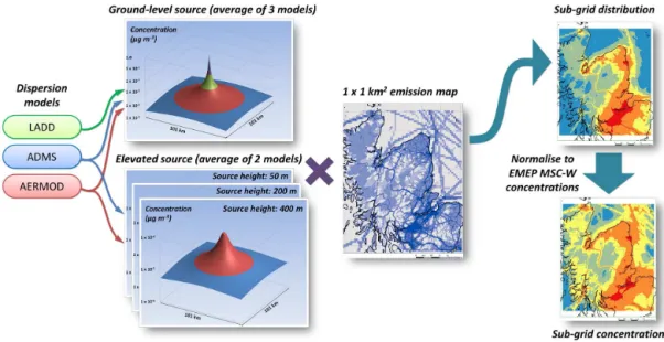
Figure 2.Schematic showing the process of producing the sub-grid concentration predictions from short-range dispersion model simulations and high-spatial-resolution emission data.
3 Model development
The sub-grid 1×1 km2concentration estimates were
calcu-lated from three components: the EMEP 50×50 km2
con-centration predictions, the 1×1 km2 emission data and an
estimate of short-range (<50 km) pollutant dispersion. Fig-ure 2 shows a schematic of the process. Short-range pol-lutant dispersion was parameterised using a simple sce-nario of a single 1×1 km2source with an emission rate of
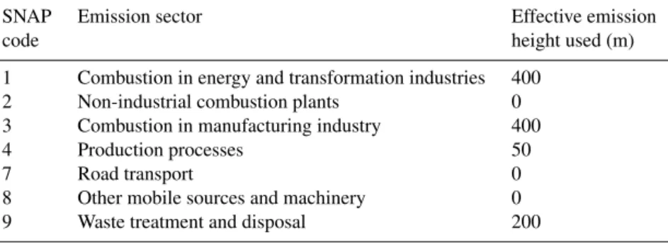
1 Mg km−2yr−1in the centre of a square domain (of dimen-sions 101×101 km2). Although individual sources are gen-erally smaller than this, this value was used to match the spa-tial resolution of the emission data. For NO2, the assump-tion was made that annual mean NO2concentrations are lin-early correlated with those of NOx. This allowed us to use the NOx emissions for the calculation of NO2 concentra-tions without considering photochemical reacconcentra-tions. An anal-ysis of the 2008 mean annual concentrations for the 1478 sites in the Air Quality e-Reporting database (formerly Air-Base) of the European Environment Agency shows that mea-sured NO2 and NOx concentrations are approximately lin-early correlated with a linear correlation coefficient, r2, of 0.93. For the dispersion of NH3, the source was assumed to be at ground level (a suitable approximation for most agricul-tural sources, which account for more than 90 % of emissions in Europe). Emissions of NOx, on the other hand, can occur over a range of emission heights, depending on the source type. Since the emission height will affect the resulting NO2 concentrations at ground level, it needs to be taken into ac-count. This was done by assigning a representative emis-sion height for each emisemis-sion sector (Selected Nomenclature for Air Pollution (SNAP) code) that contributed more than 1 % of the total domain emissions (Table 1). These
emis-sion heights correspond approximately to the mean effec-tive emission heights used in the EMEP model for the sector emissions. In order to test the sensitivity of the AQR model to the emission heights used, additional simulations were car-ried out using emission heights half and double these val-ues. For the ground-level source, all three dispersion models (ADMS, AERMOD and LADD) were used to simulate the annual mean near-ground-level concentrations of NH3 and NO2on a 1 km grid (for the 101×101 km2domain). For the
elevated source scenarios, only ADMS and AERMOD were used to simulate the annual mean concentrations because the LADD model is not suitable for simulating dispersion from elevated sources (Theobald et al., 2012). A height of 1.5 m was used for the near-ground-level concentrations, because this height is commonly used for concentration monitoring and impact assessments (Cape et al., 2009). These short-range dispersion simulations were carried out using the me-teorological data extracted from the WRF simulations at the centre of each EMEP model grid square. No removal pro-cesses (chemical reactions, dry or wet deposition, etc.) were simulated because these processes depend strongly on local conditions (concentrations of other chemical species, meteo-rological conditions, surface characteristics, etc.).
The result of these simulations was nine concentra-tion fields (kernels), three for ground level sources (three models×one source height) and six for elevated sources
(two models×three source heights) for each
Table 1.Emission heights used for each main emission sector.
SNAP Emission sector Effective emission
code height used (m)
1 Combustion in energy and transformation industries 400
2 Non-industrial combustion plants 0
3 Combustion in manufacturing industry 400
4 Production processes 50
7 Road transport 0
8 Other mobile sources and machinery 0
9 Waste treatment and disposal 200
These model-average kernels were then combined with the emission data using a moving window approach to obtain the sub-grid concentration estimate (C):
C (i, j )=
SNAP X
s n X
i′ m X
j′
E i′, j′D′ i−i′, j−j′,
whereiandjare the sub-grid-cell coordinates,sis the emis-sion sector,i′andj′are the emission grid cell coordinates,E is the emission rate of the emission grid cell (Mg km−2yr−1) and D′ an interpolated dispersion kernel (inverse distance squared weighted interpolation of the kernels for the source EMEP grid square and the eight adjacent grid squares). Since the dispersion kernel has a size of 101×101 grid cells, the
values ofi′andj′range fromi−50 andj−50 toi+50 and
j+50, respectively, with the constraint that they lie within
the modelling domain.
The resulting “sub-grid distributions” provide an estimate of the spatial variability of the concentrations at a 1×1 km2
resolution, which were then used to “redistribute” the EMEP predictions within each 50×50 km2grid square. This step is
necessary since AQR does not take into account large-scale processes such as long-range transport or chemical trans-formations of pollutants, processes that are included in the large-scale model (the EMEP model, in this case). The sim-plest way to do this redistribution would be to multiply the sub-grid distributions by the EMEP predictions and then di-vide by the mean value of the sub-grid distribution for each 50×50 km2grid square. This approach conserves the
sub-grid distribution for each 50×50 km2 square and also has
the same mean concentration as the EMEP prediction. How-ever, it also could lead to large discontinuities at the edges of the EMEP grid squares if the ratio between the mean of the sub-grid distribution and the EMEP prediction differ greatly from that of adjacent squares. To avoid this problem, the ra-tio of the EMEP predicra-tions to the mean value of the sub-grid distribution for each 50×50 km2square was interpolated on
a 1×1 km2grid (using a spline interpolation of the values at
the centre of each grid square in ArcGIS 10.2 (Environmen-tal Systems Research Institute, Redlands, CA, USA)). The interpolated field was then multiplied by the sub-grid distri-bution and then the process was repeated over 10 iterations.
In fact only four to five iterations were necessary to give con-centration fields that differed by a maximum of 1 %. A more detailed description of the process is provided in the Supple-ment.
In order to test the sensitivity of the model to the meteoro-logical data, the above process was repeated with the kernels obtained from the dispersion simulations, using the domain-specific meteorological data and with kernels derived from the dispersion simulations using the synthetic meteorologi-cal data (more details provided in the Supplement).
4 Results
4.1 Sub-grid concentration predictions and model evaluation
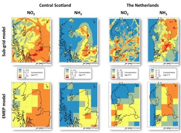
Figure 3 shows the sub-grid concentration predictions for NO2 and NH3 for the two domains (data for the individ-ual domains are provided in Fig. S3.1 in the Supplement). The EMEP concentration fields are also shown for compar-ison. Table 2 shows the evaluation statistics of the EMEP and AQR models for annual mean NO2 concentrations for the Dutch and Scottish monitoring data. In general, AQR is an improvement on the EMEP model alone because the lat-ter generally underestimates concentrations (negative NMB). The mean error of the EMEP model is largest for the Scot-tish dataset with a NMGE of 82 and 70 % for the datasets with and without traffic stations, respectively. The model per-forms worst for the Scottish traffic stations with a mean un-derestimation of 84 %. The EMEP model performs consider-ably better for the Dutch dataset, with 91 % of predictions within a factor of 2 of the observed values, although this drops to 69 % when considering the traffic stations only. The AQR model (using 1×1 km2emissions) also performed best
Figure 3.Sub-grid model predictions (top row) of annual mean concentrations of NO2and NH3for the two domains. EMEP model predic-tions at a resolution of 50×50 km2are shown for comparison (bottom row).
model, AQR performed worst for the Scottish traffic stations, although was a notable improvement over the EMEP model alone. The use of the lower-resolution emissions actually im-proved the performance of AQR for some of the statistics (most notably for the non-traffic stations in the Netherlands domain).
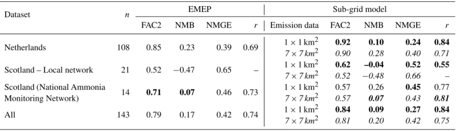
Table 3 shows the evaluation statistics of the EMEP and AQR models for annual mean NH3 concentrations for the Dutch and Scottish monitoring data. In general AQR was an improvement on the EMEP model alone, which performed worse for the local monitoring network, as all monitoring locations were within a single EMEP 50×50 km2 square.
The AQR model (using 1×1 km2emissions) also performed
worst for this dataset, although its performance was still an improvement on that of the EMEP model alone, as it was for all the datasets except for the National Ammonia Monitoring Network sites in Scotland. The use of the 7×7 km2
emis-sions worsened the performance of AQR (with respect to the simulations using the 1×1 km2 emissions) for all datasets
except for the National Ammonia Monitoring Network sites, for which it had a similar performance to the model using the higher-resolution emissions. Figure 4 shows the scatterplots of NO2and NH3concentration predictions of the EMEP and AQR models vs. the observed values for all sites in both do-mains.
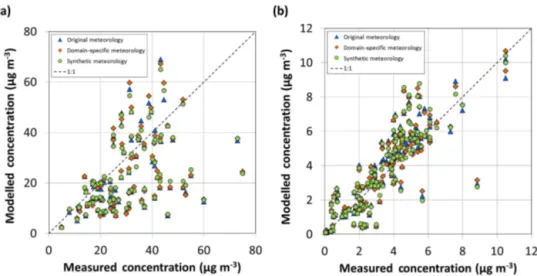
4.2 Sensitivity of sub-grid model predictions to model parameters
The use of alternative meteorological datasets only had a small effect on the concentration estimates of the AQR model (Fig. 5). The use of domain-specific data from a single loca-tion affected the concentraloca-tion predicloca-tions by an average of 6 % for NO2and 5 % for NH3although differences of up to 23 % were found for individual measurement sites. Similarly, the use of the synthetic meteorological data affected concen-trations, on average, by 6 and 5 % for NO2and NH3, respec-tively, with a maximum difference of 28 %. Randomising the wind direction data of the domain-specific datasets gave very similar results to those using the synthetic meteorology dataset, with maximum differences of only 1 % (not shown). This suggests that the meteorological factor that most influ-ences the estimates of the AQR model is the wind direction distribution.
Table 2.Performance evaluation of the EMEP and sub-grid models for annual mean NO2concentrations. The best-performing model for each statistic is highlighted in bold. FAC2 is the fraction of model predictions within a factor of 2 of the observations, NMB is the normalised mean bias, NMGE is the normalised mean gross error andris the Pearson correlation coefficient. Italic font highlights the model performance
for the sub-grid model using the lower-resolution emission data.
Dataset n EMEP model Sub-grid model
FAC2 NMB NMGE r Emission data FAC2 NMB NMGE r
Netherlands (All) 43 0.91 −0.24 0.31 0.54 1×1 km
2 0.98 0.05 0.24 0.83
7×7 km2 1.0 −0.08 0.21 0.79
Netherlands (No traffic stations) 30 1.00 −0.06 0.18 0.73 1×1 km
2 0.97 0.07 0.29 0.86
7×7 km2 1.0 0.01 0.21 0.81
Netherlands (Traffic stations only) 13 0.69 −0.45 0.45 0.17 1×1 km
2 1.0 0.02 0.16 0.48
7×7 km2 1.0 −0.18 0.21 0.32
Scotland (All) 48 0.06 −0.82 0.82 0.16 1×1 km2 0.46 –0.50 0.54 0.43
7×7 km2 0.23 −0.63 0.63 0.51
Scotland (No traffic stations) 11 0.27 −0.70 0.70 0.40 1×1 km
2 0.91 –0.08 0.30 0.80
7×7 km2 0.64 −0.38 0.39 0.85
Scotland (Traffic stations only) 37 0.00 −0.84 0.84 0.05 1×1 km2 0.32 –0.56 0.57 0.48
7×7 km2 0.11 −0.67 0.67 0.51
All 91 0.46 −0.58 0.61 – 1×1 km
2 0.70 –0.27 0.41 0.39
7×7 km2 0.59 −0.40 0.46 0.27
Table 3.Performance evaluation of the EMEP and sub-grid models for annual mean NH3concentrations. The best-performing model for each statistic is highlighted in bold. FAC2 is the fraction of model predictions within a factor of 2 of the observations, NMB is the normalised mean bias, NMGE is the normalised mean gross error andris the Pearson correlation coefficient. Italic font highlights the model performance
for the sub-grid model using the lower-resolution emission data.
Dataset n EMEP Sub-grid model
FAC2 NMB NMGE r Emission data FAC2 NMB NMGE r
Netherlands 108 0.85 0.23 0.39 0.69 1×1 km2 0.92 0.10 0.24 0.84
7×7 km2 0.90 0.28 0.40 0.71
Scotland – Local network 21 0.52 −0.47 0.65 – 1×1 km2 0.62 –0.04 0.52 0.55
7×7 km2 0.52 −0.48 0.66 –
Scotland (National Ammonia 14
0.71 0.07 0.46 0.73 1×1 km2 0.57 0.26 0.45 0.77
Monitoring Network) 7×7 km2 0.57 0.07 0.43 0.81
All 143 0.79 0.17 0.42 0.74 1×1 km2 0.84 0.09 0.27 0.84
7×7 km2 0.81 0.20 0.42 0.75
emission heights, model performance was very similar (not shown).
5 Discussion
5.1 An improvement, but is it enough?
These results show that a simple and robust geostatistical ap-proach can be used to improve the EMEP model predictions of NO2 and NH3annual concentrations. This improvement is not surprising considering the large difference in spatial resolutions (50 km vs. 1 km) and the strong link between short-lived pollutants and the spatial distribution of emis-sions. In fact, it is worth looking at whether this improve-ment is mainly a result of the high-resolution emissions and
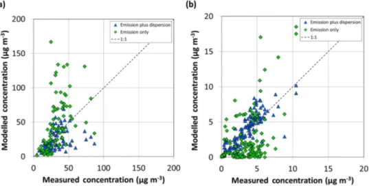
has very little to do with the use of short-range dispersion es-timates. This can be done by repeating the analyses with the 1×1 km2 grid cell emissions as the initial sub-grid
distri-bution. Figure 6 shows that doing this for NO2substantially overestimates concentrations for the mid-range of measured values, whereas for NH3, concentrations are substantially un-derestimated at many sites. The model performance statis-tics for these simulations show that using just the emissions gives lower values of FAC2 (0.60 vs. 0.70 for NO2and 0.28 vs. 0.84 for NH3)and larger bias and error (NMB: 0.36 vs.
Figure 4.Modelled concentrations plotted against measured values for all sites for(a)NO2and(b)NH3. NO2traffic stations are indicated by bold symbol outlines. Plot data provided in the Supplement.
Figure 5.Modelled concentrations plotted against measured values for all sites for(a)NO2and(b)NH3using the original meteorology (as in Fig. 4) and using the domain-specific and synthetic meteorological datasets.
short-range dispersion estimates are necessary for improving on the EMEP model predictions.
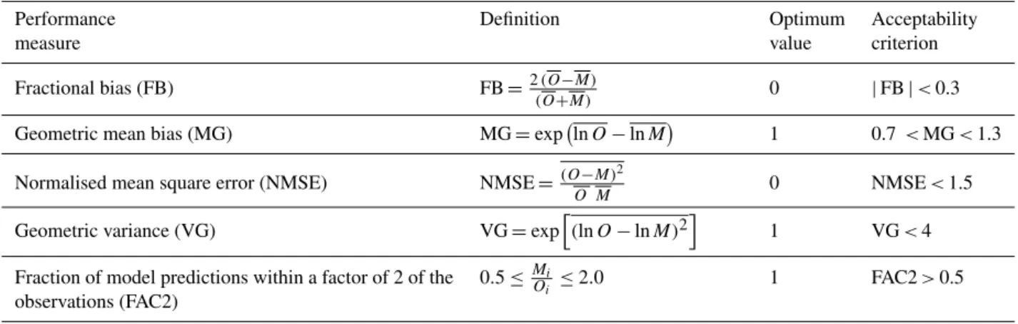
However, is the improvement of AQR over the EMEP model alone large enough to warrant the inclusion of such a sub-grid model into the output processing options of a chemical transport model? In order to answer this question, we can use the concept of model acceptability suggested by Chang and Hanna (2004). This concept can be used to eval-uate whether the EMEP model and/or the AQR model per-form acceptably and, therefore, whether the AQR model rep-resents an improvement on the EMEP model alone, in terms of model acceptability. Hanna and Chang (2012) suggested that an “acceptable” model is one that meets the criteria for more than half of a series of statistical tests. The performance metrics used are fractional bias, geometric mean bias, nor-malised mean square error, geometric variance and FAC2
Figure 6.Modelled concentrations plotted against measured values for all sites for(a)NO2and(b)NH3using the original sub-grid param-eterisation (Emission plus dispersion) and using just the spatial distribution of emissions as the sub-grid distribution (Emission only).
Table 4.Number of model acceptability criteria met for each model and evaluation dataset. Bold font represents acceptable model perfor-mance (≥3 criteria met).
Pollutant Dataset
No. of criteria met
EMEP Sub-grid Sub-grid (1×1 km2 (7×7 km2 emissions) emissions)
NO2
Netherlands All 5 5 5
Netherlands No traffic stations 5 5 5
Netherlands Traffic stations only 3 5 5
Scotland All 0 2 1
Scotland No traffic stations 0 5 3
Scotland Traffic stations only 0 2 0
All 0 3 3
NH3
Netherlands 5 5 5
Scotland Local network 2 5 2
Scotland National Network 5 5 5
All 5 5 5
alone already performs acceptably for this dataset. This can be explained by looking at the number of criteria met for the individual datasets (Table 4). For NO2, The EMEP model performed acceptably for the Netherlands (All) but not for Scotland (All). This is partly due to the Dutch network hav-ing a larger proportion of non-traffic sites (70 % vs. 23 %), which would be more representative of the 50×50 km2grid
cells. However, the EMEP model also performed acceptably for the Dutch traffic stations but neither the EMEP model nor the AQR model performed acceptably for the Scottish traffic stations. Looking more carefully at the traffic stations used in the domains reveals that station siting may have an influence on model performance. According to the information avail-able regarding the Scottish traffic sites, monitoring stations
their monitoring stations far from the influence of individ-ual emission sources in order to be representative of a large area, whereas the local network was located in an area with intensive poultry farming and was designed to assess the in-fluence of individual sources. Since the majority (86 %) of the sites used in the analysis belonged to the national net-works, overall model performance was similar to model per-formance for those networks. The sub-grid approach, there-fore, is most useful where there are large horizontal concen-tration gradients, such as within large cities (for NO2)or ar-eas with intensive agriculture (for NH3), which is where the largest impacts are most likely to occur.
It is also worth briefly comparing the improvements in model performance with those reported by other studies. Denby et al. (2011) showed that the population-weighted concentration for NO2 was, on average, 44 % higher with their sub-grid parameterisation than that calculated using the original concentrations from the EMEP model. Although not directly comparable (since we do not calculate population-weighted concentrations), NO2concentrations estimated us-ing the AQR model are, on average, 77 % higher than those of the EMEP model at the monitoring station locations. De-spite this increase, the AQR estimates are still, on average, 27 % lower than the measured concentrations. Janssen et al. (2012) showed that their approach of downscaling mod-elled concentrations from 15×15 km2to 3×3 km2reduced
model error by about 20 %. The AQR model for NO2reduced model error by 30–40 %, although for a larger change in res-olution (50×50 km2to 1×1 km2). In the study by Schaap et al. (2015), increasing the spatial resolution from approx. 56×56 km2 to 7×7 km2 increased the correlation (r) be-tween the models’ predictions and hourly urban background NO2concentrations from approx. 0.1–0.4 to 0.6–0.7 and re-duced model bias by approx. 60–90 % for most of the mod-els. For a similar change in spatial resolution (50×50 km2
to 7×7 km2), the AQR model for annual mean NO2 concen-trations using the low-resolution emissions increasedrfrom 0.16–0.54 to 0.51–0.85 and reduced model bias by approx. 20–70 %.
5.2 How can the sub-grid approach be applied? Two potential uses of the sub-grid approach can be envis-aged: a Europe-wide application to provide a spatial assess-ment of exceedance of NO2 and NH3 annual limit values or critical levels and the assessment of individual emission hotspots in areas where detailed modelling assessments are not available but high-resolution emission data are. In the latter case, if the hotspot domain is located within a single EMEP 50×50 km2 grid square, the smoothing step would
not be necessary. The Europe-wide application would require high-spatial-resolution emission data for the whole domain. There is, as far as we are aware, currently no European emis-sion inventory with a spatial resolution close to 1×1 km2.
The highest resolutions available are the 7×7 km2emission
inventories produced for various EU projects (Kuenen et al., 2014; EC4MACS, 2012). As shown above, the use of emis-sion data at this resolution still gives an improvement on the concentration predictions and even performs better than the sub-grid model using the higher-resolution emissions, in some cases.
5.3 Advantage, disadvantages, uncertainties and potential improvements
The AQR model can provide more accurate concentration predictions than the EMEP model alone, especially close to emission sources. However, this approach has only been tested for annual mean NO2 and NH3 concentrations, al-though it could potentially be extended to other short-lived pollutants and shorter timescales (daily or hourly). This means that the model cannot currently be used to assess exceedance of short-term limit values (e.g. for Europe, an hourly mean concentration of 200 µg NO2m−3 more than 18 times in one year) although, as shown by Kiesewetter et al. (2013), the annual mean limit values for NO2are the more stringent target. Critical levels for ammonia are expressed as annual mean concentrations and so a sub-grid model with a higher temporal resolution is not necessary. The other limita-tion of the approach is the need for high-resolulimita-tion emission data although, as shown above, the use of emission data with a resolution of 7×7 km2already produces improvements in
model performance compared with the original ACTM con-centration estimates.
The various assumptions and simplifications made in the development of AQR introduce uncertainty in the model es-timates. The omission of NOx photochemistry and the as-sumption that annual mean NO2concentrations are linearly correlated with those of NOx was justified above by the fact that measured concentrations across Europe are approx-imately linearly correlated (r2=0.93). However, a more
disper-sion parameterisations, but wet-deposition has been implic-itly included in ACTM predictions, and timescales for dry deposition are usually far larger than those for sub-grid mix-ing. Again, given the AQR model has a mean error of 41 and 27 % for NO2 and NH3, respectively, the benefits of AQR seem greater than any uncertainty as a result of omitting these processes. Finally, another simplification is the use of a 1×1 km2source for parameterising short-range dispersion.
In reality sources are generally smaller than this and so this simplification may result in incorrect concentration gradients close to small or linear NOxsources (e.g. chimney stacks or motorways). However, on average, transport emissions con-tribute more than 90 % of the estimated concentrations, most of which are in urban areas where a 1×1 km2source is
prob-ably an adequate representation of a dense urban road net-work. In addition, we rarely know the location of stacks in emission inventories to better than 1 km resolution, and usu-ally with no or very limited information on plume rise and height.
With regards to potential improvements, in addition to the extension to shorter time periods, it also should be possible to incorporate stack parameters (effective emission heights and the contribution of stack emissions to the emissions of a par-ticular grid square) from officially reported data and/or other data sources, if these become more readily available. This would potentially improve concentration estimates close to large stack sources. As shown above, model performance is poorer for sites very close to roads and so the inclusion of a roadside increment model could also improve the model esti-mates. However, by increasing the complexity of the model, we have to be careful not to lose sight of the objective of the AQR model, which is to provide a robust and simple method of post-processing concentrations estimated by an ACTM.
The sub-grid approach also has the potential to be ap-plied to other pollutants for which there is a strong rela-tionship between emissions and concentrations. Zhang and Wu (2013) analysed air-quality simulations of the CMAQ model to quantify the influence of a range of processes on the atmospheric concentrations of several pollutants. The species that were most strongly influenced by emission processes were NH3, NO, NO2, SO2, PM2.5, SO2−4 , elemental carbon and primary organic aerosol and are, therefore, potential can-didates for an extension of the model. The spatial distribution of ozone, a secondary pollutant, cannot be estimated based on emissions but its inverse relationship with NOxcould be exploited to model the sub-grid variability. Apart from con-centrations, it may also be possible to develop a sub-grid model for processes such as wet deposition of nitrogen or sul-phur, for which high-resolution rainfall maps could be used to estimate the sub-grid distributions. Dry deposition of re-duced nitrogen could also be modelled using the NH3 con-centration distribution and land-cover parameters, assuming that most of the deposition is in the form of NH3. Dry de-position of oxidised nitrogen would be more difficult since there is no one dominant species that contributes.
6 Conclusions
The sub-grid spatial variability of the annual mean NO2and NH3 concentrations predicted by an atmospheric chemistry and transport model can be estimated by combining the pre-dictions with high-spatial-resolution emission datasets and short-range dispersion fields. This paper describes the de-velopment of the Air Quality Re-gridder (AQR) model and its application to two test domains in Europe. Comparison of annual mean concentrations estimated by AQR with mea-sured values within both domains shows that the AQR model represents an improvement on the predictions of the atmo-spheric chemistry and transport model, reducing both model error and bias and increasing the spatial correlation with the measured concentrations.
7 Code/data availability
The AQR model code (in the R programming language) plus example input and output files for the simulations using syn-thetic meteorological data are provided in the Supplement.
Appendix A: Descriptions of the performance metrics used
Table A1.The four metrics relating modelled concentrations (Mi)with the observed values (Oi), used for evaluating model performance.
Performance measure Definition
Fraction of model predictions within a factor of 2 of the observations (FAC2): 0.5≤Mi Oi ≤2.0
Normalised mean bias: NMB=
n P i=1
Mi−Oi
n P i=1
Oi
Normalised mean gross error: NMGE=
n P i=1
|Mi−Oi|
n P i=1
Oi
Pearson correlation coefficient: r= 1
(n−1) n P
i=1 M
i−M σM
Oi−O σO
Table A2.The five performance measures relating modelled concentrations (Mi) with the observed values (Oi), used to assess model acceptability.
Performance Definition Optimum Acceptability
measure value criterion
Fractional bias (FB) FB=2(O−M)
(O+M) 0 |FB|<0.3
Geometric mean bias (MG) MG=exp lnO−lnM 1 0.7
<MG<1.3
Normalised mean square error (NMSE) NMSE=(O−M)2
O M 0 NMSE<1.5
Geometric variance (VG) VG=exp
h
(lnO−lnM)2 i
1 VG<4
Fraction of model predictions within a factor of 2 of the observations (FAC2)
0.5≤Mi
The Supplement related to this article is available online at doi:10.5194/gmd-9-4475-2016-supplement.
Author contributions. Model development and evaluation was
prin-cipally carried out by M. R. Theobald with contributions on the de-sign of the sub-grid modelling methodology from D. Simpson and M. Vieno. Emission datasets were prepared by M. Vieno and the manuscript was prepared by M. Theobald with contributions from both co-authors.
Acknowledgements. The work presented in this paper was funded
through the EU projects: NitroEurope IP (Project No.: 017841) and ECLAIRE (project no.: 282910), and EMEP under UNECE. We would like to thank Sim Tang at CEH Edinburgh for providing the NAMN data from the Defra project AQ0647 UK Eutrophying and Acidifying Atmospheric Pollutants (UKEAP), Mhairi Coyle at CEH Edinburgh for providing the Easter Bush meteorological data, the Cabauw Experimental Site for Atmospheric Research (Cesar) database for the Cabauw meteorological data, Roy Wichink Kruit at RIVM for the Dutch NO2concentration data and Dorien Lolkema at RIVM for the Dutch NH3concentration data.
Edited by: A. Colette
Reviewed by: two anonymous referees
References
Aggarwal, P. and Jain, S.: Impact of air pollutants from surface transport sources on human health: A modeling and epidemio-logical approach, Environ. Int., 83, 146–157, 2015.
Amann, M., Bertok, I., Borken-Kleefeld, J., Cofala, J., Heyes, C., Höglund-Isaksson, L., Klimont, Z., Nguyen, B., Posch, M., and Rafaj, P.: Cost-effective control of air quality and greenhouse gases in Europe: Modeling and policy applications, Environ. Modell. Softw., 26, 1489–1501, 2011.
Bessagnet, B., Hodzic, A., Vautard, R., Beekmann, M., Cheinet, S., Honoré, C., Liousse, C., and Rouil, L.: Aerosol modeling with CHIMERE – preliminary evaluation at the continental scale, At-mos. Environ., 38, 2803–2817, 2004.
Cape, J. N., van der Eerden, L. J., Sheppard, L. J., Leith, I. D., and Sutton, M. A.: Evidence for changing the critical level for am-monia, Environ. Pollut., 157, 1033–1037, 2009.
Carruthers, D. J., Holroyd, R. J., Hunt, J. C. R., Weng, W. S., Robins, A. G., Apsley, D. D., Thompson, D. J., and Smith, F. B.: UK-ADMS: A new approach to modelling dispersion in the earth’s atmospheric boundary layer, J. Wind. Eng. Ind. Aerod., 52, 139–153, 1994.
Carslaw, D. C. and Ropkins, K.: Openair – an R package for air quality data analysis, Environ. Modell. Softw., 27, 52–61, 2012. Chang, J. C. and Hanna, S. R.: Air quality model performance
eval-uation, Meteorol. Atmos. Phys., 87, 167–196, 2004.
Ching, J., Isakov, V., Majeed, M., and Irwin, J.: An approach for in-corporating sub-grid variability information into air quality mod-elling, Proceedings of the 14th Joint Conference on the Appli-cations of Air Pollution Meteorology with the Air and Waste
Management Association, Atlanta, USA, 27 January–3 February 2006.
Cimorelli, A. J., Perry, S. G., Venkatram, A., Weil, J. C., Paine, R. J., Wilson, R. B., Lee, R. F., Peters, W. D., Brode, R. W., and Pauimer, J. O.: AERMOD: Description of Model Formulation Version 02222. United States Environmental Protection Agency, Research Triangle Park, NC 27711, USA, 85 pp., 2002. CLRTAP, Chapter 2 of the Draft Manual on Methodologies
and Criteria for Modelling and Mapping Critical Loads & Levels and Air Pollution Effects, Risks and Trends, available at: http://www.rivm.nl/media/documenten/cce/manual/ Ch2-MapMan-2014-08.pdf (last access: 12 December 2016), 2014.
Cuvelier, C., Thunis, P., Karam, D., Schaap, M., Hendriks, C., Kra-nenburg, R., Fagerli, H., Nyiri, A., Simpson, D., Wind, P., Schulz, M., Bessagnet, B., Colette, A., Terrenoire, E., Rouïl, L., Stern, R., Graff, A., Baldasano, J. M., and Pay, M. T.: ScaleDep: per-formance of European chemistry-transport models as function of horizontal special resolution, EMEP Technical report 1/2013, 63 pp., 2013.
Denby, B., Cassiani, M., de Smet, P., de Leeuw, F., and Horálek, J.: Sub-grid variability and its impact on European wide air quality exposure assessment, Atmos. Environ., 45, 4220–4229, 2011. Dentener, F., Drevet, J., Lamarque, J. F., Bey, I., Eickhout, B.,
Fiore, A. M., Hauglustaine, D., Horowitz, L.W., Krol, M., Kul-shrestha, U. C., Lawrence, M., Galy-Lacaux, C., Rast, S., Shin-dell, D., Stevenson, D., Van Noije, T., Atherton, C., Bell, N., Bergman, D., Butler, T., Cofala, J., Collins, B., Doherty, R., Ellingsen, K., Galloway, J., Gauss, M., Montanaro, V., Müller, J. F., Pitari, G., Rodriguez, J., Sanderson, M., Solmon, F., Stra-han, S., Schultz, M., Sudo, K., Szopa, S., and Wild, O.: Ni-trogen and sulfur deposition on regional and global scales: a multimodel evaluation, Global Biogeochem. Cy., 20, GB4003, doi:10.1029/2005GB002672, 2006.
de Smet, P., de Leeuw, F., Horálek, J., and Kurfürst, P.: A European compilation of national air quality maps based on modelling, ETC/ACM Technical Paper 2013/3, March 2013.
Dragosits, U., Theobald, M. R., Place, C. J., Lord, E., Webb, J., Hill, J., ApSimon, H. M., and Sutton, M. A.: Ammonia emission, de-position and impact assessment at the field scale: a case study of sub-grid spatial variability, Environ. Pollut., 117, 147–158, 2002. EC4MACS.: The GAINS Integrated Assessment Model, EC4MACS Report, available at: http://www.ec4macs.eu/ content/report/EC4MACS_Publications/MR_Finalinpdf/ GAINS_Methodologies_Final.pdf (last access: 12 Decem-ber 2016), 2012.
EMEP: Transboundary particulate matter, photo-oxidants, acidify-ing and eutrophyacidify-ing components, Status Report 1/2015, EMEP MSC-W, The Norwegian Meteorological Institute, Oslo, Nor-way, 2015.
Fagerli, H. and Aas, W.: Trends of nitrogen in air and precipitation: Model results and observations at EMEP sites in Europe, 1980– 2003, Environ. Pollut., 154, 448–461, 2008.
Galvis, B., Bergin, M., Boylan, J., Huang, Y., Bergin, M., and Rus-sell, A. G.: Air quality impacts and health-benefit valuation of a low-emission technology for rail yard locomotives in Atlanta Georgia, Sci. Total Environ., 533, 156–164, 2015.
ISC Dispersion Models for Regulatory Applications, Report No. P362. Environment Agency, Bristol, UK, 2000.
Hallsworth, S., Dore, A., Bealey, W., Dragosits, U., Vieno, M., Hell-sten, S., Tang, Y., and Sutton, M.: The role of indicator choice in quantifying the threat of atmospheric ammonia to the “Natura 2000”network, Environ. Sci. Policy, 13, 671–687, 2010. Hanna, S. R. and Chang, J.: Setting Acceptance Criteria for Air
Quality Models, Air Pollution Modeling and its Application XXI, 479–484, 2012.
Isakov, V., Irwin, J. S. and Ching, J.: Using CMAQ for exposure modeling and characterizing the subgrid variability for exposure estimates, J. Appl. Meteorol. Clim., 46, 1354–1371, 2007. Janssen, S. and Thunis, P.: Fairmode’s composite mapping
exer-cise, Proceedings of the 10th International Conference on Air Quality – Science and Application, Milan, Italy, 14–18 March 2016, available at: http://www.airqualityconference.org/, last ac-cess: 12 December 2016.
Janssen, S., Dumont, G., Fierens, F., Deutsch, F., Maiheu, B., Celis, D., Trimpeneers, E., and Mensink, C.: Land use to characterize spatial representativeness of air quality monitoring stations and its relevance for model validation, Atmos. Environ., 59, 492–500, 2012.
Kiesewetter, G., Borken-Kleefeld, J., Heyes, C., Bertok, I., Schoepp, W., Thunis, P., Bessagnet, B., Terrenoire, E., and Amann, M.: Modelling compliance with NO2and PM10air qual-ity limit values in the GAINS model. TSAP Report no. 9, IIASA., 2013.
Kiesewetter, G., Borken-Kleefeld, J., Schöpp, W., Heyes, C., Thu-nis, P., Bessagnet, B., Terrenoire, E., Gsella, A., and Amann, M.: Modelling NO2concentrations at the street level in the GAINS integrated assessment model: projections under current legis-lation, Atmos. Chem. Phys., 14, 813–829, doi:10.5194/acp-14-813-2014, 2014.
Kuenen, J. J. P., Visschedijk, A. J. H., Jozwicka, M., and Denier van der Gon, H. A. C.: TNO-MACC_II emission inventory; a multi-year (2003–2009) consistent high-resolution European emission inventory for air quality modelling, Atmos. Chem. Phys., 14, 10963–10976, doi:10.5194/acp-14-10963-2014, 2014.
Lolkema, D. E., Noordijk, H., Stolk, A. P., Hoogerbrugge, R., van Zanten, M. C., and van Pul, W. A. J.: The Measuring Ammonia in Nature (MAN) network in the Netherlands, Biogeosciences, 12, 5133–5142, doi:10.5194/bg-12-5133-2015, 2015.
Nguyen, P., Stefess, G., de Jonge, D., Snijder, A., Hermans, P., van Loon, S., and Hoogerbrugge, R.: Evaluation of the repre-sentativeness of the Dutch air quality monitoring stations: The national, Amsterdam, Noord-Holland, Rijnmond-area, Limburg and Noord-Brabant networks, RIVM report 680704021, 2013. Oxley, T. and ApSimon, H.: Space, time and nesting integrated
as-sessment models, Environ. Modell. Softw., 22, 1732–1749, 2007. Schaap, M., Cuvelier, C., Hendriks, C., Bessagnet, B., Baldasano, J. M., Colette, A., Thunis, P., Karam, D., Fagerli, H., Graff, A., Kra-nenburg, R., Nyiri, A., Pay, M. T., Rouil, L., Schulz, M., Simp-son, D., Stern, R., Terrenoire, E., and Wind, P.: Performance of European chemistry transport models as function of horizontal resolution, Atmos. Environ., 112, 90–105, 2015.
Simpson, D., Butterbach-Bahl, K., Fagerli, H., Kesik, M., Skiba, U., and Tang, S.: Deposition and emissions of reactive nitrogen over European forests: a modelling study, Atmos. Environ., 40, 5712–5726, 2006.
Simpson, D., Benedictow, A., Berge, H., Bergström, R., Emberson, L. D., Fagerli, H., Flechard, C. R., Hayman, G. D., Gauss, M., Jonson, J. E., Jenkin, M. E., Nyíri, A., Richter, C., Semeena, V. S., Tsyro, S., Tuovinen, J.-P., Valdebenito, Á., and Wind, P.: The EMEP MSC-W chemical transport model – technical descrip-tion, Atmos. Chem. Phys., 12, 7825–7865, doi:10.5194/acp-12-7825-2012, 2012.
Spanton, A. M., Hall, D. J., Dunkerley, F., Griffiths, R. F., and Bennett, M.: A Dispersion Model Intercomparison Archive. Pro-ceedings of 9th Int. Conf. on Harmonisation within Atmospheric Dispersion Modelling for Regulatory Purposes, Garmisch-Partenkirchen, Germany, 1–4 June 2004.
Sutton, M. A., Tang, Y. S., Dragosits, U., Fournier, N., Dore, A. J., Smith, R. I., Weston, K. J., and Fowler, D.: A spatial analysis of atmospheric ammonia and ammonium in the UK, The Scientific World Journal, 1 Suppl 2, 275–286, 2001.
Theobald, M. R., Løfstrøm, P., Walker, J., Andersen, H. V., Peder-sen, P., Vallejo, A., and Sutton, M. A.: An intercomparison of models used to simulate the short-range atmospheric dispersion of agricultural ammonia emissions, Environ. Modell. Softw., 37, 90–102, 2012.
Vieno, M., Dore, A. J., Stevenson, D. S., Doherty, R., Heal, M. R., Reis, S., Hallsworth, S., Tarrason, L., Wind, P., Fowler, D., Simp-son, D., and Sutton, M. A.: Modelling surface ozone during the 2003 heat-wave in the UK, Atmos. Chem. Phys., 10, 7963–7978, doi:10.5194/acp-10-7963-2010, 2010.
Vieno, M., Heal, M. R., Hallsworth, S., Famulari, D., Doherty, R. M., Dore, A. J., Tang, Y. S., Braban, C. F., Leaver, D., Sutton, M. A., and Reis, S.: The role of long-range transport and domes-tic emissions in determining atmospheric secondary inorganic particle concentrations across the UK, Atmos. Chem. Phys., 14, 8435–8447, doi:10.5194/acp-14-8435-2014, 2014.
Vogt, E., Dragosits, U., Braban, C. F., Theobald, M. R., Dore, A. J., van Dijk, N., Tang, Y. S., McDonald, C., Murray, S., Rees, R. M., and Sutton, M. A.: Heterogeneity of atmospheric ammonia at the landscape scale and consequences for environmental impact assessment, Environ. Pollut., 179, 120–131, 2013.
von Bobrutzki, K., Braban, C. F., Famulari, D., Jones, S. K., Black-all, T., Smith, T. E. L., Blom, M., Coe, H., Gallagher, M., Gha-laieny, M., McGillen, M. R., Percival, C. J., Whitehead, J. D., El-lis, R., Murphy, J., Mohacsi, A., Pogany, A., Junninen, H., Ranta-nen, S., Sutton, M. A., and Nemitz, E.: Field inter-comparison of eleven atmospheric ammonia measurement techniques, Atmos. Meas. Tech., 3, 91–112, doi:10.5194/amt-3-91-2010, 2010. Zhang, Y. and Wu, S.: Understanding of the Fate of Atmospheric