Pattern Recognition-Based Environment
Identification for Robust Wireless Devices
Positioning
Nesreen I. Ziedan
Computer and Systems Engineering Department Faculty of Engineering, Zagazig University
Zagazig, Egypt
Abstract—There has been a continuous increase in the demands for Global Navigation Satellite System (GNSS) receivers in a wide range of applications. More and more wireless and mobile devices are equipped with built-in GNSS receivers; their users’ mobility behavior can result in challenging signal conditions that have detrimental effects on the receivers’ tracking and positioning accuracy. A major error source is the multipath signals, which are signals that are reflected off different surfaces and propagated to the receiver's antenna via different paths. Analysis of the received multipath signals indicated that their characteristics depend on the surrounding environment. This paper introduces a machine-learning pattern recognition algorithm that utilizes the aforementioned dependency to classify the multipath signals’ characteristics and identify the surrounding environment. The identified environment is utilized in a novel adaptive tracking technique that enables a GNSS receiver to change its tracking strategy to best suit the current signal condition. This will lead to a robust positioning under challenging signal conditions. The algorithm is verified using real and simulated Global Positioning System (GPS) signals with accurate multipath models.
Keywords-component; GPS; GNSS; machine learning; pattern recognition; PCA; PNN; multipath.
I. INTRODUCTION
A Global Navigation Satellite System (GNSS) [1, 2] is a radio navigation system that employs spread spectrum techniques to transmit ranging signals and navigation data. The ranging signals are used by a GNSS receiver to identify the visible GNSS satellites and measure the distance between the visible GNSS satellites and the GNSS receiver. The measured distances are used with the navigation data to solve the navigation equation to determine the user’s 3-diemntional position and velocity. Examples of GNSS systems are the US Global Positioning System (GPS), the Russian GLONASS, and the European Galileo Navigation System.
GNSS receivers perform three main functions: signal acquisition, signal tracking, and navigation message decoding. Signal acquisition identifies the visible satellites and provides rough estimates of the Doppler frequency, fd, and the ranging
code delay, . Signal tracking applies closed loop tracking techniques to provide continuous accurate estimates of the carrier phase, the Doppler frequency, the Doppler rate, and the
code delay. Those estimates are used to measure the distance between the GNSS satellite and the receiver.
GNSS receivers can give positioning accuracy up to a few millimeters when the receiver is stable and has a clear view of the sky, where the Line-of-Sight (LOS) signal is received with strong power. However, in environments like urban, suburban, and indoor, the received signals suffer from attenuation and multipath errors because of the surrounding objects [3]. In
addition, the user’s mobility behavior can subject the receiver
to changing and unstable signals dynamics. This leads to deterioration in the tracking and positioning accuracy.
Multipath signals are a major error source. They appear when the GNSS satellite signals are reflected off different surfaces and propagated to the receiver's antenna via different paths. This leads to the reception of several versions of the same signal, which causes tracking errors. Analysis of the received signals indicated that their characteristics depend on the surrounding environment [4, 5, 6, 7, 8]. Urban, sub-urban and indoor environments generate different characteristics, which include multipath signals' parameters like the number and duration of echoes and signals power, and LOS signal's parameters like amplitude fluctuation, Doppler shift and rate. Different tracking strategies are needed for each environment to mitigate multipath errors and maximize the tracking performance.
There have been numerous tracking strategies that are optimized for specific signal condition or environment. For example, conventional tracking techniques [1, 2] are used with strong signals. Kalman Filter based techniques are used with weak signals [3, 9]. Tightly-coupled GNSS with Inertial Navigation System (INS) techniques are used with weak interrupted signals or blocked signals [10]. Open-loop batch processing, and combined batch and sequential processing techniques are used in high dynamic applications [11]. Particle Filter-based techniques are used for tracking in multipath environments [12, 13, 14].
of a tacking strategy selector that adaptively changes the tracking strategy to best suit the current signal condition.
The LτS and multipath signals’ patterns of each possible environment are represented by a class. The introduced algorithm is structured into several channels, each of which is tuned to one of the classes. The channels are trained on sets of patterns from each class, and then they are used to classify new unclassified patterns. The proposed pattern recognition algorithm performs two main functions, which are feature extraction and pattern classification. Feature extraction is the process of learning the distinctive characteristics of the data and removing redundant data. This is done to get a compact and robust representation of the distinctive features of each class, thus reducing the processing overhead and memory requirements without degrading the classification performance. Feature extraction, which is used in image and face recognition [15, 16, 17, 18, 19, 20, 21, 22, 23], is performed using a Principal Component Analysis (PCA) approach. Pattern classification is the process of building neurons that capture the dominant features shared by different realizations of each class, and then classifying new patterns into one of the classes. Neurons are computational units that are connected by weighted links. Pattern classification has many applications, like radar detection and remote sensing [24, 25, 26]; it is performed here using a multi-layer feedforward Probabilistic Neural Network (PNN) approach [27, 28, 29, 30, 31,32].
The proposed tracking strategy selector module utilizes both closed loop tracking techniques and open loop tracking techniques to accommodate various patterns. Open loop tracking techniques are activated in unstable or rapidly changing signal conditions, while closed loop tracking techniques are activated in relatively stable or light multipath environments. In addition, based on the environment classification, the activated technique adjusts its parameters to achieve reliable tracking performance.
The rest of this paper is organized as follows. Section II presents some signals patterns that appear in urban and suburban environments. Section III presents the proposed pattern recognition algorithm. Section IV discusses the adaptive tracking concept. Section V presents some testing and results to verify the algorithm performance. Section VI concludes the paper.
II.LOSAND MULTIPATH PATTERNS
The received GNSS signal consists of the LOS signal and NMP multipath signals. The down-converted sampled received GPS C/A signal can be expressed as
Where, A is the signal amplitude. d is the navigation data. C is the ranging code. fIF is the intermediate frequency (IF). fd
is the Doppler shift. α is the Doppler rate. θn is the phase. is the code delay. n is the measurement noise. m is the attenuation in the multipath signal amplitude relative to the
LOS signal amplitude. m is the multipath signal delay. Φm is the multipath phase advance relative to the LOS signal.
The received signal is processed by the receiver to generate the integrated signal, which has the form
Where, Λ is a reference amplitude that is used to express any amplitude relative to it, e.g. the LOS amplitude is A = γ0 Λ.
γm = γ0 m. R(.) is the auto-correlation function. eu is the code delay estimation error at time instance u. feu is the Doppler shift estimation error. θeu is the phase estimation error. Δ is a code delay relative to the estimated code delay of the LOS signal. Ti is the integration time.
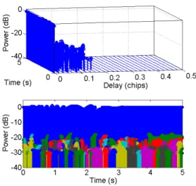
The attenuation of the LOS signal and the number and distribution of the multipath signals depend on the surrounding environment. Elaborate studies exploring the effects of urban and suburban environments on real signals were presented in [4, 5, 6, 7, 8]. Identifying the distribution of the LOS and multipath signals will enable adjusting the tracking strategy or the tracking parameters to obtain the best attainable tracking performance under various signal conditions. The software provided in [33] is used to generate received signal patterns that typically appear in urban and suburban environments. Some of these patterns are shown in Figs. 1-3. Each figure shows two plots: a 3-dimensional (3-D) plot that expresses the pattern in time, delay, and power; and a 2-D plot that is a rotated version of the 3-D plot.
Fig. 1 shows a pattern generated in a suburban environment when a user is walking at a speed of 4 miles/hour. The pattern exhibits a strong LOS signal with light multipath signals that have weak power compared to the LOS signal. Fig. 2 shows a pattern generated in a suburban environment when a car is moving at a speed of 20 miles/hour. The LOS signal here is weaker than the LOS signal shown in Fig. 1, and the multipath signals are not much weaker than the LOS signal. The pattern exhibits changing characteristics over 5 seconds, and it can be divided into several sub-patterns. For example, from 0-2 seconds the LOS signal is stronger than the multipath signals, around 2 seconds the LOS signal appears to be completely blocked, from 2-3.5 seconds the LOS signal is weaker than the multipath signals, and around 3.5 seconds there are no multipath signals. Fig. 3 shows a pattern generated in an urban environment when a car is moving at a speed of 20 miles/hour. This pattern also exhibits changing characteristics. The LOS signal either suffers from complete blockage, or frequent interruption over a short period of time. The multipath signals in this urban environment are denser than the suburban cases.
The distribution of the surrounding objects and their shape and height directly contribute to the multipath signals (echoes) distribution. Indoor patterns are usually characterized by weak or blocked LOS signals. Obviously, different patterns will need different tracking strategies to achieve optimized tracking performance, and hence optimized positioning accuracy. (1)
Figure 1. Multipath pattern in a pedestrian suburban environment.
Figure 2. Multipath pattern in a car suburban environment.
Figure 3. Multipath pattern in a car urban environment.
III. MULTIPATH PATTERN RECOGNITION (MPR)
3-D patterns can be constructed from different parameters, like amplitude and phase. Each 3-D pattern is represented by a
2-D matrix, where each entry contains the value of a parameter at a code delay and a time instance. For example, a matrix that expresses the amplitude pattern over Np code delays and NPNN time instances is
A PNN maps an input feature vector to an output class. The feature vector describes the similarities and differences between the features of the pattern in question and the dominant features of the training patterns. The process of learning the dominant features of the training patterns, and removing redundant data, is feature extraction.
Feature extraction is performed using PCA. In PCA, an eigen-decomposition is performed on the covariance matrix of the training patterns. The eigenvalues are sorted in a decreasing order, and then the eigenvectors that are associated with the largest eigenvalues, i.e. the dominant eigenvectors, are retained. A reduced-size pattern matrix is reconstructed with the dominant eigenvectors. The training patterns are divided into Ncl classes, where the characteristics of each class are selected based on the desired identification criteria. The criteria can be chosen to characterize the reflected signals (e.g. dense reflected signals, occasionally blocked LOS signal), a specific surrounding objects (e.g. trees, buildings), or a specific environment (e.g. urban, suburban). The classes should have distinctive characteristics relative to each other. The criteria and the number of steps, NPNN, can be adjusted and optimized to fit the classification objective. The following will use the
pattern matrix γ to explain the proposed algorithm.
Assume that there are a total of Ntr training patterns from all the Ncl classes. The PCA decomposition on the training
matrices γk where k = 1, …, σtr, is done as follows:
Each γk matrix is converted into one vector, by reading the matrix column by column.
The Ntr vectors are joined in one matrix, where each row contains one vector. So, a matrix of size Ntr (Np NPNN) is obtained; define it as Ώγ.
The mean pattern is calculated. This is the mean of each column of Ώγ. A row vector, γm, of size (Np NPNN) is obtained. The mean pattern is subtracted from each row in Ώγto get a matrix defined as ξγ.
eigenvalues), and not all the (Np NPNN) eigenvectors. Getting the eigen patterns is done as follows:
An alternative covariance matrix of size Ntr . Ntr is found as tr = ξγ ξγH.
The eigenvectors and eigenvalues of the covariance matrix tr are calculated. The eigenvectors are a set of orthonormal vectors.
The eigenvectors are sorted based on the associated eigenvalues. The NEtr dominant eigenvectors are chosen, where NEtr≤ Ntr. The chosen eigenvectors are appended to one matrix, defined as Ґtr, which will have a size of Ntr NEtr.
The eigen patterns are obtain as λtr = ξγ H Ґ
tr, where, λtr has a size of (Np NPNN) . NEtr. Those eigen patterns are orthonormal vectors, and they span NEtr-dimensional subspace, instead of the original (Np NPNN) space. The contribution of each eigen pattern in representing each training pattern is calculated by projecting the training patterns into the pattern space. This results in the following PCA weights: Wtr = λtrHξγH. Where, Wtr has a size of NEtr . Ntr. Each column represents the projection of one training pattern into the pattern space, and each entry in a column represents the contribution of each eigen pattern in expressing the associated training pattern.
This process accomplishes two goals: expressing the patterns in terms of the dominant eigenvectors, i.e. the features that distinctly characterize the patterns; and, reducing the size of the training patterns.
The concept of classification of a new unclassified pattern is to find the class that best describes that pattern. The classification is based on finding the class with the minimum Euclidean distance to the projection of the new pattern. To classify a new pattern, γn, it is first projected into the training
pattern space as follows:
1) γn is converted into one vector, by reading the matrix column by column. A vector γ n is obtained.
2) The mean pattern, γm, is subtracted from γ n to get a vector γn.
3) γn is projected into the training pattern space (i.e. the PCA weights are calculated) as Wp= λtr
H
( γn)H. Where. Wp has a size of NEtr . Ntr.
4) The feature vector of the new pattern can be obtained as
γp = λtr Wp.
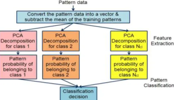
The classification is done using PNN. The introduced PNN is a fully connected network that consists of four layers: input layer, pattern layer, summation layer, and output layer. Fig. 4 illustrates the PNN layers and their connections. The input layer has a number of units equal to the number of variables used in the classification process.
The training patterns are stored in the pattern layer, and they are used to construct the probability density function of each class. The summation layer employs a Bayesian approach to calculate the probability that a new unclassified pattern belongs to each class.
The output layer uses a competitive transfer function to choose the maximum probability and generate an output that indicates the class that the new pattern belongs to it. The introduced MPR algorithm is designed with a flexibility to learn new patterns, and adapt the performance based on new training data. Adding new patterns requires recalculating the weights Wtr.
The number of training patterns available for each class is defined as Nc, where c = 1,…, Ncl. The eigen patterns for each class are defined as λtric, where c is the class index, and i = 1,
…, σc. The PDF for each class is estimated using the Parzen's estimator [24] as follows
Where, L is the λtr vector length, and c is a smoothing factor.
The PCA weight matrix, Wtr, is divided into Ncl matrices, where each matrix contains the weights of one class. Define those matrices as Wtrc, where c is the class index. Each matrix has a size of NEtr.Nc. Define each column vector of Wtrc as Wtri
c
, where i = 1, …, σc. Another PDF, for each class, can be estimated as
Similarly, the PCA weights matrix relating the unclassified pattern to each class, Wp, is divided into Ncl matrices, defined as Wpc, where c is the class index, and p is the new pattern to be classified. Each column vector is defined as Wpic, where, i =
1, …, σc. The summation layer of the PNN calculates the probability that the unclassified pattern belongs to each class. This is done as follows. The distance between each training pattern in each class and the unclassified pattern is found as
The probability that the unclassified pattern belongs to a class c is calculated as
Where, c = 1, … , σcl. The output layer of the PNN uses a decision function based on gpc to classify the unclassified pattern. Fig. 5 outlines the steps of pattern recognition.
Figure 4. Illustration of the PNN layers and their connections.
(3)
(4)
(5)
Figure 5. Illustration of the steps of pattern recognition.
More than one pattern maybe needed to identify the surrounding environment. This is because similar patterns can be generated from different environments, and also some environments can generate several distinctive patterns at different times. The pattern recognition algorithm is modified to avoid misclassification of the environment. Each environment has its own class, and each class consists of Nsc subclasses, where each subclass defines patterns with distinctive features. Training patterns are collected for each subclass. In the classification step, instead of collecting one pattern to identify the environment, Npe patterns are collected over separate times. Each pattern is classified separately, and then the class that most of the patterns are classified to it is chosen, and its corresponding environment is identified as the current surrounding environment. Fig. 6 outlines this approach of environment classification. Another approach to identify the environment is to collect statistics from the unclassified patterns and include them in the classification process. On average, an urban environment has higher number of reflected signals than a suburban environment, and indoor signals are weaker and can incur longer blockage times.
Figure 6. Illustration of the steps of environment recognition.
IV. ADAPTIVE TRACKING STRATEGY SELECTION
Signal acquisition can be done under strong and weak signal conditions, and in low and high dynamics environment [3]. Following a signal acquisition, the receiver obtains rough estimates of the code delay, the Doppler shift, and the Doppler rate. A closed-loop tracking is initialized using the acquisition output, and then it works to refine the parameters estimates and continuously track changes in the code and carrier parameters. Closed-loop tracking techniques are based on generating error
signals proportional to the current errors in the estimated parameters. Those error signals are fed back to the tracking algorithm to readjust the estimated parameters and maintain locks on the code and carrier parameters. A sudden large error in the estimated parameters due to sudden changes in the signal dynamics or the signal condition can cause loss of lock on the signal, and the tracking can no longer continue its operation. In this case, an acquisition process has to be re-initiated to reacquire the signal. If the signal is in an unstable environment, like continuous changes in dynamics, frequent signal blocking, or dense multipath environment, then closed-loop tracking will not be able to achieve lock on the signal. An open-loop tracking can provide the solution to tracking in such cases.
Open-loop tracking performs an acquisition-like process on the received signal, but with a smaller search range in the code delay and Doppler shift. The search range is adjusted based on the signal dynamics and condition. For example, in dense multipath reflected signals, high dynamics will require larger search range than low dynamics.
The output of the introduced MPR algorithm is fed to a tracking strategy selector, which uses the output to decide on a tracking strategy and tune the filters parameters to best suit the signal condition. The tracking algorithms previously introduced for weak signals [3], weak interrupted signals [10], and multipath tracking [14] are used as basis for closed loop tracking. The acquisition algorithms previously introduced for weak signals and high dynamics in [3] are used as basis for open loop tracking. An extra module is added to each algorithm to detect changes in the environment by detecting changes in the carrier to noise ratio C/N0, the signal dynamics, the number of detected multipath signals, or loss of lock. Detecting changes in the signal conditions will invoke a rerun of the MPR algorithm to identify the new signal pattern and/or the environment.
V. TESTING AND RESULTS
Real and simulated GPS C/A signals are used to assess the performance of the algorithm. Urban and suburban multipath patterns are generated using the models in [4, 5, 6, 7, 8] and the software in [33], while indoor and outdoor patterns are simulated. The real GPS data were provided by the University of New South Wales, Australia. The real GPS data had strong LOS signal and no multipath signals. It is processed to add few multipath non-varying signals, and then it is used to generate some of the training patterns for strong outdoor signals. Hardware and software simulators are used as sources for the simulated GPS signals. The hardware simulator’s GPS data were provided by the PLAN group at the University of Calgary, Canada. The software simulator’s GPS data are generated as in [3, 14]. The simulated GPS signals are used with the multipath patterns to get a variety of signals conditions to be used in the verification process.
chosen to accommodate various tracking strategies. Six classes are selected for the test. The classes are as follows:
1) SL-CM: Slow varying LOS signal power with very few non-varying multipath reflected signals.
2) SL-DM: Slow varying LOS signal power with very dense multipath reflected signals.
3) FL-VM: Fast changing LOS signal power with various scenarios for multipath reflected signals.
4) BL-VM: LOS signal with occasional blockage, and with various scenarios for multipath reflected signals.
5) BL-DM: Blocked or very weak LOS signal with dense multipath reflected signals.
6) BL-LM: Blocked or very weak LOS signal with few multipath reflected signals.
A total of 150 training patterns are generated. The integration time, Ti, used here is 5 milliseconds, and each pattern spans 1 second. The patterns are divided into the six aforementioned classes, where each pattern is allocated to the most appropriate class. To test the classification performance, 25 new patterns are generated, where none of them were used in the training process. The probability that each unclassified pattern, p, belongs to one of the classes is calculated as in (6). Those probabilities are normalized as follows:
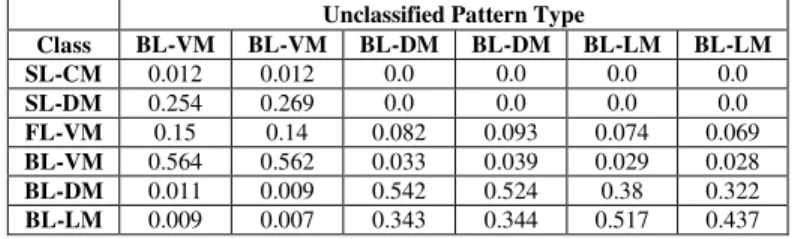
Tables I and II show 11 of the classifications results. Each column contains the result for one unclassified pattern, and each row contains the results for each class type. The pattern with the slow varying LOS signal with non-varying few multipath signals was classified with probability 1 to its class, SL-CM, which means it did not show any similarities to any of the other classes. The number and density of multipath reflected signals can vary from very light to very dense, and there is no actual boundary to classify any possible multipath density pattern into only two classes, However, the classification results indicate how light or how dense a pattern is. This is clear in the results in the last four columns of table II. This indicates that the probability of each class can be used to draw further conclusions about a pattern.
Environment identification test is also conducted. Four environments are defined: Outdoor, indoor, urban, and suburban. The outdoor is defined here as an environment that has very few surrounding objects. Urban and suburban environments structures differ from one place to another. In this test, a suburban environment is a one with wide streets, trees, and low-rise buildings with large separation between them. Urban environment is a one with less wide streets, dense and high-rise buildings. Training patterns are recorded for each environment and divided into subclasses, where the patterns for each subclass are chosen to have distinctive features relative to each other.
The outdoor environment is assigned two subclasses, where one subclass has strong LOS signal and no multipath signals, and the second subclass has strong LOS signal and few non-varying multipath signals.
The indoor environment is assigned two subclasses, where one subclass has light multipath signals and the other has dense multipath signals. Those two subclasses are characterized by weak power for all the signals.
TABLE I. PATTERN RECOGNITION CLASSIFICATION RESULTS
Unclassified Pattern Type
Class SL-CM SL-DM SL-DM FL-VM FL-VM SL-CM 1.0 0.017 0.015 0.009 0.012
SL-DM 0.0 0.755 0.762 0.146 0.146
FL-VM 0.0 0.193 0.189 0.648 0.687
BL-VM 0.0 0.035 0.034 0.142 0.11
BL-DM 0.0 0.0 0.0 0.03 0.008
BL-LM 0.0 0.0 0.0 0.025 0.006
TABLE II. PATTERN RECOGNITION CLASSIFICATION RESULTS
Unclassified Pattern Type
Class BL-VM BL-VM BL-DM BL-DM BL-LM BL-LM SL-CM 0.012 0.012 0.0 0.0 0.0 0.0
SL-DM 0.254 0.269 0.0 0.0 0.0 0.0
FL-VM 0.15 0.14 0.082 0.093 0.074 0.069
BL-VM 0.564 0.562 0.033 0.039 0.029 0.028
BL-DM 0.011 0.009 0.542 0.524 0.38 0.322
BL-LM 0.009 0.007 0.343 0.344 0.517 0.437
The urban environment is assigned four subclasses as follows: (1) LOS signal with dense multipath signals; (2) LOS signal with light multipath signals; (3) blocked LOS signal with dense multipath signals, and (4) occasionally blocked LOS signal with occasionally disappearing multipath signals.
The suburban environment is assigned six subclasses as follows: (1) a subclass that characterizes the effect of trees; (2) LOS signal with light multipath signals; (3) LOS signal with dense multipath signals; (4) blocked LOS signal with light multipath signals; (5) blocked LOS signal with dense multipath signals; and (6) LOS signal with no multipath signals.
A total of 500 patterns are used for training. Twelve sets of unclassified patterns are tested, where each set had Npe = 5 patterns. Each set represents patterns of one environment, and each environment type had 3 sets of patterns; define this number of sets as Nenv (Nenv=3).
Table III shows a summary of the results. This summary is calculated by averaging the results obtained from each
environment’s three sets of patterns. TABLE III. SUMMARY OF ENVIRONMENT CLASSIFICATION RESULTS
The first row of the results in table III is the average of the maximum probability that a subclass has generated at each of the Npe patterns, and each of the Nenv sets, i.e.,
Environment Outdoor Indoor Urban Suburban
Psc 1 0.95 0.8 0.75
Pcl 1 1 0.95 0.9
Classification percent 100 100 100 100 (7)
The second row of the results is the average of the summation of Ppc in (7) of the subclasses that belong to the correct environment, i.e.,
The third row is the percent of correct classification taken over the Npe patterns of each of the Nenv sets. As shown, the results of this test generated 100 percent correct environment classification.
The definition of environments is application dependent. The selection of subclasses depends on the structure of the selected environments. The MPR algorithm is very flexible in that the training patterns can be changed to suit the desired classification.
VI. CONCLUSIONS
This paper introduced a novel machine-learning pattern-recognition algorithm to identify the surrounding environment from the characteristics of the multipath reflected signals. The algorithm employed feature extraction and pattern classification functionalities to identify the distinctive features of the training patterns and classify new unclassified patterns into predefined classes. The predefined classes can be chosen based on the desired classification criteria. The algorithm has the flexibility to work with new classes. New environments or signal conditions can be added by simply adding new training patterns from those environments. Testing results indicated the ability of the algorithm to correctly classify multipath patterns and reliably identify the surrounding environment. This algorithm opens the door for the implementation of adaptive tracking techniques that adjust their tracking strategy based on the surrounding environment or the signal condition. Adaptive tracking techniques can play a major role in providing highly accurate and reliable positioning in wireless and mobile applications.
ACKNOWLEDGMENT
The author thanks Professor Gerard Lachapelle, Aiden Morrison, and the PLAN group of the University of Calgary, Canada, for providing some of the GPS simulated data used in this paper.
The author thanks Professor Andrew Dempster of the University of New South Wales, Australia, for providing the real GPS data used in this paper.
The author thanks Dr. Andreas Lehner and Dr. Alexander Steingass for their multipath channel models generator, which was used in this paper.
REFERENCES
[1] B. Parkinson and J. Spilker, Global Positioning System:Theory and Applications. AIAA, 1996.
[2] P. Misra and P Enge, Global Positioning System: Signals, Measurements and Performance. Ganga-Jamuna Press, 2011.
[3] N. I. Ziedan, GNSS Receivers for Weak Signals. Artech House, Norwood,MA, July, 2006.
[4] A. Lehner and A. Steingass, “Measuring the σavigation Multipath
Channel: A Statistical Analysis,” In Iτσ GσSS 2004, Long Beach,
California, USA, September 2004.
[5] A. Lehner and A. Steingass, “A σovel Channel Model for Land Mobile
Satellite σavigation,” In Iτσ GσSS 2005, Long Beach, CA, USA,
September 13–16 2005.
[6] A. Lehner and A. Steingass, “Differences in Multipath Propagation
between Urban and Suburban Environments,” In Iτσ GσSS 2008,
September 2008.
[7] F. M. Schubert, A. Lehner, A. Steingass, P. Robertson, B. H. Fleury, and R. Prieto-Cerdeira, “Modeling the GσSS Rural Radio Channel: Wave
Propagation Effects caused by Trees and Alleys,” In Iτσ GσSS 2009,
September 2009.
[8] A. Lehner, A. Steingass, and F. Schubert, “A Location and Movement
Dependent GσSS Multipath Error Model for Pedestrian Applications,”
In ION GNSS 2009, September 2009.
[9] M. L. Psiaki and H. Jung, “Extended Kalman Filter Methods for
Tracking Weak GPS Signals,” In Proc.Iτσ GPS, Portland, OR,
September 24–27, 2002.
[10] σ. I Ziedan, “Extended Kalman Filter-Based Deeply Integrated
GNSS/Low-Cost INS for Reliable Navigation under GNSS Weak
Interrupted Signal Conditions,” In Iτσ GσSS 2006, pp. 2889–2990,
Fort Worth, TX, US, September 26–29 2006.
[11] F. Van Graas, A. Soloviev, M. Uijt de Haag, and S. Gunawardena,
“Closed-Loop Sequential Signal Processing and Open-Loop Batch
Processing Approaches for GσSS Receiver Design,” IEEE Journal of
Selected Topics in Signal Processing, Vol. 3, No. 4, pp.571–586, August 2009.
[12] A. Giremus, J. Tourneret, and V. Calmettes, “A Particle Filtering
Approach for Joint Detection/Estimation of Multipath Effects on GPS
Measurements,” IEEE Trans. on Signal Processing, Vol/ 55, No. 4, pp.
1275–1285, April 2007.
[13] P. Closas, C. Fernandez-Prades, and J. A. Fernandez-Rubio, “A
Bayesian Approach to Multipath Mitigation in GσSS Receivers,” IEEE
Journal of Selected Topics in Signal Processing, Vol 3, No. 4, pp.695– 706, 2009.
[14] σ. I. Ziedan, “Multi-Frequency Combined Processing for Direct and
Multipath Signals Tracking Based on Particle Filtering,” In Iτσ GσSS
2011, pp. 1090–1101, Portland, OR, USA, September 19–23. 2011.
[15] M. A. Turk and Alex P. Pentland, “Eigenfaces for Recognition,” Journal
of Cognitive Neuroscience, Vol. 3, No. 1, pp.71–86, 1991.
[16] M. A. Turk and A. P. Pentland, “Face Recognition Using Eigenfaces,”
In IEEE Computer Society Conference on Computer Vision and Pattern Recognition, pp 586–591, June 3–6, 1991.
[17] J. Zhang, Y. Yan, and M. Lades, “Face Recognition: Eigenface, Elastic
Matching, and σeural σets,” Processdings of the IEEE, Vol 85, No. 9,
pp. 1423–1435, September 1997.
[18] J. Yang, D. Zhang, A. F. Frangi, and J. Y. Yang, “Two-Dimensional PCA: A New Approach to Appearance-Based Face Representation and
Recognition,” IEEE Trans. on Pattern Analysis and Machine
Intelligence, Vol. 26, No. 1, pp.131–137, January 2004.
[19] P. S. Sandhu, I. Kaur, A. Verma, S. Jindal, I. Kaur, and S. Kumari,
“Face Recognition Using Eigen face Coefficients and Principal Component Analysis,” International Journalof Electrical and Electronics
Engineering, Vol. 3, No. 8, pp.498–502, 2009.
[20] J. .Ashok and D.E.G. Rajan, “Principal Component Analysis Based Image Recognition,” InternationalJournal of Computer Science and Information Technologies, Vol. 1, No. 2, pp. 44–50, 2010.
[21] W. Zuo, "Bidirectional PCA with Assembled Matrix Distance mMetric for Image Recognition," IEEE Trans on Systems, Man, and Cybernetics, Vol. 36, No. 4, pp. 863-872, August 2006.
[22] H. Lu, K. N. Plataniotics, and A. N. Venetsanopoulos, "MPCA: Multilinear Principal Component Analysis of Tensor Objects," IEEE Trans. on Neural Networks, Vol. 19 No. 1, pp. 18-39, 2008.
[23] V. Christlein,"An Evaluation of Popular Copy-Move Forgery Detection Approaches," IEEE Trans. on Information Forensics and Security, Vol. 7, No. 6, pp. 1841-1854, December 2012.
[24] S. Haykin and T. K. Bhattacharya, “Modular Learning Strategy for
Signal Detection in a σonstationary Environment,” IEEE Trans. on
Signal Porcessing, Vol. 45, No. 6, pp. 1619–1637, June 1997.
[25] T. K. Bhattacharya and S. Haykin, “σeural σetwork-Based Radar
Detection for an τcean Environment”, IEEE Trans. on Aerospace and
ElectronicSystems, Vol. 33, No. 2, pp. 408–420, April 1997.
[26] Y. Zhang, L. Wu, σ. σeggaz, S. Wang, and G. Wei, “Remote-Sensing
Image Classification Based on an Improved Probabilistic Neural
σetwork,” Sensors, Vol. 9, pp. 7516–7539, 2009.
[27] E. Parzen, “τn Estimation of a Probability Density Function and
Mode,” Annals of Mathematical Statistics, Vol. 33, No. 3: pp. 1065– 1076, September 1963.
[28] D. F. Specht, “Probabilistic σeural σetworks for Classification,
Mapping, or Associative Memory,” In IEEE International Conference on
Neural Networks, Vol. 1, pp. 525–532, July 24–27 1988.
[29] D. F. Specht, “Probabilistic Neural Networks,”Neural Networks, Vol 3, pp.109–118, 1990.
[30] D. F. Specht, “Probabilistic Neural Networks and the Polynomial Adaline as Complementary Techniques for Classification,” IEEE Trans. on Neural Networks, Vol. 2, No. 1, pp.111–121,March 1990.
[31] K. Z. Mao, K.-C. Tan, and W. Ser, “Probabilistic Neural-Network Structure Determination for Pattern Classification,” IEEE Trans. on Neural Networks, Vol. 11, No. 4, pp. 1009–1016, July 2000.
[32] L. Rutkowski, "Adaptive probabilistic neural networks for pattern classification in time-varying environment," IEEE Trans. on Neural Networks, Vol. 15, No. 4, pp. 811-827, July 2004.
[33] A. Lehner and A. Steingass. SatelliteNavigation Multipath Channel Models. http://www.kn-s.dlr.de/satnav.
AUTHOR PROFILE
Nesreen I Ziedan is an Assistant Professor at the Computer and Systems Engineering Department, Faculty of Engineering, Zagazig University, Egypt. She received a Ph.D. degree in Electrical and Computer Engineering from Purdue University, West Lafayette, IN, USA, in 2004. She also holds an M.S. degree in Control and Computer Engineering, a Diploma in Computer Networks, and a B.S. degree in Electronics and Communications Engineering. Dr. Ziedan has several U.S. Patents in GPS receivers design and processing, she is the author of a book entitled