Robust extraction of baseline signal of atmospheric trace species using local regression

(1)

AMTD

3, 5589–5612, 2010

Extraction of background concentrations

A. F. Ruckstuhl et al.

Title Page

Abstract Introduction

Conclusions References

Tables Figures

◭ ◮

Back Close

Full Screen / Esc

Printer-friendly Version Interactive Discussion

P

a

per

|

Dis

cussion

P

a

per

|

Discussion

P

a

per

|

Discussio

n

P

a

per

|

Atmos. Meas. Tech. Discuss., 3, 5589–5612, 2010 www.atmos-meas-tech-discuss.net/3/5589/2010/ doi:10.5194/amtd-3-5589-2010

Atmospheric Measurement Techniques Discussions

This discussion paper is/has been under review for the journal Atmospheric Measure-ment Techniques (AMT). Please refer to the corresponding final paper in AMT

if available.

Robust extraction of baseline signal of

atmospheric trace species using local

regression

A. F. Ruckstuhl1, S. Henne2, S. Reimann2, M. Steinbacher2, B. Buchmann2, and C. Hueglin2

1

Institute for Data Analysis and Process Design, Zurich University of Applied Sciences, Winterthur, Switzerland

2

Empa, Swiss Federal Laboratories for Materials Science and Technology, Laboratory for Air Pollution and Environmental Technology, D ¨ubendorf, Switzerland

Received: 13 October 2010 – Accepted: 18 November 2010 – Published: 7 December 2010 Correspondence to: Christoph Hueglin ([email protected])

(2)

AMTD

3, 5589–5612, 2010

Title Page

Tables Figures

◭ ◮

Back Close

Full Screen / Esc

Discussion

P

a

per

|

Dis

cussion

P

a

per

|

Discussion

P

a

per

|

Discussio

n

P

a

per

|

Abstract

The identification of atmospheric trace species measurements that are representative of well-mixed background air masses is required for monitoring atmospheric compo-sition change at background sites. We present a statistical method based on robust local regression that is well suited for the selection of background measurements and

5

the estimation of associated baseline curves. The bootstrap technique is applied to calculate the uncertainty in the resulting baseline curve. The non-parametric nature of the proposed approach makes it more flexible than other commonly used statistical data filtering methods. Application to carbon monoxide (CO) measured from 1996 to 2009 at the high alpine site Jungfraujoch (Switzerland, 3580 m a.s.l.) demonstrates

10

the feasibility and usefulness of the proposed approach. The determined average an-nual change for the 1996 to 2009 period as estimated from filtered anan-nual mean CO concentrations is−2.1±1.3 ppb/yr. For comparison, the linear trend of unfiltered CO measurements at Jungfraujoch for this time period is−2.9±1.5 ppb/yr.

1 Introduction 15

Background monitoring sites are the locations for observing the composition of the clean and remote atmosphere and for detection of long term changes and trends in important atmospheric trace species. However, many background monitoring sites are frequently affected by air masses that are influenced by local or regional sources or air masses that are representing certain atmospheric layers. Air samples taken at these

20

locations are temporarily not representative of well-mixed background air. Hence, data filtering is often an essential part of the analysis of data from those sites. For example, data filtering was applied for trend estimations (Thoning et al., 1989; Novelli et al., 1998; Schuepbach et al., 2001; Novelli et al., 2003; Zellweger et al., 2009), for evaluation of source regions and corresponding emission estimates (Prinn et al., 2001; Cox et al.,

(3)

AMTD

3, 5589–5612, 2010

Title Page

Tables Figures

◭ ◮

Back Close

Full Screen / Esc

P

a

per

|

Dis

cussion

P

a

per

|

Discussion

P

a

per

|

Discussio

n

P

a

per

|

2005; Reimann et al., 2005; Greally et al., 2007), as well as for modeling of long-range transport of trace gases (Ryall et al., 1998; Balzani L ¨o ¨ov et al., 2008).

Methods for identification of background measurements are often based on chemi-cal parameters (trace gas concentrations or ratio of trace gases, e.g., Carpenter et al., 2000; Zanis et al., 2007) or take advantage of the knowledge on the transport

pro-5

cesses of polluted air masses to the background site (meteorological filters). Meteo-rological filters have been applied in a number of studies utilizing data from the Swiss high-alpine site Jungfraujoch (JFJ), 3580 m a.s.l. (Forrer et al., 2000; Zellweger et al., 2003; Henne et al., 2005) for discrimination between disturbed and undisturbed free tropospheric air. In Zellweger et al. (2003), measurements that were identified as

be-10

ing influenced by f öhn events, synoptical lifting, or thermally-induced vertical transport were excluded from further analysis. Another meteorological data filtering approach is the analysis of air mass origin as demonstrated for example by Derwent et al. (1998) and Balzani L ö öv et al. (2008).

Statistical methods are an alternative to the application of chemical parameters and

15

meteorological filters. In contrast to these approaches, statistical methods have not to be adapted to the conditions at individual measurement sites and can therefore be applied generally making background data of various stations easier to compare. Common statistical methods rely on the identification of measurements that deviate from a smooth curve fit to the data (Novelli et al., 1998; O’Doherty et al., 2001). For

20

example, Novelli et al. (1998) fitted a second order polynomial plus the sum of four harmonics to daily carbon monoxide (CO) data from the NOAA/CMDL network and ap-plied two low-pass filters to the model residuals. Measurements with large distance to the smoothed curve (defined as the sum of the parametric model fit and the smoothed residuals) were considered as outliers and flagged. The routine was then iteratively

25

(4)

AMTD

3, 5589–5612, 2010

Title Page

Tables Figures

◭ ◮

Back Close

Full Screen / Esc

Discussion

P

a

per

|

Dis

cussion

P

a

per

|

Discussion

P

a

per

|

Discussio

n

P

a

per

|

a high-pass filter. The filtered residuals were then transformed back into the time do-main and added to the fitted function resulting in the desired smooth curve.

Another statistical method for identification of background measurements was used in several studies from the Global Atmospheric Gases Experiment/Advanced Global At-mospheric Gases Experiment (GAGE/AGAGE), see e.g. Simmonds et al. (2001). This

5

approach is based on a three step procedure and is described in detail by O’Doherty et al. (2001). In brief, the pollution events on a selected day are first identified by apply-ing a second-order polynomial to the daily minima over the time period from 60 days before and 60 days after the selected day. The polynomial fit is then subtracted from the data and the variabilityσof the residuals is estimated using only the data that are

10

smaller than the median of the residual distribution. All measurements in the middle day of the 121 day period with residuals exceeding 3σ are flagged as being “polluted”. In a next step, the complete cycle of flagging data is repeated except that all data points that were marked in the previous cycle are excluded. At the end of this step, measure-ments between 2σ and 3σabove the median of the residuals are marked as “possibly

15

polluted”. In a final third step, all data points that are marked as “possibly polluted” are also labeled “polluted” if they are immediately adjacent to a polluted data point.

Meteorological filters and statistical approaches are frequently combined. For exam-ple, Thoning et al. (1989) applied and compared different selection methods based on daytime and short term variability of carbon dioxide (CO₂) at Mauna Loa, Hawaii, to

20

identify data that are influenced by local phenomena and not representative of well-mixed background air. Then, additional statistical filtering similar to the method used by Novelli et al. (2003) was done for removal of remaining short-term variability in the data.

In this study, a novel statistical approach for extracting background concentrations

25

(5)

AMTD

3, 5589–5612, 2010

Title Page

Tables Figures

◭ ◮

Back Close

Full Screen / Esc

P

a

per

|

Dis

cussion

P

a

per

|

Discussion

P

a

per

|

Discussio

n

P

a

per

|

technique is the estimation procedure for the scale parameterσ of the measurement error. Here we either use only the negative residuals as it is similar to the method by O’Doherty et al. (2001), or preferably only the residuals below the mode of the residu-als distribution are used. The precision of the measuring instrument can be considered as a lower bound for the estimate of the scale parameter.

5

In the next section, the REBS method will be introduced in detail. The proposed method can easily be applied to time series from any background site. This is demon-strated by applications to the long-term CO measurements from Jungfraujoch. The results are compared with those from a data filtering and baseline fitting technique that is similar to the approach of Novelli et al. (2003). The REBS algorithm can be found

10

in the IDPmisc library (Ruckstuhl et al., 2010) for the statistical software package R (R Development Core Team, 2010) and can be downloaded from a CRAN server or re-ceived from the authors. Note that the current version of the REBS function in IDPmisc (rfbaseline) does not include the uncertainty estimation using the bootstrap method as described below.

15

2 Robust extraction of baseline signal

2.1 The REBS technique

In this section, we introduce a statistical approach for extracting background concen-trations from trace gas measurements. The presented approach is a modified version of the robust baseline estimation (RBE) technique that was developed for baseline

re-20

moval from chemical analytical spectra (Ruckstuhl et al., 2001). We can consider the observed concentrationsY(ti) to be defined by

Y(t_i)=g(t_i)+m(t_i)+E_i, (1)

whereg(t_i) is the background concentration andm(t_i) is the contribution of regionally polluted air masses at timesti (called regional signal henceforth). The measurement

(6)

AMTD

3, 5589–5612, 2010

Title Page

Tables Figures

◭ ◮

Back Close

Full Screen / Esc

Discussion

P

a

per

|

Dis

cussion

P

a

per

|

Discussion

P

a

per

|

Discussio

n

P

a

per

|

errorsEi are assumed to be independent and Gaussian-distributed with mean 0 and varianceσ2. If the regional signal m(ti) is zero in a time period aroundt0, the

back-ground signalg(t0) can be estimated even when the form of the curvegis unknown. If

we can assume thatgis smooth, then a method for estimating the curvegis to apply linear regression modeling locally. Hence the curveg(ti) can be approximated as

lin-5

ear in a sufficiently small neighborhood around any given time pointt0. One can simply

apply the least-squares technique to a fraction of the data aroundt0, or alternatively,

one can incorporate a weight scheme into the least squares problem that decreases the influence of data points in proportion to their distance fromt0. Such estimators are

described, e.g., in Cleveland (1979), in Simonoff(1996) or in Fan and Gijbels (1996).

10

Separating the three components in Eq. (1) is an ill-posed problem without additional information. We argue here for assuming that the background signalgmust vary very slowly relative to any contributions of regional signal and that this regional signalmis zero at many time pointsti. Then the basic idea of the “robust extraction of baseline signal (REBS)” technique is to regard measurement pointsY(ti) as outliers ifm(ti)≫σ

15

which is satisfied at time pointst_i that show clear contributions of regionally polluted air masses. Since the regional signal must be non-negative, that ism(ti)≥0, all of the outliers point in the same direction and thus we have an asymmetric contamination of the background signal. In such a case, Ruckstuhl et al. (2001) suggest estimating the background signal by applying their robust baseline estimation technique. That is,

20

solve

b θ₍_t

0)=argmin_θ

n X

i=1

wr(ti)K _t

i−t0

h

×yi− {θ0+θ1(ti−t0)}

2

. (2)

Note that the resulting estimated parametersθb₌₍_θb

0,θb1)

T

depend ont₀. Thus,θb₀(t₀) is an estimate ofg(t) att0and is better namedgb(t0). To obtain an estimate of the whole

background signalg, we solve Eq. (2) for a set of time grid pointst0=etk,k=1,...,K and

25

(7)

AMTD

3, 5589–5612, 2010

Title Page

Tables Figures

◭ ◮

Back Close

Full Screen / Esc

P

a

per

|

Dis

cussion

P

a

per

|

Discussion

P

a

per

|

Discussio

n

P

a

per

|

As kernel weight functionK[(ti−t0)/h] the tricube kernel

K

_t i−t0

h

=

" max

( 1−

t_i−t0

h

3

,0 )#3

(3)

is used which descends smoothly to zero and is zero outside the neighbourhoodt0±h.

To down-weight the outlying regional signalm(t_i), an asymmetric robustness weight

wr(ti) is introduced:

5

wr(xi)=

(₁ _if_r

i<0 h

maxn1−(ri/b)2,0 oi2

otherwise, (4)

wherer_i=[y_i−bg(x_i)]/σ. The standard choice for the tuning constantbis 3.5, however, any value for b within 3 and 4 seems appropriate. On one hand, outliers might re-ceive too much weight when b is larger than 4. On the other hand, the smaller the tuning constant the higher the systematic error in time series with no or a very small

10

number of polluted measurements. It should, however, be noted that the use of asym-metric robustness weights also helps to ensure that the fit converges to an acceptable solution.

A critical issue for the REBS technique is how wide the local neighborhood should be (i.e., what value of so-called bandwidthh). A number of suggestions have been

15

advanced for automatically determining an appropriate bandwidth from the data (Si-monoff, 1996; Fan and Gijbels, 1996). However, these approaches would lead to rea-sonable bandwidthshfor estimating the “total” signalg(ti)+m(ti), which is not our goal. A more problem specific consideration is the following: if, in a local neighborhood of

t₀ consisting of d data points, at least d /2 of them are seriously affected by the

re-20

gional signal m, then the robust local regression estimator is more likely to estimate (g(t0)+m(t0)) than g(t0). To avoid such a failure, we can require thatd must be large

(8)

AMTD

3, 5589–5612, 2010

Title Page

Tables Figures

◭ ◮

Back Close

Full Screen / Esc

Discussion

P

a

per

|

Dis

cussion

P

a

per

|

Discussion

P

a

per

|

Discussio

n

P

a

per

|

to asd0; in extraction of background signals, d0 would be roughly twice the length of

the longest regional signal (measured in numbers of measurements). The di_fficulty we face with this approach is to clearly separate the background signal from the regional signal. As earlier discussed, this is generally an ill-defined problem and can be solved only with additional assumptions on the background signal. Considering this di_fficulty,

5

we prefer to separate background signals from regional signals by defining the back-ground signal as the estimated smooth curve obtained from the REBS technique using a bandwidth of three month. Such an approach seems reasonable when assuming a regional signal of length shorter than one month and assuming a background signal which varies slowly relative to the regional signal. On the other hand, the bandwidth is

10

short enough to account for possible seasonal e_ffects.

Finally, in order to implement the REBS technique the scale parameter σ (i.e. the measurement noise) needs to be specified. In certain cases,σcan be estimated a pri-ori, e.g., based on the precision of the measurement device. Note that this, however, would neglect the fraction ofσthat is due to variability in the background signal. When

15

no a priori information is available,σmust be estimated from the measurements them-selves. Since there may be many time points, where the regional signalmis close to 0, the right side of the residual distribution (the positive residuals) may be long-tailed due to measurements of locally or regionally polluted air masses. Consequently, the scale parameterσ is calculated from the standard deviation of the negative residuals

20

only:

b

σasd=

v u u

t 1

#{i:ri≤0} X

i:r_i≤0

r2

i . (5)

In an ordinary (local) least-squares fit or in many REBS applications, the mode of the residuals is at 0. In some applications the mode is below 0 and estimation of the scale parameter using Eq. (5) results in a too large estimate forσ. In these cases all residuals

25

(9)

AMTD

3, 5589–5612, 2010

Title Page

Tables Figures

◭ ◮

Back Close

Full Screen / Esc

P

a

per

|

Dis

cussion

P

a

per

|

Discussion

P

a

per

|

Discussio

n

P

a

per

|

b

σmasd=

v u u

t 1

#{i:r_i≤µb} X

i:ri≤µb

r_i−µb2, (6)

whereµbis the estimated mode of the residuals distribution. Unfortunately, the estima-tion of the mode of an empirical distribuestima-tion is challenging. We use either a nonpara-metric density estimator as they are described e.g. in Simonoff(1996) and in Fan and Gijbels (1996) or we simply use a histogram with many classes.

5

In both approaches, the precision of the measuring instrument (e.g., the standard deviation of working standard measurements) can be considered as a lower bound for the estimate of the scale parameter.

To summarize, the REBS technique proceeds as follows:

1. For each observationsY(ti), computegb(ti) by using the local regression

estima-10

tor of Eq. (2) with the kernel weights defined by Eq. (3) and robustness weights

wr(ti)=1.

2. Use Eq. (5) or Eq. (6) to estimate the scale parameterσand calculate the robust-ness weightswr(xi) by applying Eq. (4).

3. For each observation Y(ti) compute a new fitted valuegb(ti) by using the robust

15

local regression estimator of Eq. (2) with kernel weights defined by Eq. (3).

4. Repeat steps 2 and 3 until convergence, which generally requires about 5–10 iterations. The final fitted values yield the estimated curvegb(t_i).

5. All observations Y(ti) with Y(ti)≤gb(ti)+3σ are classified as “background” mea-surements, all other observations are classified as “polluted”.

20

2.2 The uncertainty in the resulting curve

(10)

AMTD

3, 5589–5612, 2010

Title Page

Tables Figures

◭ ◮

Back Close

Full Screen / Esc

Discussion

P

a

per

|

Dis

cussion

P

a

per

|

Discussion

P

a

per

|

Discussio

n

P

a

per

|

the fitted values. In our case, such an approach is very tedious since we use asym-metric robustness weights. Thus we propose to use the bootstrap approach (Efron and Tibshirani, 1993) which is a general-purpose technique for obtaining information such as confidence bands by simulation. The basic idea is to repeatedly simulate from the residuals new sample sets of residuals and hence compute sets of pseudo-responses.

5

With each set of pseudo-responses a new background signals is extracted. This is repeatedBtimes. To take into account the temporal spread of the regional signal, we resample from blocks of consecutive residuals. In our setting, the blocks do overlap.

When robust estimates are bootstrapped two problems arise: numerical instability and computational cost. The first problem is due to very poor estimates resulting from

10

the bootstrap pseudo-responses which may contain a higher proportion of regional signal than the original data. The latter problem is due to the complex estimation procedure, which must be used in order to calculate robust estimates.

To overcome these problems, Salibian-Barrera and Zamar (2002) propose the so-called robust bootstrap which is fast and can resist large proportion of outliers in the

15

bootstrap pseudo-responses. Their idea is to bootstrap the pair residualsr_i and robust-ness weightswr(xi) simultaneously and use the corresponding robustness weights for the pseudo-responses in a one step iteration of the REBS technique. This idea does, however, not take into account the uncertainty caused by estimating the robustness weights. Hence confidence intervals based on this modified bootstrap idea must be

20

corrected as suggested in Salibian-Barrera and Zamar (2002). As the REBS tech-niques implies to calculate the corrections at each pointt0, the computation of these

corrections is (too) time consuming. Thus we simplify the correction by taking the ex-perience into account that the uncorrected confidence intervals are about 10 to 20% too small. So we end up enlarging the uncorrected confidence intervals by the factor

25

(11)

AMTD

3, 5589–5612, 2010

Title Page

Tables Figures

◭ ◮

Back Close

Full Screen / Esc

P

a

per

|

Dis

cussion

P

a

per

|

Discussion

P

a

per

|

Discussio

n

P

a

per

|

3 Experimental

3.1 Measurement site

The high alpine research station Jungfraujoch (3580 m a.s.l.) is located on the main crest of the Bernese Alps, Switzerland. JFJ is part of the Swiss National Air Pollution Monitoring Network (NABEL) and one of the “global” stations of the Global Atmosphere

5

Watch (GAW) programme.

3.2 CO measurements at Jungfraujoch

CO has been continuously monitored since 1996 using commercially available NDIR monitors (APMA-360 and APMA-370, Horiba). Modification of the instrument included drying of the air by a Nafion dryer in split flow mode (Permapure PD-50T-24). The

10

CO instrument is calibrated approximately in monthly intervals using a commercial CO calibration gas referenced against NIST (National Institute of Standards and Tech-nology) SRM (Standard Reference Material) and NMI (Netherlands Measurement In-stitute) PRM (Primary Reference Material) all being consistent with the WMO-2000 scale. Automatic instrument zero checks were performed every 49 h using zero air.

15

The detection limit for individual one minute values is 20 ppb, the overall measurement uncertainty was estimated to be±5% (1σ) (Zellweger et al., 2000).

In a recent study, Zellweger et al. (2009) compared different CO measurement tech-niques during a field campaign at JFJ and confirmed the suitability of the NDIR method for CO measurements at this site.

20

3.3 Baseline determination by the smooth curve fit

(12)

AMTD

3, 5589–5612, 2010

Title Page

Tables Figures

◭ ◮

Back Close

Full Screen / Esc

Discussion

P

a

per

|

Dis

cussion

P

a

per

|

Discussion

P

a

per

|

Discussio

n

P

a

per

|

f(ti)=a1+a2ti+a3t2_i+ 4

X

j=1

a(2j+2)sin(2πjti)+a(2j+3)cos(2πjti)

(7)

wheret_i is the time of observationi. The polynomial in Eq. (7) represents the trend, the sum of harmonics are an approximation of the average seasonal cycle. In contrast to Novelli et al. (2003), filtering of the residuals was done in the time domain and not in the frequency domain. Fourier transform requires data with regular sampling

peri-5

ods and cannot deal with missing data. As for many long-term data sets, reasonable replacement of data gaps by interpolation techniques is difficult for the CO time series from Jungfraujoch. Another difference between the smooth curve fit and the method of Novelli et al. (1998) is that the accepted deviation of background measurements from the smooth curve fit is not calculated from all residuals but (similar to the REBS

tech-10

nique, see Sect. 2) only from the residuals that are less than the mode of the residuals distribution.

4 Results and discussion

4.1 Identification of background measurements

Background concentrations might be understood as “the concentration of a given

15

species in a pristine air mass in which anthropogenic impurities of relatively short lifetime are not present” (Calvert, 1990). Consequently, background measurements should be normally distributed with a mode representing the mean background con-centration. Therefore, the left side of the distribution of the residuals from a baseline fitting technique (the residuals below the mode of the distribution) should approximately

20

(13)

AMTD

3, 5589–5612, 2010

Title Page

Tables Figures

◭ ◮

Back Close

Full Screen / Esc

P

a

per

|

Dis

cussion

P

a

per

|

Discussion

P

a

per

|

Discussio

n

P

a

per

|

compounds with short or medium lifetime a generally applicable definition of back-ground does not exist.

Figure 1 shows the histogram of the residuals for the REBS technique applied to hourly CO measurements at Jungfraujoch for the period from 1996 to 2009. CO has an average lifetime of about 2 month that strongly varies from tens of days to up to

5

one year depending on season and location and is therefore not well-mixed in the troposphere (Jacob, 1999; Holloway et al., 2000). Nevertheless, the left side of the residuals distribution follows approximately a Gaussian distribution, the estimate for the scale parameterσ is 15.6 ppb. As mentioned in Sect. 1, the scale parameter σis an upper limit for the precision of the instrument. However, the obtained value for σ 10

is considerably larger than the random uncertainty of the NDIR instrument (4.2 ppb), which was determined from the standard deviation of repeated zero air measurements (Zellweger et al., 2009). The larger scale parameterσmight be a consequence of the deviations from the concept of background conditions mentioned above: the relatively short lifetime of CO mainly due to oxidation by OH leads to a latitudinal gradient for

15

CO, and therefore to a dependence of the background concentration at JFJ on the air mass origin.

Classification of background measurementsY(ti) by Y(ti)≤gb(ti)+3σ(Sect. 2) leads to an overestimation of the number of background measurements and to a small bias in estimated baseline curves. This can be seen from Fig. 1, where the frequencies

20

of the residuals that are larger than the mode of the residuals distribution are higher than expected from the fitted Gaussian distribution. A possible way to adjust for this bias could be to randomly select an appropriate number of observations in reasonably narrow bins of the frequency distribution and to treat them as “polluted” measurements. Such a correction has not been done within this work.

25

(14)

AMTD

3, 5589–5612, 2010

Title Page

Tables Figures

◭ ◮

Back Close

Full Screen / Esc

Discussion

P

a

per

|

Dis

cussion

P

a

per

|

Discussion

P

a

per

|

Discussio

n

P

a

per

|

methods is very similar, although the REBS classifies some observations as “polluted” that are considered as representative for background conditions by the smooth curve fit. This tendency can be explained by the standard deviation of the residuals below the mode of the residuals distribution, which is 18.3 ppb for the smooth curve fit and therefore 2 ppb larger than the estimated scale parameterσfor the REBS.

5

The differences in the classification of background measurements have a rather small impact on the estimation of average background CO concentrations. Annual background CO concentrations for the 1996 to 2009 period obtained with the REBS technique are on average 1.8 ppb smaller (range 0.6 to 3.8 ppb) than those obtained from the smooth curve fit.

10

It should be noted that the enhancements in annual background CO at Jungfrau-joch in 1998 as well as in 2002 and 2003 (Fig. 2) are probably due to the impact of emissions from widespread boreal forest fires reported by Novelli et al. (2003) and Yurganov et al. (2005).

4.2 Estimation of baseline curves 15

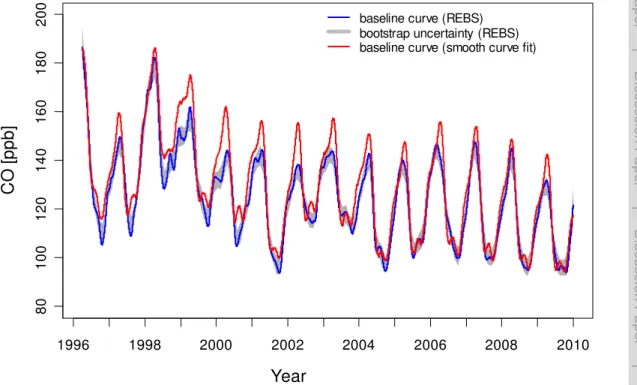
Figure 3 shows the estimated baseline curve for the REBS technique including the 95% bootstrap confidence band. As indicated in Sect. 2.2, the bootstrap confidence interval is asymmetric around the estimated baseline, the average width of the confidence band ranges from−3.5 ppb to 3.8 ppb. As the bootstrap confidence band indicates, some of the wiggles in the estimated background signal may not be statistically significant. This

20

may also mean that the true background signal is somewhat smoother than estimated by the REBS. Hence one might be tempted to increase the bandwidth h. However, a large bandwidthhhas the disadvantage of oversmoothing true temporal variability.

For comparison, the baseline curve obtained from the smooth curve fit is also in-cluded in Fig. 3. The baseline curve derived from the REBS technique is generally

25

(15)

AMTD

3, 5589–5612, 2010

Title Page

Tables Figures

◭ ◮

Back Close

Full Screen / Esc

P

a

per

|

Dis

cussion

P

a

per

|

Discussion

P

a

per

|

Discussio

n

P

a

per

|

during the cold period when background CO concentrations are highest. These dif-ferences would be of importance when emission estimates are performed using tech-niques as described e.g. by Reimann et al. (2005), Simmonds et al. (2001) and Greally et al. (2007) that are based on concentration above background estimates. However, the observed differences can be explained by the different methodical concepts

ap-5

plied: the REBS is a purely non-parametric technique that is capable to follow any long-term trend and seasonal variation. On the other hand, the smooth curve fit is less flexible: the parametric model fit given by Eq. (7) gives estimates for the long-term trend and the average seasonal variation of the observations. Superposition of the smoothed residuals allows for adjustment for temporary deviations from the long term

10

trend and for deviations from the average seasonal cycle, however, the main features of the course of the underlying parametric fit remains.

The linear trend of the CO background concentration was determined from regres-sion of the annual means of the identified CO background concentrations against time. The average annual change for the 1996 to 2009 period as determined from

15

the REBS filtered data is−2.1±1.3 ppb/yr, data filtering using the smooth curve fit re-sults in−2.3±1.3 ppb/yr, a slightly larger although not statistically significant di_fferent decrease of background CO (see also the study by Zellweger et al., 2009 for a discus-sion of the trend of CO at JFJ for the 1996 to 2007 period). Note that the linear negative trend of unfiltered hourly CO measurements for this time period is considerably larger

20

(−2.9±1.5 ppb/yr) due to more severe and more frequent pollution events during the first years of the considered time period (see Fig. 2).

5 Applicability of the REBS

As discussed in Sect. 4.1, trace gases (e.g. CO) can show latitudinal gradients due to the dependence of emissions and sinks on latitude. If strong latitudinal transport

25

(16)

AMTD

3, 5589–5612, 2010

Title Page

Tables Figures

◭ ◮

Back Close

Full Screen / Esc

Discussion

P

a

per

|

Dis

cussion

P

a

per

|

Discussion

P

a

per

|

Discussio

n

P

a

per

|

filtering methods including the REBS and most meteorological filters cannot correctly cope with the effect of latitudinal gradients. For the REBS, it is suggested that the residuals distribution as shown for CO at JFJ in Fig. 1 is used for judgment of the ap-plicability of the REBS for the time series of interest. The left hand site of the residuals distribution should approximately follow a Gaussian distribution. Obvious deviations

5

from this requirement indicate a significant impact of latitudinal transport or other pro-cesses leading to observations that are well below the background concentration at the sampling site. Observations well below the background concentration receive too high weights (see Eq. 4) and consequently lead to a baseline estimation that is biased downwards.

10

The REBS approach was recently extended by including the latitude of air mass ori-gin taken from back-trajectories as a second dimension in the local regression. This extended data filtering concept for estimation of background concentrations and lati-tudinal gradients of trace gases was denoted 2D-REBS and will be subject of a forth-coming publication.

15

A final issue to consider is missing data. The REBS technique can handle data gaps, whereas estimation of missing values and data interpolation is not recommended. In contrast to other techniques like running mean estimations, locally weighted regression as used in the REBS has no serious bias problems near the boundaries of data (Hastie et al., 2001).

20

6 Conclusions

A statistical method based on robust local regression is introduced. The presented REBS technique was applied for identification of background CO measurements at the high-alpine background site at Jungfraujoch, the results were compared to those from a more common approach denoted here as the smooth curve fit.

25

(17)

AMTD

3, 5589–5612, 2010

Title Page

Tables Figures

◭ ◮

Back Close

Full Screen / Esc

P

a

per

|

Dis

cussion

P

a

per

|

Discussion

P

a

per

|

Discussio

n

P

a

per

|

curves. The latter disagreement is explained by conceptional differences of the two methods. As a purely non-parametric approach, the REBS technique is more flexible than the smooth curve fit and can reproduce any long-term trend and highly variable seasonal cycles. In contrast, the smooth curve fit has limited capabilities to follow vari-ations in the seasonal cycle. Moreover, the smooth curve fit can only be successfully

5

applied to species with a long-term trend that can be described by a polynomial ap-proach as expressed by Eq. (7). If this is not the case, it might be difficult to find and to include an appropriate parametric function for estimation of the long-term trend. The REBS technique is certainly computationally more expensive and conceptually more complicated than the smooth curve fit. The above mentioned advantages of the REBS

10

should, however, outweigh these disadvantages in many applications.

Acknowledgements. The authors gratefully acknowledge the support from the International Foundation High-Altitude Research Stations Jungfraujoch and Gornergrat (HFSJG), and the custodians at the JFJ research station for their hospitality. The CO measurements at JFJ are part of the Swiss National Air Pollution Monitoring Network (NABEL) and supported by the

15

Swiss Federal Office for the Environment (FOEN).

References

Balzani L ¨o ¨ov, J. M., Henne, S., Legreid, G., Staehelin, J., Reimann, S., Prevot, A. S. H., Steinbacher, M., and Vollmer, M. K.: Estimation of background concentrations of trace gases at the Swiss Alpine site Jungfraujoch (3580 m a.s.l.), J. Geophys. Res., 113, D22305,

20

doi:10.1029/2007JD009751, 2008. 5591, 5600

Calvert, J. G.: Glossary of atmospheric chemistry terms – (recommondations 1990), Pure Appl. Chem., 62, 2167–2219, 1990. 5600

Carpenter, L., Green, T., Mills, G., Bauguitte, S., Penkett, S., Zanis, P., Schuepbach, E., Schmid-bauer, N., Monks, P., and Zellweger, C.: Oxidized nitrogen and ozone production efficiencies

25

(18)

AMTD

3, 5589–5612, 2010

Title Page

Tables Figures

◭ ◮

Back Close

Full Screen / Esc

Discussion

P

a

per

|

Dis

cussion

P

a

per

|

Discussion

P

a

per

|

Discussio

n

P

a

per

|

Cleveland, W. S.: Robust locally weighted regression and smoothing scatterplots, J. Am. Stat. Assoc., 74, 829–836, 1979. 5592, 5594

Cox, M. L., Sturrock, G. A., Fraser, P. J., Siems, S. T., and Krummel, P. B.: Identification of regional sources of methyl iodide from AGAGE observations at Cape Grim, Tasmania, J. Atmos. Chem., 50, 59–77, 2005. 5590

5

Derwent, R., Simmonds, P., O’Doherty, S., Ciais, P., and Ryall, D.: European source strengths and Northern Hemisphere baseline concentrations of radiatively active trace gases at Mace Head, Ireland, Atmos. Environ., 32, 3703–3715, 1998. 5591

Efron, B. and Tibshirani, R. J.: An introduction to the bootstrap, Chapman & Hall, New York, 1993. 5598

10

Fan, J. and Gijbels, I.: Local Polynomial Modelling and Its Applications, vol. 66 of Monographs on Statistics and Applied Probability, Chapman & Hall, New York, 1996. 5594, 5595, 5597 Forrer, J., Ruttimann, R., Schneiter, D., Fischer, A., Buchmann, B., and Hofer, P.: Variability

of trace gases at the high-Alpine site Jungfraujoch caused by meteorological transport pro-cesses, J. Geophys. Res., 105, 12241–12251, 2000. 5591

15

Greally, B. R., Manning, A. J., Reimann, S., McCulloch, A., Huang, J., Dunse, B. L., Sim-monds, P. G., Prinn, R. G., Fraser, P. J., Cunnold, D. M., O’Doherty, S., Porter, L. W., Stemmler, K., Vollmer, M. K., Lunder, C. R., Schmidbauer, N., Hermansen, O., Arduini, J., Salameh, P. K., Krummel, P. B., Wang, R. H. J., Folini, D., Weiss, R. F., Maione, M., Nick-less, G., Stordal, F., and Derwent, R. G.: Observations of 1,1-difluoroethane (HFC-152a) at

20

AGAGE and SOGE monitoring stations in 1994–2004 and derived global and regional emis-sion estimates, J. Geophys. Res., 112, D06308, doi:10.1029/2006JD007527, 2007. 5591, 5603

Hastie, T., Tibshirani, R., and Friedman, J.: The Elements of Statistical Learning, Springer Series in Statistics, Springer Verlag, New York, 2001. 5604

25

Henne, S., Furger, M., and Prevot, A.: Climatology of mountain venting-induced elevated mois-ture layers in the lee of the Alps, J. Appl. Meteorol., 44, 620–633, 2005. 5591

Holloway, T., Levy, H., and Kasibhatla, P.: Global distribution of carbon monoxide, J. Geophys. Res., 105, 12123–12147, 2000. 5601

Jacob, D. J.: Introduction to Atmospheric Chemistry, Princeton University Press, Princeton,

30

New Jersey, 1999. 5601

(19)

AMTD

3, 5589–5612, 2010

Title Page

Tables Figures

◭ ◮

Back Close

Full Screen / Esc

P

a

per

|

Dis

cussion

P

a

per

|

Discussion

P

a

per

|

Discussio

n

P

a

per

|

Novelli, P., Masarie, K., Lang, P., Hall, B., Myers, R., and Elkins, J.: Reanalysis of tro-pospheric CO trends: effect of the 1997–1998 wildfires, J. Geophys. Res., 108, 4464, doi:10.1029/2002JD003031, 2003. 5590, 5591, 5592, 5593, 5599, 5600, 5602

O’Doherty, S., Simmonds, P., Cunnold, D., Wang, H., Sturrock, G., Fraser, P., Ryall, D., Der-went, R., Weiss, R., Salameh, P., Miller, B., and Prinn, R.: In situ chloroform measurements at

5

Advanced Global Atmospheric Gases Experiment atmospheric research stations from 1994 to 1998, J. Geophys. Res., 106, 20429–20444, 2001. 5591, 5592, 5593

Prinn, R., Huang, J., Weiss, R., Cunnold, D., Fraser, P., Simmonds, P., McCulloch, A., Harth, C., Salameh, P., O’Doherty, S., Wang, R., Porter, L., and Miller, B.: Evidence for substantial variations of atmospheric hydroxyl radicals in the past two decades, Science, 292, 1882–

10

1888, 2001. 5590

R Development Core Team: R: a language and environment for statistical computing, R Foun-dation for Statistical Computing, Vienna, Austria, available at: http://www.R-project.org, last access: December 2010, ISBN 3-900051-07-0, 2010. 5593

Reimann, S., Manning, A., Simmonds, P., Cunnold, D., Wang, R., Li, J., McCulloch, A.,

15

Prinn, R., Huang, J., Weiss, R., Fraser, P., O’Doherty, S., Greally, B., Stemmler, K., Hill, M., and Folini, D.: Low European methyl chloroform emissions inferred from long-term atmo-spheric measurements, Nature, 433, 506–508, 2005. 5591, 5603

Ruckstuhl, A. F., Jacobson, M. P., Field, R. W., and Dodd, J. A.: Baseline subtraction using robust local regression estimation, J. Quant. Spectrosc. Ra., 68, 179–193, 2001. 5592,

20

5593, 5594

Ruckstuhl, A., Unternaehrer, T., and Locher, R.: IDPmisc: utilities of Institute of Data Analyses and Process Design (www.idp.zhaw.ch), available at: http://CRAN.R-project.org/package=

IDPmisc, last access: December 2010, r package version 1.1.08, 2010. 5593

Ryall, D. B., Maryon, R. H., Derwent, R. G., and Simmonds, P. G.: Modelling long-range

trans-25

port of CFCs to Hace Head, Ireland, Q. J. Roy. Meteor. Soc., 124, 417–446, 1998. 5591 Salibian-Barrera, M. and Zamar, R. H.: Bootstrapping robust estimates of regression, Ann.

Stat., 30, 556–582, 2002. 5598

Schuepbach, E., Friedli, T., Zanis, P., Monks, P., and Penkett, S.: State space analysis of changing seasonal ozone cycles (1988–1997) at Jungfraujoch (3580 m above sea level) in

30

Switzerland, J. Geophys. Res., 106, 20413–20427, 2001. 5590

(20)

AMTD

3, 5589–5612, 2010

Title Page

Tables Figures

◭ ◮

Back Close

Full Screen / Esc

Discussion

P

a

per

|

Dis

cussion

P

a

per

|

Discussion

P

a

per

|

Discussio

n

P

a

per

|

Weiss, R., and Prinn, R.: Global trends, seasonal cycles, and European emissions of dichloromethane, trichloroethene from the AGAGE observations at Mace Head, Ireland, and Cape Grim, Tasmania, J. Geophys. Res., 111, D18304, doi:10.1029/2006JD007082, 2001. 5592, 5603

Simonoff, J. S.: Smoothing Methods in Statistics, Springer Series in Statistics, Springer-Verlag,

5

New York, 1996. 5594, 5595, 5597

Thoning, K., Tans, P., and Komhyr, W.: Atmospheric carbon dioxide at Mauna Loa Observatory, 2. Analysis of the NOAA GMCC Data, 1974–1985, J. Geophys. Res., 94, 8549–8565, 1989. 5590, 5592

Yurganov, L. N., Duchatelet, P., Dzhola, A. V., Edwards, D. P., Hase, F., Kramer, I., Mahieu, E.,

10

Mellqvist, J., Notholt, J., Novelli, P. C., Rockmann, A., Scheel, H. E., Schneider, M., Schulz, A., Strandberg, A., Sussmann, R., Tanimoto, H., Velazco, V., Drummond, J. R., and Gille, J. C.: Increased Northern Hemispheric carbon monoxide burden in the troposphere in 2002 and 2003 detected from the ground and from space, Atmos. Chem. Phys., 5, 563–573, doi:10.5194/acp-5-563-2005, 2005. 5602

15

Zanis, P., Ganser, A., Zellweger, C., Henne, S., Steinbacher, M., and Staehelin, J.: Seasonal variability of measured ozone production efficiencies in the lower free troposphere of Central Europe, Atmos. Chem. Phys., 7, 223–236, doi:10.5194/acp-7-223-2007, 2007. 5591 Zellweger, C., Ammann, M., Buchmann, B., Hofer, P., Lugauer, M., Ruttimann, R., Streit, N.,

Weingartner, E., and Baltensperger, U.: Summertime NO_y speciation at the Jungfraujoch,

20

3580 m above sea level, Switzerland, J. Geophys. Res., 105, 6655–6667, 2000. 5599 Zellweger, C., Forrer, J., Hofer, P., Nyeki, S., Schwarzenbach, B., Weingartner, E., Ammann,

M., and Baltensperger, U.: Partitioning of reactive nitrogen (NO_y) and dependence on me-teorological conditions in the lower free troposphere, Atmos. Chem. Phys., 3, 779–796, doi:10.5194/acp-3-779-2003, 2003. 5591

25

(21)

AMTD

3, 5589–5612, 2010

Title Page

Tables Figures

◭ ◮

Back Close

Full Screen / Esc

P

a

per

|

Dis

cussion

P

a

per

|

Discussion

P

a

per

|

Discussio

n

P

a

per

|

Table 1.Contingency table of the classification of the hourly CO values measured at Jungfrau-joch from 1996 to 2009 (n=111 668) derived from the REBS technique and the smooth curve fit.

smooth curve fit background polluted

REBS background 102 405 0

(91.7%) (0.0%)

polluted 3188 6075

(22)

AMTD

3, 5589–5612, 2010

Title Page

Tables Figures

◭ ◮

Back Close

Full Screen / Esc

Discussion

P

a

per

|

Dis

cussion

P

a

per

|

Discussion

P

a

per

|

Discussio

n

P

a

per

|

(23)

AMTD

3, 5589–5612, 2010

Title Page

Tables Figures

◭ ◮

Back Close

Full Screen / Esc

P

a

per

|

Dis

cussion

P

a

per

|

Discussion

P

a

per

|

Discussio

n

P

a

per

|

(24)

AMTD

3, 5589–5612, 2010

Title Page

Tables Figures

◭ ◮

Back Close

Full Screen / Esc

Discussion

P

a

per

|

Dis

cussion

P

a

per

|

Discussion

P

a

per

|

Discussio

n

P

a

per

|

1996 1998 2000 2002 2004 2006 2008 2010

80

100

1

20

140

160

180

2

00

Year

CO

[

p

b

]

baseline curve (REBS) bootstrap uncertainty (REBS) baseline curve (smooth curve fit)