www.atmos-chem-phys.net/8/5669/2008/ © Author(s) 2008. This work is distributed under the Creative Commons Attribution 3.0 License.
Chemistry
and Physics
Origin of diversity in falling snow
J. Nelson
College of Science and Engineering, Ritsumeikan University, Nojihigashi 1-1-1, Kusatsu 525-8577, Japan Received: 20 December 2007 – Published in Atmos. Chem. Phys. Discuss.: 4 March 2008
Revised: 30 July 2008 – Accepted: 19 August 2008 – Published: 26 September 2008
Abstract. This paper presents a systematic way to examine the origin of variety in falling snow. First, we define shape diversity as the logarithm of the number of possible distin-guishable crystal forms for a given resolution and set of con-ditions, and then we examine three sources of diversity. Two sources are the range of initial-crystal sizes and variations in the trajectory variables. For a given set of variables, diver-sity is estimated using a model of a crystal falling in an up-draft. The third source is temperature-updraft heterogeneities along each trajectory. To examine this source, centimeter-scale data on cloud temperature and updraft speed are used to estimate the spatial frequency (m−1) of crystal feature changes. For air-temperature heterogeneity, this frequency decays asp−0.66, wherepis a measure of the temperature-deviation size. For updraft-speed heterogeneity, the decay is
p−0.50. By using these frequencies, the fallpath needed per feature change is found to range from∼0.8 m, for crystals near−15◦C, to∼8 m near−19◦C – lengths much less than total fallpath lengths. As a result, the third source dominates the diversity, with updraft heterogeneity contributing more than temperature heterogeneity. Plotted against the crystal’s initial temperature (−11 to −19◦C), the diversity curve is “mitten shaped”, having a broad peak near−15.4◦C and a sharp subpeak at−14.4◦C, both peaks arising from peaks in growth-rate sensitivity. The diversity is much less than previ-ous estimates, yet large enough to explain observations. For example, of all snow crystals ever formed, those that began near−15◦C are predicted to all appear unique to 1-µm reso-lution, but those that began near−11◦C are not.
Correspondence to:J. Nelson ([email protected])
1 Introduction
The deposition of water vapor in air produces crystals with a surprising degree of variety, symmetry, and intricacy. For-mation of various intricate features have been studied on-and-off over the years (e.g. Nakaya, 1954; Yamashita, 1976; Frank, 1982; Hallett and Knight, 1994; Nelson, 2005), and the symmetry is now understood to arise from the growth mode (Frank, 1982), but the sources of snow crystal variety have not been examined systematically.
The variety is generally equated to the number of possible crystal forms, a quantity that has been estimated through two approaches. The first approach is to estimate the number of possible distinct crystal forms for a given crystal radius (e.g. Knight and Knight, 1973). However, this approach yields no insights into the origin of the variety and it does not include limitations from the growth process; in particular, we neither learn the role of the crystal-growth response to the environ-ment nor do we see how this response may limit the types of crystal forms. A different approach was suggested much ear-lier by Bentley (1901) when he wrote that the various crystal features originate from the various “atmospheric layers” the crystal falls through1. As a preliminary step in this direction, Hallett (1984) used knowledge of the crystal response to es-timate the variety. His result, about 1030 000, is immense (and much less than the∼103 000 000of the first approach), but the method involved guessing the crystal’s environment. Now, 34 years later, we still do not know if crystals pass through enough “layers” (regions) to produce the observed variety, or even if those layers are the main source of variety. We address these questions here, and suggest that the answer to both is “yes”.
1He earlier used the more poetic expression “Was ever life
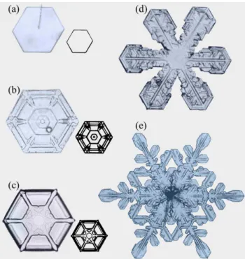
Fig. 1. Tabular snow crystals and their distinguishing features. Crystal(a)grew at low humidity near−9◦C in constant conditions, suspended by a capillary (radial line). The perimeter shows the six prism faces. Crystal(b)grew in free-fall under nearly constant con-ditions of−12.2◦C and liquid-water saturation (Takahashi et al., 1991). Crystals(c)–(e)are from natural snowfall. Distinguishing features of(a)–(c)are sketched, half-size, at right. Crystal(e)likely grew near−14◦C. All crystals viewed in transmitted light. Photos
(b)–(e)courtesy of Tsuneya Takahashi.
This paper described a growth-deviation model to system-atically examine contributions to snow-crystal variety from several sources. These sources are the initial states of a crys-tal, idealized (constant updraft) trajectories to cloudbase, and modifications to the trajectories from temperature and up-draft heterogeneities. By analyzing temperature and upup-draft- updraft-speed heterogeneities from recent cloud data, we derive an air-region thickness corresponding to Bentley’s layers. This “Bentley length”LB varies from about 0.8 m, when the air surrounding the crystal is near−15◦C, to 8 m near−19◦C, both of which are much less than the estimated crystal fall-paths of∼1800–2000 m for these temperatures. Thus, crys-tals should pass through enough regions to account for the variety. Of the three sources, the heterogeneities produced the most variety. The total value depends on the assumed resolution, but for micron-scale resolution, the variety is
∼10500, which is much less than previous estimates, though still immense. The results apply only to single crystals grown in relatively ideal conditions (yielding the more picturesque forms), but the model may be extended to irregular forms and more realistic conditions in typical snow clouds.
2 Diversity and growth
2.1 Shape diversity as the logarithm of variety
Regardless of how we estimate it, the variety, or number of possible distinguishable shapes, will be a very large number. For this reason, we instead work with shape diversityS, de-fined here as the base-10 logarithm of the variety. As such, the diversity is similar to entropy, which is proportional to the logarithm of the number of possible states instead of distin-guishable shapes2. The shape diversity has similarities and differences with the diversity that we perceive upon viewing snow. For example, both types of diversity will be large when crystals can grow in a wide range of conditions. But the di-versity we perceive in some crystal collection will depend on the degree and kind of differences between the crystals, not just on the existence of differences. However, this perceived diversity is hard to define unambiguously, whereas the shape diversity can be analysed mathematically. So, we analyze the latter in the hope that the results shed light on the former. 2.2 Distinguishing shapes
One can characterize a crystal shape by the dark lines in its image, lines that mark places where growth produced a sharp bend in the surface. For our purposes, these lines are the crys-tal features. For example, the feature of the cryscrys-tal in Fig. 1a is the perimeter, traced and scaled-down at right. Crystals in Fig. 1b and c have additional features in the interior, whereas crystals in Fig. 1d and e have more complex perimeter and interior features. Though it may help to picture the crystals from the viewpoint in Fig. 1, such a viewpoint is unnecessary for the analyses that follow. Moreover, even though “feature” is a crucial concept, a precise definition is not needed because we focus on growth-induced feature changes. These changes should be discernable in the following sense. If we resolve lines in the image to resolutionres, then any change in a sec-tion of line (including line splitting) by at least reswould be a distinguishable change. Thus, if two crystals follow paths that are identical, except that one experiences a change in conditions that produces a distinguishable feature change, then the two crystals would have distinguishable shapes. 2.3 Feature changes on single-crystal tabular forms In this paper, we treat only the growth of single-crystal tabular forms between ∼−9 and −22◦C. In this tempera-ture range, the prism-face growth rate is faster than that of the basal. This fact permits a major simplification – the assumption that most features arise from growth of the outermost prism faces. That the growth of these faces
2This similarity could be developed two ways: as part of a shape
(b)
(c) (a)
prism faces
(e) (d)
side rib
(f)
Initial temperature
Back to initial temperature Deviation away from ~ – 15 °C
Lateral case Normal case
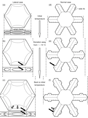
Fig. 2.Two examples of crystal feature changes from temperature changes in a cloud at liquid-water saturation. Left column (top to bottom) shows a feature change on a hollow plate due to growth lateral to the prism axes.(a)is the initial crystal. Front view below the sketch shows the pits in the three prism faces. In(b), growth slows asT moves away from the growth-rate peak near−15◦C, narrowing the lip of the pit (filled arrow). In(c), growth resumes at the faster rate asT returns to its previous value, thus widening the lip of the pit (filled arrow). Grey lines are feature changes due to the growth-rate change, here boundaries of the pits and ribs (hollow arrows). Right column shows a feature change on a stellar crystal due to growth normal to the prism axes.(d)is the form from growth under constant conditions. Side ribs and the longer main ribs are ridges on the branch underside (Nelson, 2005). Growth slows in
(e), asT moves away from the growth-rate peak, widening the tip (solid arrow), before resuming at the faster rate, at the previousT, and narrowing in(f)(solid arrow). Hollow arrows mark the feature changes in both cases. If growth had not slowed, the features would instead follow the dashed lines.
controls the perimeter of a simple, solid hexagonal plate (e.g. Fig. 1a) needs no explanation. But the growth history of these faces should determine other feature changes too. For exam-ple, in the case of a hollow plate (Fig. 2a–c), when the prism-face growth temporarily slows, the hollows can decrease in size, producing a wiggle in an “interior” line and the split-ting of the perimeter line shown in the figure. For the case of a stellar crystal, a similar growth-rate change can produce a ‘band’ on each branch (Fig. 2d–f). A recent study of various
-18 -16 -14 -12 0
0.2 0.4 0.6 0.8 1
1.05
r [μm/s]
T [°C]
-14.8
growth rate r = dR/dt
v [m/s]
0.15
0.20
0.25
0.143
dR
crystal fallspeed v
Fig. 3. Prism-face growth rates (left axis) and fallspeeds (right axis) for crystals grown at constant temperature. Curves are fits to Takahashi et al.’s (1991) data for crystals grown for 10 min. At later times,vincreases, most rapidly at temperatures away from the peak, andrdecreases slightly, mainly at temperatures away from the peak. (Functional forms are in Appendix C.) Marks on the abscissa mark peaks inr’ and r. The basal-face growth rate (not shown) has a minimum where the prism-face has a maximum.
observations suggested how other common features likely arise from prism-face growth-rate changes (Nelson, 2005).
2.4 Prism-face growth changes from temperature changes The prism-face growth rate r generally depends on crys-tal size and shape, air pressure, vapor pressure, and tem-perature. However, sufficiently extensive data are available only for constant-temperature measurements of growth un-der conditions of atmospheric pressure and a vapor pres-sure equal to equilibrium over pure liquid water. Luck-ily, these are typical conditions in snow-producing clouds. Snow-producing clouds often contain significant liquid wa-ter over much of their lifetime. In such mixed-phase con-ditions, measurements (Korolev and Isaac, 2006; Siebert et al., 2003)3 and theory (Shaw, 2000) suggest that the vapor pressure stays near liquid-water saturation. Hence, we will assume that the ambient vapor pressure is at the temperature-dependent liquid-water saturation value. This will greatly simplify the treatment, but we should remem-ber that the results will only apply to such liquid-rich con-ditions. Moreover, we will ignore crystal-crystal collisions and effects from the close passage of, and collisions with, droplets. Finally, as no measurements of polycrystal growth rates are available, the model is restricted to single crystals. With these assumptions, the air temperature T controls r. This rate has a peak near−14.8◦C (Fig. 3), which suggests
3In the former, measurements were averaged over 100 m. In the
crystal history t
0
ū
v
dz
dt T 0 + δT0 ū + δū
ū+ Du(t)
δT0 ΔT0
df, Lf
ΔTf δTf δd0
Δd0 δū
initial crystal {d0}
reference trajectory {T0, ū, Tf}
temperature deviations {DTTh, DTDu}
+ +
T0
Tf
-23 °C
z
0 °C crystal height
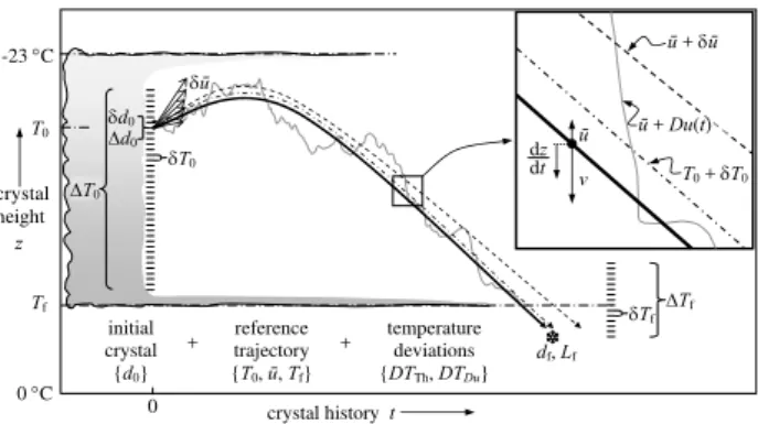
Fig. 4. Overview of growth-deviation model. In a trajec-tory z(t ), a crystal nucleates with diameter d0 at T0 in an up-draft u¯ then falls at speed v− ¯u until reaching cloudbase at temperature Tf (solid curve). Each resolvable variation δd0,
δT0, δu¯, and δTf results in a final diameter df that changes
by ±2•res (dashed curves). Variable ranges are 1d0, 1T0,
1u¯, and 1Tf, making the number of distinct reference classes
N0•Nref=(1d0/δd0)•(1T0/δT01u/δ¯ u1T¯ f/δTf). Values are in
Table 1. DTT handDTDu(from updraft deviationsDu– dotted
curve) are temperature deviations that further alter crystal shape. For each trajectory, the numberNdev of deviation-caused shape changes depends ondf/res, the final pathlengthLf, and the
num-ber of relevant deviations/meter (FT h+FDu).
that we must carefully track the temperature to estimate when distinguishable changes to growth features can occur.
3 Crystal trajectories and diversity sources
Withrdepending only onT, the initial crystal properties and temperature history determine the final crystal form. We now study these influences in detail.
3.1 Initial crystals and reference trajectories
Most snow crystals start as frozen droplets. Subsequent growth may be affected by various crystalline imperfections from the freezing process, but the effects are poorly under-stood4. So, we characterize the initial crystal by its diameter
d0. The initial temperatureT0is also an initial characteristic,
but we instead useT0as a trajectory parameter.
Temperature changes along a crystal trajectory are due to spatial air-temperature heterogeneityDTT h, which exists at a fixed time, and the altitude-dependent air temperature in the absence of temperature heterogeneity, which occurs during
4Under slow growth conditions, dislocation outcrops on the
sur-face influence growth. During freezing, chemical impurities may lead to dislocations or produce other surface effects. Also, larger drops are more likely to freeze with internal stresses and become polycrystals, particularly at low temperatures.
Table 1.Trajectory results fordf,Lf,S0, andSref.
T0[◦C] −11 −13 −15 −17 −19
dfa[µm] 441 1843 7600 3919 2069
Laf[m] 686 1227 1850 1866 2009
δd0a[10−7m] 96 52 38 2.9 3.2
δT0a[10−3◦C] 9.1 1.4 1.5 1.2 4.4
δu¯a[10−5m/s] 110 27 5 25 100
δTfa[10−2◦C] 4.3 2.8 2.2 5.1 10
Sb0 0.7 1.0 1.2 1.5 1.5
Sbref 7.5 9.3 10.1 9.1 7.5
aBaseline case (1 below),res=1µm. (cloud is 2143-m thick). bAverage of cases 1–4: {d
0[µm],u¯[m/s],Tf[◦C]}=1: {8, 0.12, −8}; 2:{1, 0.12,−8}; 3:{1,0.01,T0+1}; 4:{40, 0.25,T0+11}.
the crystal’s up-down motion. The latter is the sum of that from 1) slowly varying altitudes for a crystal in an updraft of constant speed, and 2) heterogeneityDTDufrom altitude deviations due to updraft-speed deviationsDu. Horizontal motion is ignored.
To account for these temperature deviations, we write the crystal temperature at timet as T (t )=T (z(t ))+DT (t ), whereT (z(t ))is the temperature for a crystal lofted in an up-draft with the cloud-averaged speedu¯, in which the altitude is
z(t ), andDT (t) is the total temperature deviation along a tra-jectory (=DTT h+DTDu). A given trajectoryz(t ), hereafter a “reference” trajectory, changes asdz/dt= ¯u−v, wherev
is the crystal’s terminal fallspeed andT (z)decreases withz
asdT (z)/dz≡T’=−7×10−3◦C/m, a typical environmental
lapse rate. An actual updraft has speedu¯+Du(t ), butDuis used only to estimateDTDu, not for calculating trajectories. These and other model parameters are sketched in Fig. 4 and a full listing of symbol definitions is in Appendix A.
The duration of a trajectory depends on T0, Tf, u¯, and how quicklyv increases. The fallspeed depends on crystal shape, and increases slowest for the crystals that grow the fastest (Fig. 3). These crystals fall slowest because, as tab-ular crystals fall broadside to the airflow, the broadest (and thinnest) crystals expose the greatest area to the airflow, and thus have the greatest drag force. Hence, the crystals that grow the fastest also fall the slowest, and end up with the longest growth times.
3.2 Three sources of diversity
A reference trajectory begins when a crystal nucleates at tem-peratureT0from a droplet of diameterd0. Here−11≥T0≥ −
Whenvreachesu¯, the crystal has its maximum altitude5and minimum T, and thereafter falls towards cloudbase at the warmer temperatureTf where growth is assumed to stop. (Growth below cloudbase is ignored, even though the vapor pressure exceeds ice saturation for some distance.) The tem-perature deviations then superimpose on the reference trajec-tories. During such a history, the origin of crystal variety can be divided into three sources: variations in the initial diame-ter, variations in the reference trajectory, and temperature de-viations due to cloud heterogeneities. From these varieties, the corresponding diversities are calculated.
Each source is treated separately. LetN0be the number
of possible forms due to variations of the initial crystal di-ameter, a number that will generally depend on the reference trajectory. Similarly,Nref is the corresponding number for
the reference trajectories, and may depend on the initial di-ameter, whereasNdevis the corresponding number for
devi-ations. Ndevwill generally depend on the initial crystal size
and trajectory parameters. The shape diversities from these influences
S0=log10[N0],
Sref=log10[Nref], and
Sdev=log10[Ndev], (1)
are evaluated next.
4 Variations of initial crystal and reference trajectories
To evaluate S0, Sref, and Sdev, we use the numerical
inte-gration method in Appendix B to track the crystal diameter
d(t ), temperature T (t ), and pathlength L(t ) (air depth the
crystal falls through) for timet along reference trajectories. First, we use the reference trajectories to analyzeS0andSref.
A trajectory is determined byd0,T0,Tf,u¯, andv. Butv depends ond0andT (t )through the crystal size and shape.
Thus, reference trajectories depend only on d0,T0, u¯, and
Tf. Upon exiting cloudbase, the crystal has diameterdf and total pathlengthLf.
4.1 Distinguishable reference classes for trajectories with-out deviations
Consider a reference trajectory with some values ofd0,T0,
¯
u, and Tf, but one variable, say u¯, is varied by du¯. For all|du¯|less than some value, defined asδu¯, the final crys-tal forms will be indistinguishable. (Ignore cloud hetero-geneities for now.) When|du¯|>δu¯, the resulting crystal will have some feature displaced by at leastresfrom that on the original (|du¯|=0) crystal. To determineδd0, δT0, δu¯, and
δTf, we consider changes todf, a common feature that is relatively sensitive to the temperature history. Thus, if vari-ableX with valuex results indf, then valuex+δXresults
5For updrafts considered here, the altitude increase is typically
less than 100 m.
indf±2•res. So, ifdf is sensitive toX, thenδXwill be rel-atively small. Crystals withind0±δd0/2,T0±δT0/2,u¯±δu¯/2,
andTf±δTf/2 are said to be in the same “reference” class; they can have complex features, yet would be observed as indistinguishable.
4.2 Number of reference classes
To estimate S0 and Sref, we need a typical range of each
variable. Call these 1d0, 1T0, 1u¯, and 1Tf. The re-sulting number of possible distinguishable crystals due to changes ind0isN0=1d0/δd0, though this number will
de-pend somewhat on the values of d0, T0, u¯, and Tf used to calculateδd0. The corresponding numbers for the other
variables are 1T0/δT0, 1u/δ¯ u¯, and 1Tf/δTf. We as-sume that d0 varies between 1 and 40µm, T0 varies
be-tween−10 and−20◦C,u¯ varies between 0.01 and 0.25 m/s, andTf (always>T0) varies between−9 and−17◦C. Thus
{1d0, 1T0, 1u, 1T¯ f}={39µm, 10◦C, 0.24 m/s, 8◦C}. Use of the calculated trajectories showed that the diver-sitiesS0 andSref depended ond0, T0, u¯, and Tf, with the greatest dependence being onT0. Averaging over the results
from fiveT0(Table 1) givesS0=1.2 andSref=8.7.S0is small
becaused0has a significant influence only at the start; for
ex-ample, a crystal that begins 2-µm larger will end about 2-µm larger. This suggests thatS0≈log10[1d0/2•res]=1.3. The
value is instead 1.2 becaused also affectsv. Sref is much
larger, mainly because df is sensitive toT0 andu¯, both of
which affectT (and hencer) throughout the trajectory. In contrast,Tf only affectsLf, thus adding relatively little to
Sref.
5 Temperature deviations due to cloud heterogeneities
A given reference class represents a certain shape. We do not know this shape, but we nevertheless can consider pos-sible variations to the shape, variations that arise from air-temperature and updraft-speed heterogeneities along the fall-path. As a crystal falls, the heterogeneities produce a contin-uously varying DT that alter the crystal’s growth features. But there will be some average duration between relevant
DT changes, that is, betweenDT changes that can produce distinguishable changes to the crystal features. As there can be many possible sequences of relevant changes, each refer-ence class can contain many possible crystal forms.
5.1 Number of relevant deviations
We set a growth-amount criterion for the relevant devia-tions, then estimate how often the criterion is satisfied for a given crystal path. In timedt, a crystal falls through path-length dL=v dt as its outermost prism faces advance by
dR=r dt, where r is the prism-face growth rate (Fig. 3). (dL6=dzunlessu¯=0.) A temperature differing byDTi pro-duces a growth-rate changedri=r’DTi, wherer’≡dr/dT is the growth-rate sensitivity and “i”=“T h” or “Du”. The size of the surface perturbation thus produced is d2Ri=dridt. (For a lateral deviation (e.g. Fig. 2a–c), the growth rate is un-known, so we useras an approximation.) Integratingd2Ri between depthLt at timet andLt+Lat timet+L/vgives
δRi:
δRi(Lt, L)=
Z Lt+L
Lt
r′(x)DTi(x)v−1(x)dx
≡r′v−16i(Lt, L), (2)
where the T changes are small enough to remover’andv
from the integrand. The number of relevant deviations in6ι is nearly independent ofLt, so we will ignore this depen-dence. For a surface perturbation to enlarge, it must receive more vapor flux than adjacent regions. To do so,δRmust ex-ceed the vapor mean-free pathλ, which we fix at 0.08µm (λ
varies only slightly withT andz). Assuming that the pertur-bation continues to grow, eventually exceedingres, the per-turbation from Eq. (2) can change a feature when
6i(L)≥
λv
r′≡p. (3)
The parameterpgreatly influencesSdevdue to the
sensi-tivity ofvandr’ toT. During growth,pgenerally increases due to the increase of v. For crystals with T0=−15◦C,
p increases slowly, and much of the growth occurs with
p∼0.018◦C m. In contrast, crystals with T
0near −11 and
−19◦C have faster-rising values ofpthat average about 10 and 20 times larger.
5.2 Distribution functions from stratus clouds
The number of times that Eq. (3) is satisfied depends onp
andL. To handle this dependence, we define peak distri-bution functions Fi(p) as the number of peaks exceeding
p in unitL. To estimate Fi(p), I used data from horizon-tal flight paths in stratus clouds withT <0◦C. The values of
DTT h were direct measurements, but DTDu required inte-gration ofDuto get the altitude deviationDz, from which
DTDu=T’Dz. (The integration introduced factorv−1 into
δRDu, and thusFDu also depends onv.) Then I integrated
DTi to obtain6i, from which theFi were derived. Details are in Appendix D.
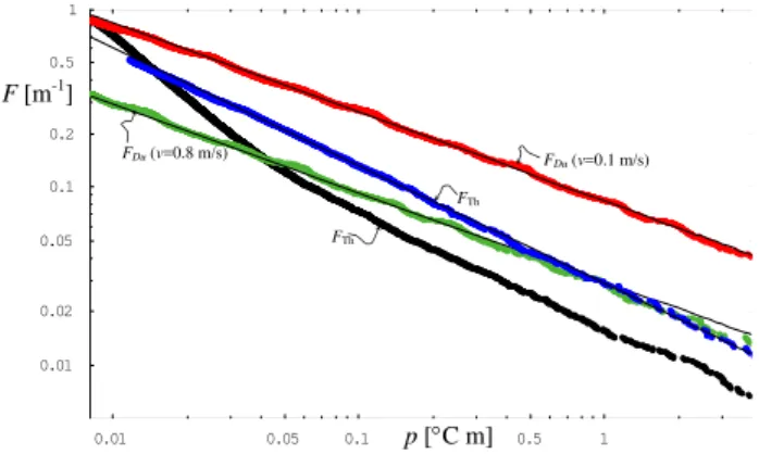
The FT h functions from two cloud datasets decayed as
p−0.66 and agreed within a factor of two, even though the
0.01 0.05 0.1 0.5 1 0.01
0.02 0.05 0.1 0.2 0.5 1
FTh
FTh
FDu (v=0.1 m/s)
FDu (v=0.8 m/s)
p [°C m]
F [m-1]
Fig. 5.Temperature deviation distribution functionsFT handFDu.
All functions are from measurements at 15-cm intervals except the lowerFT hone, which instead had 8-mm intervals. Also shown are
fitsFT h=0.0287p−0.66andFDu=0.0262p−0.50v−0.5.
clouds had different temperature averages and the measure-ments were done differently (Fig. 5). In contrast, only one cloud dataset was available forFDu, and the values decayed asp−0.50. The reasonFidecay with increasingpis because larger temperature deviations are rarer, but the reason for ex-ponents−2/3 and−1/2 is unclear.
The reciprocal of the sum of the distribution functions is the fallpath needed for a feature to form. This distance is analogous to the layer thickness mentioned by Bentley (even though “layer” suggests homogenous, horizontally extended regions, neither of which may occur). To acknowledge his insight, let us call this the Bentley lengthLB:
LB(p, v)≡
1
FT h(p)+FDu(p, v)
. (4)
Using the estimated minimum p of 0.018 with v=0.1 m/s, which applies to a small crystal growing near−14.8◦C, the total value ofF is ∼1.2 m−1, making LB∼0.8 m. In con-trast, a maximumpof 0.36 withv=0.4 m/s (appropriate for a large crystal near−19◦C) givesL
B∼8 m. Most values of
LBshould lie in between these extremes. 5.3 Number and positions of feature changes
For constantpandv, the number of timesnthat a temper-ature deviation can change a fetemper-ature is the ratio of the total pathlength with the Bentley length. But only some fraction
χ of the deviations will grow into a distinguishable feature change, so
n= χ Lf
LB(p, v)
. (5)
Each of these feature changes could have been born when the outermost prism faces were at any one ofmdistinct ra-dial positions on the crystal. As these will be separated by intervals ofres, we have
m= df
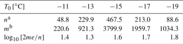
Table 2.Combinatorial parametersnandmforSdev.
T0[◦C] −11 −13 −15 −17 −19
na 48.8 229.9 467.5 213.0 88.6
mb 220.6 921.3 3799.9 1959.7 1034.3
log10[2me/n] 1.4 1.3 1.6 1.7 1.8
aBased onL
f from Table 1, and the averageFT h+FDufor the
coldest and warmest parts of the trajectory.
bm=d
f/2res, withdf from Table 1.
That is, there aremresolvable growth intervals.mandnare used below to calculateSdev. Althoughmdepends on both
the resolution and trajectory (throughdf),ndepends only on the trajectory.
5.4 Estimates ofLf,df,m, andn
The reference trajectories were used to estimateLf anddf (Table 1), and then mandn. The values of Lf increased asT0decreased because the distance to cloudbase increased,
but the increase is most rapid asT0approaches−15◦C from
lower heights due to the decrease inv (Fig. 3). The value ofLf could greatly exceed the cloud thickness whenu¯was large (≥0.25 m/s) and T0 was near −15◦C (where v was
small), but even at other values ofu¯andT0, the value greatly
exceededLB. LikeLf, the diameterdf initially increases asT0decreases, but in contrast,df decreases above−15◦C. This peak is due to both the maximum inrand the minimum inv. From Eq. 6, mhas an analogous peak. Then maxi-mum near−15◦C (Table 2) also has two causes: the trend inLf and the peaks in r’ at −14.0 and −15.4◦C (Fig. 3) that greatly decreaseLB. In Sect. 6.2 below, we integrate
dn=dLχ /LB(p, v)for more precise analysis and show that
a double-peak exists.
5.5 Combinatorial method forSdev
Within a reference class, a crystal hasnfeature changes that can arise inmgrowth intervals, each of which may be born during either a growth spurt or lull, meaning that each inter-val can develop one of two possible feature changes6. The resulting number of feature-change combinations is an ap-plication of a common calculation (Feller, 1968):
Ndev=
m n
2n= m! n!(m−n)!2
n.
(7)
6Onlym≥nmakes sense, sonmust be limited tom. Ifres
ex-ceeds about 5µm,n>mfor some conditions and the analysis be-comes more involved, though one could argue that the RHS of Eq. 7 becomes 2n.
-18 -17 -16 -15 -14 -13 -12 -11 100
200 300 400 500
Sdev
baseline
ū = 0.12, 0.06, 0.03 [m/s]
Tf = -8, -10, T0 + 1 [°C]
χ = 1/2, 1/4, 1/8
res =1, 2, 4 [μm]
χ =1/8
Tf = T0 + 1
m/30
n/3
T0 [°C]
Fig. 6. Shape diversitySdev. The upper black curve, the baseline case (bold values in legend), is derived from the grey curves ofm (reduced 30-fold) andn (reduced 3-fold). Solid triangles, stars, squares, and diamonds mark peak positions for other values ofu¯, Tf,χ, orres. Full curves show casesχ=1/8 andTf=T0+1.
Verti-cal lines on the abscissa are peak positions and relative magnitudes for the baseline case (black lines), the value ofm(long grey line), and the value ofn(short grey lines).
Asm≫1,n≫1, andm−n≫1 (Table 2), Stirling’s factorial approximation can be used:
Ndev≈
2n
q
2π n(1−mn)
(mn−1)n
(1−mn)m. (8)
Whenm≫n,Ndevapproaches (2π n)−1/2(2me/n)n, showing
thatNdev increases rapidly when eithermornincrease. In
this case
Sdev≈n·log10[
2m·e
n ]−
1
2log10[2π n]. (9)
Whenres<4µm, Eq. (9) is accurate to within 1–3% of the
value derived from Eq. (7).
6 Discussion
6.1 Cloud heterogeneities as the main source of diversity As log10[2me/n]>1 andn≫1/2 (Table 2), Eq. (9) suggests
thatSdevexceedsn, which exceedsS0+Sreffor allT0.
Fur-ther analysis of the dependence ofS0,Sref, andSdev onres
6.2 Further examination ofSdev: the “mitten” curve
A plot of Sdev versus T0 reveals a curve in a mitten-like
shape (Fig. 6). Specifically, for most cases considered, the curve has a larger, broader peak near−15.4◦C and a smaller, narrower peak near −14.4◦C. The two peaks come from
n, which is double-peaked becauser’ has maxima on both sides of the growth-rate peak near −14.8◦C. The lower-temperature peak ofSdevis larger partly because only
lower-temperature crystals experience bothr’ maxima during their descent. In addition, crystals that start at lower temperatures have greaterSdevdue to their largerdf, which is partly due to their longerLf. These asymmetries are greatly reduced when the cloudbase is only 1◦C warmer thanT0, making the
curve more nearly symmetric about the growth rate peak. To better understand theT0dependence, consider how the
crystal-growth propertiesr,r’, andvaffectSdev. In the
base-line case,Sdevchanges from 41.3 at−11.0◦C to 479.9 near
−15.4◦C, an increase of 438.6. But when theT0= −11◦C
case was run withr(T )evaluated 4.4◦C lower (to equal that of a −15.4◦C crystal), the resulting Sdev was 64.0, an
in-crease of 22.7. If insteadv was evaluated 4.4◦C lower, the value ofSdevincreased by 33.4. However, whenr’ was
eval-uated 4.4◦C lower, Sdev increased by 60.2, the largest
in-crease7. Therefore,v had a larger effect onSdev thanr, but
r’ had the largest effect.
In nature, the biggest crystals are usually observed to be the most elaborate. This observation can be explained as a combination of two factors. One,Sdevincreases with the
fac-torm, which is largest for the largest crystals (Eq. 9). Two, the peaks inSdev are mainly due to the nearby peaks inr’
and the minimum inv, both of which are either close to or at the maximum inr, and these conditions (larger, smallv) are exactly the conditions that produce the largest crystals. Therefore, large crystals form under nearly the same condi-tions that are needed for maximum diversity.
6.3 Sensitivity and uncertainty inSdev
Sdev was relatively insensitive to Tf but sensitive to u¯. A decrease inTf decreased Sdev for all crystals, particularly
those that started near cloudbase. But the decrease is rela-tively small, and peak temperatures shifted only slightly to higherT0(Fig. 6, stars). The latter occurred because a
rais-ing of cloudbase decreasesLf. A greater decrease inSdev
occurred whenu¯decreased to 0.03 m/s. In this case, the peak temperatures shifted to lowerT0. The lower values are due to
the shorterLf, and the decrease in peak temperatures occur becauseT0 must decrease to have the same minimum
tem-perature, where much of the growth occurs.
7The sum of the individual effects is 116.3, much less than the
curve’s 438.6. This difference is becauseSdevdepends nonlinearly
on r, r’, and v. When all three parameters were 4.4◦C lower, Sdevincreased by 366.1. The remaining difference is because the
−11.0◦C case is closer to cloudbase.
In contrast,Sdevwas sensitive toresandχ. If the
resolu-tion is coarser, thenresis larger and the diversity is less. For example, Fig. 6 shows that the peak diversity decreases by about 170 whenresincreases from 1 to 4µm. This decrease is due to a decrease in m. Even greater sensitivity comes fromχ due to the proportionality of ntoχ. For example, when χ decreased from 1/2 to 1/8, the peak diversity de-creased from 486 to 160. The valueχ=0.5 used in the base-line case is uncertain and likely depends on crystal form, fea-ture type, and the size and rate of the deviation. Qualitatively,
χ should be relatively large near peak growth rates, due to the step-clumping that leads to various feature changes (Nel-son, 2005), yet may be nearly zero for small, slow-growing crystals that have not yet hollowed (e.g. Fig. 1a). So,χ=0.5 may overestimateSdev, at least at slow growth rates, though
its functional form and numerical value remain highly uncer-tain. Whenχ becomes better known, it can be inserted into the present model.
6.4 Neglected influences on diversity
The vapor pressure in a cloud cannot always be exactly at liquid-water saturation. For example, in a updraft, a re-gion devoid of droplets will be slightly supersaturated (Shaw, 2000), whereas a similar region in a downdraft will be under-saturated. Also, entrainment of subsaturated air can create subsaturated regions. Moreover, if nearly all of the droplets freeze, the vapor pressure can decrease to near ice saturation. Unfortunately, we have no fine-scale data on vapor-pressure deviations from liquid-water saturation. When such data be-come available, we could use the same method as that used here forT. In particular, Eqs. (2) and (3) would apply, with the necessary substitutions, giving rise to a third distribution function that would appear as a third term in the denomina-tor of Eq. (4). As a result,LB would decrease andnwould increase, thus increasing Sdev. However, unlikeT,
vapor-pressure has no altitude term, which is large in the tempera-ture case: FDu>FT hfor a range ofv (see Fig. 5). The lack of an altitude term would reduce their contribution, though vapor-pressure heterogeneities may still add much diversity.
Other potentially major sources of variety are the initial crystal’s structure and close passages/collisions of droplets. When the growth rate is low, step-producing defects can greatly affect the growth rate of a prism face (Wood et al., 2001). Moreover, crystals nucleated under different condi-tions can end up with different shapes (Yamashita, 1973). But we have little knowledge of either influence. Also, droplets may pass close to, and land on, a crystal, thus lo-cally changing the humidity and temperature. For example, the droplet density can affect the growth rate (Takahashi and Endoh, 2000; Castellano et al., 2007) and cause clear feature changes in some cases (Hallett and Knight, 1994), though quantitative treatment is not presently possible.
diversity is most sensitive to the growth-rate sensitivityr’. But for the temperature range considered here, the basal face growth rate is relatively insensitive to temperature. For example, between about −11 and −15◦C, the basal-face growth rate changes by only about 0.025µm/s, much less than the corresponding 0.9µm/s of the prism-face (Taka-hashi et al., 1991). The sensitivities of the two faces are more nearly the same near the tabular-columnar transition temperatures (near−9 and−23◦C), but feature changes are relatively rare at such temperatures. At other temperatures, the basal face might have relatively little direct influence on the diversity.
6.5 Errors from using non-ideal datasets
Model results are based on the available data, which, unfortu-nately, are not perfectly suited for applications to real crystal trajectories in snow clouds. Three problems are mentioned here. One, although crystals fall vertically through the air currents, the only available data on temperature and updraft heterogeneity are from measurements along near-horizontal flight paths. If, for example, the temperature deviations along a vertical path are more spread out than they are along the horizontal and the distribution function has the same power-law scaling, then one can show that the distribution functions would be smaller. Two, snow clouds can have regions with values ofu¯much larger than the values here (Wolde and Vali, 2001). However, larger values ofu¯would produce unrealis-tically large crystals, so the baseline-caseu¯ here may be a reasonable average. Three, data onr andvcover only ide-alized, constant conditions, and even in these conditions are imprecisely known. For example, more recent, yet limited, data suggest that the growth-rate peak is flatter on top than that shown in Fig. 3 (Takahashi et al., 2008). However, such a change would not alter the main findings here. Finally, in an actual cloud, side-to-side (leaf-like) falling motion and changing temperatures may alterr andv. These considera-tions show that new measurements of cloud and snow-crystal growth properties are needed to advance our modelling of snow-crystal diversity.
6.6 The total diversity
Because all three sources of diversity, particularlySdev, vary
with the crystal-cloud variables, the total diversityStotis not
a simple sum ofS0,Sref, andSdev. Rather, an accurate
es-timate ofStot would involve calculating the logarithm of a
sum ofNdevover the reference classes. Instead of
attempt-ing such a sum, we estimate an upper limit toSas the sum of the maximum values ofS0,Sref, andSdev. Forχ=1/2and
res=1µm (a relatively high optical-microscope resolution), this upper limit is 1.5+10.1+475≈487. Given the various un-certainties involved and neglected influences on diversity, the actual number may be larger by several orders of magnitude.
Nevertheless, unlessχexceeds1/2near−15◦C, then an up-per limit to the total diversityStotshould be about 500.
6.7 Comparison to previous estimates
The upper limit Stot∼500 is large, yet much less than
pre-vious estimates. Knight and Knight (1973) estimated the number of molecules in a typical snow crystal and then considered, but did not evaluate, the number of ways these molecules could be arranged. A lower bound of this num-ber is derived from Eq. (6) by substituting for m a crys-tal radius divided by the water-molecule diameter and sum-ming over alln(0 tom). The result is 3m, which, for a ra-dius of 3 mm, givesStot∼3×10⁶. In contrast, Hallett (1984)
assumed a resolution 3×10⁴times larger (10µm), yet
cal-culated Stot∼5×10⁶. His estimate involved consideration
of 104 “points” on the crystal, apparently each of which could have grown in one of 20 humidity classes and one of 50 temperature classes. (S0was ignored.) Based on these
as-sumptions, the number of possible crystals should instead be (20×50)10 000, which givesStot=3×10⁴. Regardless of their
differences, these previous estimates are vastly larger than the Stot found here, and this is mainly because limitations
from the growth process were not included. This huge differ-ence in numbers has implications for the following question. 6.8 Comparison to observations: should every snow crystal
look unique?
An observational test of the mitten curve is impractical unless resis very large. So instead, we check to see if the numbers are reasonable by estimating the likelihood that all crystals in a collection appear unique.
Consider a large, heavy snowstorm that deposits a liquid-water-equivalent snow depth of 3 cm (∼50 cm of snow) over a land area of 104km2. In total, this equals∼3×10¹¹kg of water, which, if each crystal is 10−9kg, amounts to∼3×10²⁰ crystals, of whichNc∼3×10¹⁸ may have been reasonably symmetric at cloudbase8. This number could be compared to the total variety∼10Stot; however, the variety of one ref-erence class can be many orders of magnitude different from another. So we instead consider each reference class sepa-rately.
8Highly symmetric crystals (at typical viewing resolution) are
unlikely. For example, Korolev et al. (1999) found that only∼3% of the sampled crystals were “pristine”. But we could average the features over the twelve 30◦sectors, one bisector along the center of each branch. Or, we could consider each sector independently, and find the probability that any two, out of all 12Ncof the sectors,
p1
p2
0 200 400 600 800 1000 a
b
c
d 1.0 1.2 1.4
0 0.016
0 0.032 -7.6
-7.7
-0.008
TTh
[°C]
u
[m/s]
ΣTh
[°C m]
-0.016
ΣTh ´
[°C m]
Fig. 7. Analysis of deviations.(a)Segment ofTT hdata.(b)
Seg-ment ofu¯+Dudata. (c)Integrated temperature6T hfrom section (a). Maximum peakp1is marked. (d)6T hafter the peak in(c)
was removed by breaking the segment into pre-peak and post-peak segments as described in Appendix D. New maximum peakp2is
marked.
To estimate crystal uniqueness, we assume the crystals are equally likely to be in each class. As a result, the number of crystals per classNcclisNcdivided by the number of classes, orNc/10S0+Sref. Using the averageS
0andSreffrom Table 1,
Nccl=4×10⁸. (As this exceeds unity, there would be many
identical crystals if heterogeneities did not exist.) The prob-ability pd(i)that all crystals in class i are distinct can be estimated by counting the number of ways that this class can have only distinct crystals. This problem is equivalent to the “birthday paradox” problem, which is the surprisingly low probability that all people in a group have birthdays on dif-ferent days of the year. AsNccl≫1 andNdev(i)≫1, we can
use Feller’s (1968, end of Sect. 2.3) approximation:
pd(i)≈e−
N2
ccl
2Ndev(i). (10)
For all crystals to be distinct, each class can have only dis-tinct crystals. Thus, pdall, the probability that all crystals
are distinct, should be the product of all pd(i). Hence,
pdall<pd(i), for alli. Now consideri=0, the class defined
as that with the smallest probability. As this class must, according to Eq. (10), have the smallestNdev, it requires a
warmT0, a lowu¯, and a coldTf; for example,T0=−11◦C,
¯
u=0.02 m/s, andTf=−10.5◦C. Calculation with these num-bers givesNdev≈5×10¹⁶, from whichpd(0)=0.2, suggesting
Table 3.Coefficients for fits torandv.
valuei ai bi ci
1 4.84×10⁻² 2.04×10⁻³ 0.835
2 0.845 8.00×10⁻³ 2.06×10⁻²
3 9.88×10⁻² 0.973 0.866
4 0.613 2.96 1.48×10⁻²
5 4.56×10⁻² 2.24×10⁻² 0.683
6 2.70×10⁻² 0.788 10.2
that large snowstorms have enough crystals for some of the smaller crystals to appear as copies.
Use of a larger res or larger sample size would reduce
pd(0) even further. As an example of the latter, if we in-clude all snow crystals that have ever fallen on Earth,Nccl
increases by many orders of magnitude because 10S0+Sref
hardly changes yetNc increases about 1015-fold (to∼1033; Knight and Knight, 1973). With such a large negative ex-ponent in Eq. (10),pd(0) is negligibly small, meaning that two indistinguishable crystals almost certainly existed. In contrast, for a class i6=0 of crystals with T0∼ −15.4◦C,
then pd(i)≈1 even if we consider all such crystals that
have ever fallen. (Here the exponent is∼−10−433, making
pd(i)=1−10−433.) So, in this and nearby classes, the
crys-tals should never be the same. Finally, some crystal trajec-tories are probably more common than others, in which case
pdcould decrease. Moreover, some crystals may stay close together as they fall and thus experience similar conditions. This too would increase the likelihood of indistinguishable crystals.
The above result is consistent with our experience, but un-fortunately is effectively impossible to disprove. For exam-ple, even in the first case above whereNccl∼109, the
num-ber of crystal comparisons is ∼Nccl2 /2, which, if each took 1 s, would take a total of∼2×10¹⁰years. So, even though we may observe all crystals as unique, some of the smaller, relatively compact crystals that were not observed probably include some apparent copies.
6.9 Perceived diversity versus shape diversity
striking than smaller differences, and the shape diversity does not account for such effects. Nevertheless, the shape diver-sity is related to the size of the crystal differences in the following sense. Large differences in size are due in part to the growth-rate sensitivity, integrated over a temperature change of a few degrees, and this sensitivity is an important factor in the shape diversity. However, including the degree of crystal-form differences into the analysis would involve adding numerous crystal parameters and subjective factors that may confuse more than clarify the issue.
7 Conclusions
This work presented a systematic way to examine the origin of snow-crystal shape diversity. Some diversity arose from variations in initial crystal size and fall trajectory parame-ters, though the amounts added relatively little to the total diversity. The main findings involved an analysis of mea-sured in-cloud heterogeneities in updraft speed and air tem-perature. The number per meter of heterogeneities of sizep
was found to decay with a power-law exponent of−1/2 for
updraft speeds and−2/3 for temperature. The corresponding Bentley length, the air depth through which a falling crys-tal can change its features, ranged from 0.8 to 8.0 m. Be-cause such distances are much smaller than typical crystal fallpaths, the heterogeneities can contribute a relatively large amount to the diversity.
Appendix A
Summary of symbols and terms used in the text
Symbol or term Definition 1st appears
d(t );d0;df crystal diameter at timet; initial value; final value Sects. 3.1 and 4
DTT h;DTDu temperature deviation by heterogeneity inT;Du Sect. 3.1
Du updraft speed deviation Sect. 3.1
FT h(p);FDu(p) peaks (m−1) inδRexceedingpdue toDTT h;DTDu Sect. 5.2
L;Lf pathlength crystal falls through air, final value Sect. 4
LB Bentley length scale Eq. (4)
m number of distinguishable positions for a feature change Sect. 5.3
n number of feature changes in fall path Sect. 5.3
N0,Nref,Ndev number of possible forms from three sources Sect. 3.2
Nc;Nccl number of crystals; crystals/reference class Sect. 6.8
p peak parameter Eq. (3)
pd(i);pdall probability crystals in classiare distinct; for all classes Sect. 6.8
r prism-face growth rate Sect. 5.1
r’ growth rate sensitivity=dr/dT Sect. 5.1
R position of outermost prism face Sect. 5.1
reference trajectory crystal path fromT0toTf at constantu¯ Sect. 3.1 reference class range ofd0,T0,u¯,Tf, within which all crystals in an ideal Sect. 4.1
trajectory are indistinguishable tores
relevant produces a distinguishable feature change Sect. 5 res resolution for distinguishing crystal features Sect. 2.2
S0,Sref,Sdev;Stot diversity from threesources; total diversity Sects. 3.2 and 6.6
T (t );T0;Tf crystal temperature at timet; initial value; final value Sects. 3.1 and 3.2
T’ environmental lapse rate:−7×10⁻³◦C/m Sect. 3.1
¯
u cloud-averaged updraft speed Sect. 3.1
v crystal terminal fallspeed Sect. 3.1
z(t ) crystal altitude at timet Sect. 3.1
δx range of variablex(=d0,T0,u¯,Tf)in a reference class Sect. 4.1
δR surface perturbation Eq. (2)
1x environmental range of variablex(=d0,T0,u¯,Tf) Sect. 4.2
λ vapor mean-free path: 0.08µm Sect. 5.1
6T h;6Du integrated temperature deviation fromDTT h;DTDu Eqs. (2) and (3)
χ fraction of growth perturbations that change a feature Sect. 5.3
Appendix B
Numerical integration method for reference trajectories
Height z(t ) was calculated by summing dz=(u¯−v)dt for timestepsdt, updating v at each timestep. Atz=0,T=0◦C so T=T’z at each step. If z reached cloudtop (where
T=−23◦C), thendz=0 untilv>u¯. Only theT dependence of r was considered because r varies little withd and air pressure. The calculation ended when the crystal reached cloudbase atT=Tf. The resulting values ofLf,df, andn fluctuated with decreasing amplitude asdtdecreased from 4 to 0.1 s, so the final values were weighted averages from the various values ofdtwith greater weight given to smallerdt.
Values ofvare unknown for crystals growing with vary-ing temperature, so I used fits to measured values ofv(T , t )
as follows. I assumed thatv primarily depended on d and the crystal’sT0. Thus,t inv(T , t )was replaced by the time
it would have taken the crystal to reach diameterd if it had remained atT0; that is, (d−d0)/r(T0). Also, the temperature
Appendix C
Equations forr,v
Takahashi et al.’s (1991) data on r and v were fit to the following functions. In units of µm/s,
r(T )=a1+(a2−a3(T−Tm)+a4(T−Tm)2−a5(T−Tm)3+a6(T−Tm)4)−1,
whereTm= −14.8◦C and values ofaiare in Table 3. In units of m/s,
v(T , t )=V1(T , t )•V2(T ),
wheretis time in minutes and
V1(T , t )=b1+b2V3(T )t(b3+t (V4(T )−b3)/(t+20)),
V2(T )=1+0.3e−0.6(T+22)−0.21e−0.25(T+18)∧2,
V3(T )=b4−b5T+b6cosc1(T+19)−c2(T+19)2,
V4(T )=c3+c4T+0.06 cos[c5(T+c6)],
andbi andci are in Table 3. The sole consideration for the above functional forms was to obtain as good a fit to the data as possible.
Appendix D
Determination of the distribution functions
Temperature valuesTT h−i, with i labelling the data point, represented measurements at equally spaced points 8-mm apart in a 9.60-km-long dataset and 15-cm apart in a 4.05-km dataset. Figure 7a is a data sample. In a given data interval, values ofDTT h−i were obtained by subtracting the average value fromTT h−i. To obtain the growth-perturbation curve
6T h, the values ofDTT h−iwere linearly interpolated and in-tegrated. Foru, the same method was used to obtainDu¯i and then integrated to obtainDzi. UsingDTDu−i=T’Dzi (e.g. Fig. 7b), theDTDudata were integrated to obtain6Du.
To extract all relevant peaks from the jagged curves of6T h (e.g. Fig. 7c and d), I did the following. If the largest peak (positive or negative) occurred at pointx1with valuep1, then
the originalTT h−i data were re-averaged over the two seg-ments ofifrom 1 tox1andx1to the last valueX. The new
values ofDTT h−i were used to make a new 6T h’. As the pointx1is now an endpoint of both sets,6T h’ equals 0 atx1
(e.g. Fig. 7d), eliminating peakp1. But6T h’ will contain a
new peak. Calling this peak pointx2with peak valuep2, I
again divided the set at this point. Assume thatx2>x1. The
original setTT h−i was then averaged over three segments: 1 tox1,x1tox2, andx2toX. This process continued,
re-sulting in peak valuesp1,p2,p3,. . . , with the values ofp
steadily decreasing. The iteration stopped whenp was so low that no subsequent peak value could produce a feature (p∼0.01◦C m). The values ofpwere then used to make the peak distribution. By comparing peak distributions for seg-ments of various lengthsX, I found that the peak distribution at a given pointp’ was proportional toX. Thus, the function
was scaled by the distance to give the peak distribution per meterFT h. The same method was used forFDu.
Acknowledgements. Szymon Malinowski and Holger Siebert
kindly supplied the temperature and updraft data; Tsuneya Taka-hashi let me use his crystal images; and Marcia Baker, Den-nis Lamb, and Duncan Blanchard made manuscript suggestions.
Edited by: T. Garrett
References
Bentley, W. A.: Twenty years’ study of snow crystals, Mon. Weather Rev., 21, 212–214, 1901.
Bentley, W. A. and Humphreys, W. J.: Snow Crystals, Dover Publi-cations, NY, 226 pp., 1962.
Castellano, N. E., Gandi, S., and ´Avila, E. E.: A numerical study of the effects of cloud droplets on the diffusional growth of snow crystals, Atmos. Res., 84, 353–361, 2007.
Feller, W.: An Introduction to Probability Theory and its Applica-tions, John Wiley and Sons, NY, 1, 3rd edn., 528 pp., 1968. Frank, F. C.: Snow crystals, Contemp. Phys., 23, 3–22, 1982. Hallett, J.: How snow crystals grow, Am. Sci., 72, 582–589, 1984. Hallett, J. and Knight, C. A.: On the symmetry of snow dendrites,
Atmos. Res., 32, 1–11, 1994.
Knight, C. and Knight, N.: Snow crystals, Sci. Am., 228(1), 100– 107, 1973.
Korolev, A., Isaac, G. A., and Hallett, J.: Ice particle habits in arctic clouds, Geophys. Res. Lett., 26, 1299–1302, 1999.
Korolev, A. and Isaac, G. A.: Relative Humidity in Liquid, Mixed-Phase, and Ice Clouds, J. Atmos. Sci., 63, 2865–2880, 2006. Nakaya, U.: Snow Crystals Natural and Artificial, Harvard
Univer-sity Press, Cambridge, 510 pp., 1954.
Nelson, J.: Branch growth and sidebranching in snow crystals, Cryst. Growth Des., 5, 1509–1525, 2005.
Shaw, R. A.: Supersaturation intermittency in turbulent clouds, J. Atmos. Sci., 57, 3452–3456, 2000.
Siebert, H., Wendisch, M., Conrath, T., Teichmann, U., and Heintzenberg, J.: A New Tethered Balloon-Borne Payload for Fine-Scale Observations in the Cloudy Boundary Layer, Bound.-Lay. Meteorol., 106, 461–482, 2003.
Takahashi, T. and Endoh,T.: Experimental studies on the dendritic growth of a snow crystal in a water cloud. Proceedings of 13th International Conference on Clouds and Precipitation, Reno, NV, 677–680, 2000.
Takahashi, T., Fukuta, N., and Hashimoto, T.: Verti-cal supercooled cloud tunnel studies on the growth of dendritic snow crystals, Proceedings of 15th Interna-tional Conference on Clouds and Precipitation, Cancun, Mexico, http://convention-center.net/iccp2008/abstracts/ Program on line/Oral 01/TakahashiTsuneya extended.pdf, last access: 18 September 2008.
Takahashi, T., Endoh, T., Wakahama, G., and Fukuta, N.: Vapor diffusional growth of free-falling snow crystals between−3 and
Wolde, M. and Vali, G. J.: Polarimetric Signatures from Ice Crys-tals Observed at 95 GHz in Winter Clouds, Part II: Frequencies of Occurrence, Atmos. Sci., 58, 842–849, 2001.
Wood, S., Baker, M., and Calhoun, D.: New Model for the Vapor Growth of Hexagonal Ice Crystals in the Atmosphere, J. Geo-phys. Res., 106, 4845–4870, 2001.
Yamashita, A.: On the trigonal growth of ice crystals, J. Meteorol. Soc. Jpn., 51, 307–317, 1973.