Advances in Mechanical Engineering 2015, Vol. 7(7) 1–9
ÓThe Author(s) 2015 DOI: 10.1177/1687814015594125 aime.sagepub.com
Space cutter compensation method for
five-axis nonuniform rational basis
spline machining
Yanyu Ding, Taiyong Wang, Bo Li, Jingchuan Dong and Zhe Liu
Abstract
In view of the good machining performance of traditional three-axis nonuniform rational basis spline interpolation and the space cutter compensation issue in multi-axis machining, this article presents a triple nonuniform rational basis spline five-axis interpolation method, which uses three nonuniform rational basis spline curves to describe cutter center loca-tion, cutter axis vector, and cutter contact point trajectory, respectively. The relative position of the cutter and work-piece is calculated under the workwork-piece coordinate system, and the cutter machining trajectory can be described precisely and smoothly using this method. The three nonuniform rational basis spline curves are transformed into a 12-dimentional Be´zier curve to carry out discretization during the discrete process. With the cutter contact point trajec-tory as the precision control condition, the discretization is fast. As for different cutters and corners, the complete description method of space cutter compensation vector is presented in this article. Finally, the five-axis nonuniform rational basis spline machining method is further verified in a two-turntable five-axis machine.
Keywords
Space cutter compensation, five-axis machining, triple nonuniform rational basis spline, computer numerical control
Date received: 12 April 2015; accepted: 5 June 2015
Academic Editor: ZW Zhong
Introduction
For five-axis computer numerical control (CNC) sys-tem without space cutter compensation, to determine the cutter parameters and define the corresponding position of the origin of the workpiece coordinate sys-tem on the machine is a prerequisite for the preparation of machining program. Therefore, when there is any change in cutter radius or length due to cutter wear or change during processing, the five-axis machining must be reprogrammed to ensure accuracy, which has brought great inconvenience to the five-axis machining and thus confined its application and popularization. Hence, equipping the five-axis CNC system with space cutter compensation is of great significance for improv-ing its processimprov-ing efficiency and precision.1
To make the machining program as irrelevant as possible with the cutter radius and length is the purpose
of the CNC system’s cutter compensation function. The application of cutter compensation in the 2.5D machin-ing is relatively mature now, and it is characterized with constant cutter axis (CA) vector position, relatively clear relationship between cutters and workpieces, and easily accessible cutter compensation. Because the CA vector changes with processing position in the five-axis machining, cutter compensation ought to be carried out
Key Laboratory of Mechanism Theory and Equipment Design of Ministry of Education, Tianjin University, Tianjin, P.R. China
Corresponding author:
Yanyu Ding, Key Laboratory of Mechanism Theory and Equipment Design of Ministry of Education, Tianjin University, 92 Weijin Road, Nankai District, Tianjin 300072, P.R. China.
Email: [email protected]
in space, and the compensation process is more compli-cated. To solve the problem of space cutter compensa-tion, the following problems must be addressed first:
1. During the design of the space cutter compensa-tion algorithm, the changes in the CA posicompensa-tion and orientation must be taken fully into account.
2. During five-axis CNC machining, different
types of machine structure correspond to differ-ent kinematic models. Before the design of the space cutter compensation algorithm, the ways in which CA position and orientation and other variables are described should be determined.
3. For complexly shaped workpieces, a
compre-hensive approach to dealing with the space cor-ner transition is needed.
C Tung and Tso2and SR Liang and Lin3proposed
the three-dimensional cutter compensation methods based on computer-aided manufacturing (CAM), and such methods rely on the strong performance of com-puters, which meant that they were relatively difficult to be realized in the numerical control system and unlikely to meet the requirements for compensation being real time and efficient. DN Moreton and Durnford4and YD Chen et al.5investigated the space cutter compensation methods of three-axis machining and five-axis machining, respectively, but they were tar-geted exclusively at ordinary linear interpolation. Also, they achieved automatic adjustment of the cutter’s off-set amount by adding an additional cutter contact (CC) point vector, while the cutter radius changed. L Han et al.1proposed a high-efficient space cutter radius compensation method of multi-axis end milling, which was to extract cutter trajectory from the small-segment processing program and then achieve radius compensa-tion in the normal direccompensa-tion of the trajectory. However, the method has a large amount of numerical control (NC) program code entry, and restricting the compen-sation direction to the trajectory normal is not condu-cive to optimizing machining procedures. Z Qiao et al.6 proposed the dual nonuniform rational basis spline (NURBS) interpolation algorithm for five-axis machine and described the movement of the cutter tip point and the changes in the CA vector, respectively. Combining them with the rotational tool center point (RTCP) technology, the real-time control of nonlinear errors for five-axis machine tools with different structures is possible. However, this method does not consider the space cutter compensation and, therefore, cannot really achieve the NURBS interpolation control of five-axis machine.
In order to meet the requirements of five-axis NURBS interpolation for high precision and smooth-ness of tool path and improve the accuracy of the
five-axis NURBS interpolation data, this article presents a triple NURBS five-axis interpolation method that could simultaneously describe the trajectory of the CA vector of five-axis NURBS interpolation and the space cutter compensation vector, in order to promote the application of five-axis NURBS interpolation. Based on this, the complete description of the system on the basis of the space cutter compensation reveals the ways different cutters handle the space corner transition, making the above-mentioned method more commonly used.
In addition, the NURBS is used to describe the pro-cessing information and workpiece information; the CNC system directly decodes and interpolates the NURBS data. The resulting path is closer to the origi-nal surface.7Meanwhile, using the NURBS format also greatly reduces the number of processing codes, so that this method can greatly improve the machining accu-racy and efficiency.
Triple NURBS model
Definition of the triple NURBS curves
In order to describe the motion trajectory of the CA vector in the workpiece coordinate system and the space cutter compensation vector, this article presents the concept of triple NURBS curves. The triple NURBS curves are three NURBS curves with the same knot vec-tor and degree but different control points and weights. The first C1(u) is used to describe the trajectory of the
cutter center location (CL) point, the second C2(u) to
describe the trajectory of the CA unit vector, and the third C3(u) to describe the CC point’s vector. These
three curves can be used to describe continuously the changes in position and orientation of the cutter under the workpiece coordinate system. The mathematical definition is as follows8
Ckð Þu = Pn
i=0
Ni,pð ÞuPkiwki
Pn
i=0
Nki,pð Þuwki
, aub, k=1,2,3 ð1Þ
where Pki are the control points of the three curves, respectively, and they form a control polygon; wki are the weights; pis the degree,Ni, p(u) is the pth B-spline basic function defined on the nonperiodic knot vector
U, where
U= a,a,. . .,a
|fflfflfflfflfflffl{zfflfflfflfflfflffl} p+1
,up+1,. . .,unp1,b,b,. . .,b
|fflfflfflfflfflffl{zfflfflfflfflfflffl} p+1
8 <
:
9 =
;
Because the three curves use the same knot vectors, the triple NURBS curves can be seen as a
representation and follow-up solving. So, the triple NURBS curve can be expressed as
C uð Þ=ðC1,C2,C3Þ=
Pn
i=0
Ni,pð ÞuPiwi
Pn
i=0
Ni,pð Þuwi
, aub ð2Þ
where Pi= (x1i,y1i,z1i,x2i,y2i,z2i,x3i,y3i,z3i) andwi=
(w1i,w2i,w3i).
To further simplify and make it easier to understand, this article introduces the homogeneous coordinate rep-resentation of the triple NURBS curves
Cwð Þu = C1w,C2w,C3w
=X
n
i=0
Ni,pð ÞuPwi, aub ð3Þ
where Pw
i = (w1ix1i,w1iy1i,w1iz1i,w1i,w2ix2i,w2iy2i,w2iz2i,
w2i,w3ix3i,w3iy3i,w3iz3i,w3i). Then, triple NURBS
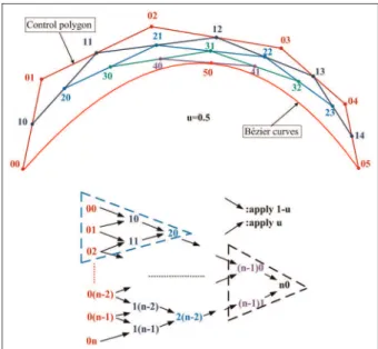
curves can be seen as a 12-dimensional nonuniform B-spline curve. Figure 1 shows a common method of using the triple NURBS curves to describe the cutter motion trajectory in five-axis machining.
In order to provide the CNC with complete cutter radius and length compensation information, an addi-tional third NURBS curve is used to describe the CC point’s vector. Compared with the traditional methods of cutter compensation vector description, it has the fol-lowing advantages:
1. Using the NURBS curve to describe the changes
of the CL point, the CA vector, and the CC point vector, the cutter processing path can be described more accurately and smoothly. Then, the final machining accuracy can be improved by ensuring the accuracy of the processing data.
2. Compared with the traditional method of the
five-axis space cutter compensation data
description, the triple NURBS curve has more accurate data information and a smaller amount of data input.
3. The triple NURBS interpolation method can
effectively combine with the RTCP technology, thus developing a highly precise and efficient NURBS interpolation method, which is com-plete and suitable for multi-axis processing.
4. The NURBS curve is continuously
differenti-able within the knots, so is the curve of the off-set CL point within the knots, which means that the cutter motion trajectory is also a smooth NURBS curve.
5. The motion curve of the offset CL point is
smooth and continuous, without the need to take into consideration the transition between seg-ments in traditional space cutter compensation.
Discretization of triple NURBS curves
In order to achieve high-precision interpolation of the triple NURBS curve and rapid equal error discretiza-tion of the NURBS curve, this article first decomposes the NURBS curve into three piece-wise rational Be´zier curve representation and then conducts the discretiza-tion of the piece-wise Be´zier curves. As the triple NURBS curve can be treated as a 12-dimensional B-spline curve, it only needs to compute the piece-wise Be´zier curve representation of the 12-dimensional B-spline curve. De Casteljau algorithm is employed in the discrete process.9 To simplify the discrete process and increase the universality of the algorithm, this article adopts the method of discretization of Be´zier curve at the parameter midpoint. In other words, for each Be´zier curve with standard parameter, if it cannot com-ply with the requirement of discrete error, the curve will
be subdivided at parameter point u= 0.5 to produce
two new Be´zier curves with standard parameter, until the precision requirement is met. Figure 2 shows the general process of De Casteljau algorithm. It can be observed that the discretization of Be´zier curve becomes the process of continuously generating control polygons which are closer to the curve using midpoint segmenta-tion algorithm.
Because the discrete process is carried out in the four-dimensional Euclidean space of the triple NURBS curve, the chord error for checking the discrete accuracy is defined in the three-dimensional space. Therefore, the discretization of the triple piece-wise rational Be´zier curve should obey the following principles:
1. The discrete accuracy of the triple NURBS
curve is determined by the accuracy requirement of C3(u). It has nothing to do with C1(u) and
C2(u). When checking precision, we only need
to check the accuracy of the rational Be´zier
curve determined byC3(u), that is, the accuracy
of the rational Be´zier curve determined by the CC point trajectory;
2. When checking the discrete accuracy of the
piece-wise rational Be´zier curve determined by the CC point trajectory, we need to project Be´zier points in the three-dimensional space and check them in accordance with the requirement of trajectory error in real-world processing;
3. The discrete processes of three piece-wise
rational Be´zier curves are synchronized. When the requirement of discrete accuracy ofC3(u) is
met and discretization ends, the discretization
of the two curvesC1(u) andC2(u) is terminated.
Hence, the discretization of the triple piece-wise rational Be´zier curve can be treated as that of a 12-dimensional Be´zier curve.
To further simplify the algorithm and increase com-puting accuracy, the termination condition of the seg-mentation of the Be´zier curve is defined as follows: the distance of Be´zier points corresponding to each Be´zier curve segment from both ending points of the segment should be smaller than the set control precision. It can be concluded using the convex hull of Be´zier curve that using this condition, the chord error of the Be´zier curve after discretization is smaller than required in the given control accuracy.
Description of space cutter compensation
Description of the data information of five-axis space
cutter compensation
In the five-axis motion control system with RTCP func-tion, since the control system can automatically trans-form the cutter position and orientation intrans-formation under the workpiece coordinate system into the motion volume of each axis in machine under the machine coordinate system, the calculation of five-axis space cutter compensation in such systems is carried out under the workpiece coordinate system. Therefore, the calculation of five-axis space cutter compensation only needs to recalculate the CL point position based on the CC point vector and current cutter parameter under the workpiece coordinate system.10
The length compensation of space cutter is an offset with the distance of Dlalong the CA vector!T. Hence, the vector of space cutter compensation can be obtained by computing the vector of cutter radius compensation.
As shown in Figure 3, !N is the surface unit normal vector of CC point, while!S is the surface unit tangen-tial vector of CC point along the feed direction. Assuming M!=!S 3!N, (!S,!M,!N) represents the local coordinate system of surface at CC point.11
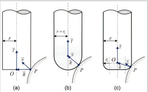
Similar to the three-axis milling, three types of cutter are usually used when processing surfaces with the
five-axis CNC machine. As shown in Figure 4, r and r1
denote the cutter radius and edge radius, respectively. Figure 4(a) shows the flat-end cutter with r1=0;
Figure 4(b) is the ball-end cutter with r=r1; Figure
4(c) is the fillet-end cutter withr.r1.0. Thus, it can be
seen that the flat-end and ball-end cutters are the spe-cial cases of fillet-end cutter. In order to fulfill the space cutter compensation function in an easier way, the edge center of fillet-end cutter, the bottom center of flat-end cutter, and the spherical centerOof ball-end cutter are defined as their respective cutter centers.
In addition, to better illustrate the relationship between CL point and CC point, as shown in Figure 5,
assuming that the CC point is denoted by P and the
CL point byO, then PO! is the vector of cutter radius compensation, referred to as!R. The normal vector of CC point is denoted by!N, CA vector by!T, and cutter length byl. The vector!V represents the unit vector on the same plane as!N and!T and is perpendicular to!T. It can be written as follows
V !
=
N !
!N !T!T
N !
!N !T!T
ð4Þ
Since the flat-end and ball-end cutters are the special cases of fillet-end cutter, we just need to analyze the latter one. As shown in Figure 4(c),Ois the result of offsetting ofPwith the distance ofr1alongN
!
first, then offsetting with a length ofralong!V, which can be expressed as
Figure 4. Types of five-axis milling cutter: (a) flat-end cutter, (b) ball-end cutter, and (c) fillet-end cutter.
R !
=ðrr1Þ
N !
!N !T!T
N !
!N !T!T
+r1N
!
=ðrr1ÞV
!
+r1N
!
ð5Þ
Cutter radius compensation without corner transition
A CC point trajectoryPaPb
!
is designated in the machin-ing program; the CA vectors at the startmachin-ing and endmachin-ing points are referred to asTa
!
andTb
!
, respectively; the unit normal vectors of surface at the starting and ending points are denoted byNa
!
andNb
!
, respectively.
Ball-end cutter. If N!a =N!b, then the CL point trajec-tory after compensation is OaOb
!
, which is offset by
PaPb
!
along the direction of !R with the distance ofr1,
while if Na
! 6¼Nb
!
, then the trajectory is a cylindrical spiral line as illustrated in Figure 5. For any point Pk
!
through interpolation, its CL point vector is Ok
!
. Hence, the formula ofOa
!
,Ob
!
,Ok
!
is as follows
Oi
!=P
i
!
+Ri
!
=Pi
!
+r1Ni
!
, i=a,b,k ð6Þ
Flat-end and fillet-end cutters. As the contact parts between flat-end and fillet-end cutters and the work-piece are constant, the relative relationship between CC point and the compensated CL point is also fixed. If
Na
!= N
b
! and T
a
!
=Tb
!
, the CL point path is a space line segments paralleling toPaPb
!
, while ifNa
! 6¼Nb
!
or
Ta
! 6¼Tb
!
, then the CL point Oa
!
,Ob
!
,Ok
!
based on the radius compensation formula is shown in equation (5).
Cutter radius compensation with corner transition
If there is a corner in the workpiece, the starting point vector of the trajectory before the corner is denoted as (P!1a,T!1a), surface normal vector as N!1a, the ending cutter point vector as (P!n,T!1b), surface normal vector as N1b
!
, the starting cutter point vector after the corner as (Pn
!
,T2a
!
), surface normal vector as N2a
!
, the ending cutter point vector as (P2b
!
,T2b
!
), and surface normal vector as N2b
!
. Pn
!
stands for the corner point; P1
!
(t) and P2
!
(t) for the CC point trajectory before and after the corner, respectively; and S1
!
and S2
!
for unit direc-tion vectors ofP!1(t) andP!2(t), respectively.
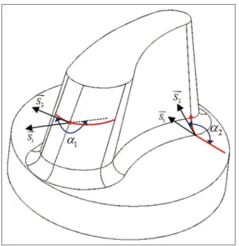
Let a be the processing side degree of the angle of
intersection between the CC point trajectoryP1
!
(t) and
P2
!(t). As illustrated in Figure 6, corners can be defined into two types based on the value range:
1. Outer corner (p\a1\2p);
2. Inner corner (0\a2\p).
Transitional processing of the outer corner. Assume that
O1
!(
t) andO2
!
(t) stand for the CL point trajectory after radius compensation. The ending points of O1
!
(t) and
O2 !(
t) areO1b
!
andO2b
!
, respectively. The compensation vectors from Pn
!
to O1b
!
and O2b
!
are R1b
!
and R2b
!
, respectively.
Ball-end cutter. As can be seen from Figure 7, the tra-jectory of the CL point after compensation is a circular arc withO1b
!
andO2a
!
as the starting and ending points, respectively; P!n as its center; andr1as radius.
Flat-end cutter and fillet-end cutters. IfTn
!
=T1a
!
=T2b
!
and the normal vector of the curved surface changes,
Pn
!, O
1b
!, andO
2a
!coexist in the flat-end cutter bottom plane, as bothR1b
!
andR2a
!
lie in this plane perpendicu-lar toTn
!
. Inserting a line segment betweenO1b
!
andO2a
!
will achieve transition of the corner and not cause over cutting to Pn
!
. While if the direction vector of the CA at the corner varies, the processing method is the same as the one applied in dealing with ball-end cutter.
Transitional processing of the inner corner
Ball-end cutter. As depicted in Figure 8, dashed lines are to show that the interference the cutter position has with P2
!
(t). The CL point is moved from O1b
!
to On
!
along the vertical direction until the distance from On
!
to P2
!
(t) reachesr. The return path pointsP01b
!
and P02a
!
are obtained by back calculatingOn
!
based on the com-pensation relation of R1b
!
and R2a
!
, respectively. Making P01b
!
the ending point of P1
!
(t) and P02a
!
the starting point ofP2
!
(t) forms two new CC point trajec-tories P01
!
(t) and P02
!
(t), and the radius compensation is made according to the new CC point trajectory. The formulas ofP01b
!
andP02a
!
are as follows
P01i
!
=On
! R1i
!
, i=a,b
On
!=O
1b
!+r 1
ffiffiffiffiffiffiffiffiffiffiffiffiffiffiffiffiffiffiffiffiffiffiffiffiffiffiffiffiffiffiffiffi
1N!1bS!2
2
r !
N1b
! N
1b
!S
2
!
S2
!
N1b
! N
1b
!S
2 ! S2 !
ð7Þ
Flat-end cutter. In the two circumstances illustrated in the left side of Figure 9, when the cutter is moving to
O1b
!, the interference with P
2
!(t) will not happen on condition that
T1b
!
S1
!
T1b
!
S2
!
.0 ð8Þ
P2
!(t). In this article, the interference is avoided through axial shifting, which means moving the CL point fromO1b
!
toOn
!
along the CA and making radius compensation according to the new CC points P01
!
(t) and P02
!
(t)
On
!=O
1b
!+ r T1b
!S
2
!
ffiffiffiffiffiffiffiffiffiffiffiffiffiffiffiffiffiffiffiffiffiffiffiffiffiffiffiffiffiffiffiffi 1 T1
b
!S
2
!
2
r T1b
!
ð9Þ
Fillet-end cutter. While processing the interference of fillet-end cutter, the traveling distance along the CA is the superposition of ball-end and flat-end cutters. The CAM system generates the initial triple NURBS machining program for the initial cutter according to the above process, while the space cutter compensation in CNC system is based on this initial program. Since the tool path and dealing with anti-interference of the compensated program are the same as the initial one, this compensation method is applicable to the tool whose radius and length change vary slightly from those of the initial cutter, for example, the radius change caused by cutter abrasion, the length change generated by cutter mounting, and so on.
Experiment and discussion
To validate the proposed method of using triple
NURBS curve to illustrate five-axis processing
Figure 6. Types of the corners.
Figure 7. Outer corner transition of ball-end cutter.
Figure 8. Transitional processing of the inner corner with ball-end cutter.
trajectory, surface data extracted from the blade model was used. Triple NURBS curve special for blade pro-cessing was generated through certain CAM approach as shown in Figure 10(a) and (b). All axis motion data fitting the two-turntable five-axis machine were pro-duced using the rapid discretization method mentioned in this article and the common RTCP algorithm.
In order to reduce machining error, this experiment used the easy cutting nylon bar, whose mechanical
property is stable. The workpiece surface after machin-ing was closer to the theoretical value. Durmachin-ing the experiment, initial data were generated using ball-end cutters, 4 mm in radius, at the feeding rate of 3000 mm/ min and with feed rate of 1 mm/r. When the 5-mm cut-ter was used for replacement during the process, the initial date could be modified according to space cutter compensation method mentioned in this article (per-missible error: 60.01 mm), and the modified data were used for processing.
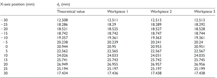
In order to verify the method, three workpieces were machined and measured in turn. The measurement method was as follows: without dismantling the work-piece after it was machined, the upper surface was made parallel to the X–Y plane while the Z, A, and C axes were fixed. Record the Y-axis coordinate value of the points, which were starting from the origin point of X-axis and extending to the positive and negative direc-tions at 5-mm intervals (Figure 10(c) and (d)), on both sides of the workpiece with the online measurement probe and make subtraction calculation (dy). The dia-meter of the ruby probe is 4 mm. According to the mea-surement data shown in Table 1, the actual values were within the permissible error range. Hence, the method put forward in this article that the cutter compensation along with RTCP could correctly express the complete processing path was verified.
Conclusion
This article focuses on the study of space cutter com-pensation technology of five-axis machine and pro-poses the triple NURBS curve path description method fitting the five-axis processing. With this method, the cutter position and orientation and CC point location during processing can be described more comprehen-sively, thereby achieving effective five-axis space cutter compensations. It can be observed from the experiment
Figure 10. The CAD model and experiment process: (a) CAD model, (b) CAM data processing, (c) machining and measurement, and (d) measuring method and positions.
Table 1. Y-axis coordinate difference value of the two points.
X-axis position (mm) dy(mm)
Theoretical value Workpiece 1 Workpiece 2 Workpiece 3
230 12.508 12.511 12.513 12.513
225 18.286 18.29 18.289 18.292
220 18.521 18.525 18.527 18.528 215 18.742 18.742 18.747 18.744 210 19.357 19.361 19.363 19.361
25 20.238 20.239 20.241 20.24
0 20.944 20.95 20.953 20.951
5 22.562 22.565 22.567 22.567
10 24.026 24.033 24.031 24.035
15 25.741 25.743 25.742 25.745
20 26.949 26.955 26.957 26.956
25 25.194 25.197 25.197 25.199
that the method can solve the space cutter compensa-tion problem in five-axis processing efficiently, thereby qualifying as a genuine five-axis NURBS interpolation method. In so doing, the capability of five-axis machines processing complex surface can be upgraded dramatically. Meanwhile, this method can also be applied to the space cutter compensation of other machines with multiple-axis structures, as the space cuter compensation function is realized in the work-piece coordinate system.
Declaration of conflicting interests
The authors declare that there is no conflict of interest.
Funding
This research was sponsored by the National Natural Science Foundation of China (nos 51475324 and 51105269), the National Key Technology R&D Program (no. 2013BAF06 B00), and Tianjin Science and Technology Plan Projects (nos 13JCZDJC34000 and 14JCZDJC39600).
References
1. Han L, Gao XS and Li H. Space cutter radius compensa-tion method for free form surface end milling.Int J Adv Manuf Tech2013; 67: 2563–2575.
2. Tung C and Tso PL. A generalized cutting location expression and postprocessors for multi-axis machine
centers with tool compensation. Int J Adv Manuf Tech
2010; 50: 1113–1123.
3. Liang SR and Lin AC. Probe-radius compensation for 3D data points in reverse engineering.Comput Ind2002; 48: 241–251.
4. Moreton DN and Durnford R. Three-dimensional tool compensation for a three-axis turning centre. Int J Adv Manuf Tech1999; 15: 649–654.
5. Chen YD, Wei HX and Wang TM. Three-dimensional tool radius compensation for a 5-axis peripheral milling. Adv Sci Lett2011; 4: 3093–3096.
6. Qiao Z, Wang T, Wang Y, et al. Be´zier polygons for the linearization of dual NURBS curve in five-axis
sculp-tured surface machining. Int J Mach Tool Manu 2012;
53: 107–117.
7. Yin S, Yu TT and Liu P. Free vibration analyses of FGM thin plates by isogeometric analysis based on clas-sical plate theory and phyclas-sical neutral surface.Adv Mech Eng2013; 2013: 634584.
8. Piegl L and Tiller W.The NURBS book. Berlin, Heidel-berg: Springer-Verlag, 2003.
9. Romani L and Sabin MA. The conversion matrix between uniform B-spline and Be´zier representations. Comput Aided Geom D2004; 21: 549–560.
10. Liu Z, Song X, Zhao Y, et al. Stiffness identification of spindle-toolholder joint based on finite difference
tech-nique and residual compensation theory.Adv Mech Eng
2013; 2013: 753631.
11. Lo CC. Real-time generation and control of cutter path
for 5-axis CNC machining.Int J Mach Tool Manu1999;