Theoretical Determination of Temperature Field in
Orthogonal Machining
Ojolo S. Joshua, Ismail S. Oluwarotimi
*, Yusuf O. Tolu
Department of Mechanical Engineering, University of Lagos, Lagos, Nigeria.
Received 07 June 2013; received in revised form 17 July 2013; accepted 20 August 2013
Abstract
In this work, mathematical models were developed to simulate the thermal behaviour of a cutting tool insert in three-dimensional dry machining. Models to determine the temperature rise at the shear plane and tool insert in orthogonal cutting were developed, simulated and validated. The effects of various machining parameters/variables such as specific heat of material of 4400J/kg, Depth of cut (t) of 0.0003m, Density of 7870kg/m3, Width of cut (b) of 0.005m, Chip thickness ratio (rt) of 0.42, Tool rake angle of 100, Cutting Velocity (V) of 35m/min and Shear force (Fs) of 1257.6N on temperature rise were well analyzed.
Keywords: temperature, machining variables, orthogonal machining
1.
Introduction
In orthogonal cutting, the cutting edge of the tool is perpendicular to the cutting speed direction. During the cutting, the work material ahead of the tool suffers plastic deformation and, after sliding on the rake face of the tool, goes to form the chip. The deformation process is highly concentrated in a very small zone and the temperatures generated in the deformation zones affect both the tool and the work piece (Portda, 2003). also the high cutting temperatures strongly influence tool wear, tool life, work piece surface integrity, chip formation mechanism and contribute to the thermal deformation of the cutting tool, which is considered, amongst others, as the largest source of error in the machining process, the increase in the temperature of the work piece material (mild steel) in the primary deformation zone softens the material, thereby decreasing cutting forces and the energy required to cause further shear.
Temperature at the tool-chip interface affects the contact phenomena by changing the friction conditions, which in turn affects the shape and location of both of the primary and secondary deformation zones, maximum temperature location, heat partition and the diffusion of the tool material into the chip (chiou, 2002). One of the most common operations in manufacturing is metal cutting. It is a quite complex phenomenon, of multi physics type, where elasticity and plasticity, fracture, contacts, heat transfer, among others takes place simultaneously. The purpose of a machining process is to generate a surface having a specified shape and acceptable surface finish, and to prevent tool wear and thermal damage that leads to geometric inaccuracy of the finished part.
The experimental measurement of the temperature and heat distribution in metal cutting is extremely difficult due to a narrow shear band, chip obstacles, and the nature of the contact phenomena where the two bodies, tool and chip, are in continuous contact and moving with respect to each other (Vernaza-Pena, 2002, Sutter et al, 2003). Therefore, analytical development of cutting temperature distribution can aid in addressing important metal cutting issues such as tool life and
* Corresponding author. E-mail address: smailrotimi@gmail.com
dimensional tolerance under practical operating conditions. Hence, as the objective of this study, mathematical models to determine the temperature fields in orthogonal machining were developed, simulated and validated using the existing data.
2.
Materials and Methods
2.1. Mathematical Models Develo (Modeling of Temperature Distribution in Tool Insert)
The tool insert has three plane boundaries in contact with the tool holder at x = a, y = b, and z = c. These boundaries will be assumed to be at the ambient interface, the temperature at the bottom surface of the insert (z = c) could be as high as 2000C under a different set of condition. So in this work, two types of thermal boundary conditions on ambient temperature and insulated surfaces considered. The three-dimensional transient heat conduction equation is
t T z
T y
T x
T
T
1
2 2 2 2 2 2
(1)
where
T is the thermal diffusivity of the material (mild steel). The initial condition is
x y z
TT , , ,0
The boundary conditions for the model without heat pipe are the following
a(i) The heat source is considered as a plane heat source on the top face of the insert with the following expression.
otherwise T
T h
L y L x for q t
z y x z T
k z c x y
0 , 0 ,
,
, 0
where qc is the heat flux flowing into the tool insert
a(ii) The adiabatic boundary conditions are assumed for the two surfaces which are close to the heat source (x = 0, y = 0) and the bottom surface (z =c) are the following
0, ,0 ,
0
x t c z y T
,0,0 ,
0
y t c z x T
0 ,
,
,
c z
z t z y x T
a(iii) The ambient boundary conditions are assumed for the two surfaces which are far away from the heat source (x = a, y = b) can be described as:
a yzt
TT , , ,
x
b
z
t
T
T
,
,
,
The boundary conditions for the model with heat pipe installed are:
b(i) The adiabatic boundary conditions for the two surfaces which are close to the heat source (x, 0, y = 0), the bottom surface (z = c + q) and the surface of insert (x = a, 0 < y < b, 0 < z < c) which is far away from heat source:
0 , 0
, , 0
(
x t q c z y T
0 , 0
, 0 ,
(
0 , , , c q z z t z y x T 0 , 0 , 0 , ( x t c z b y a TThe ambient boundary conditions for the two surfaces of the heat pipe which are far away from the heat source (x, a, 0 < y < p, and y = p):
T(a,0 y p,c z q,t T
T
t
z
p
x
T
(
,
,
,
)
2.2. The Model
Finite difference scheme was developed to solve the temperature distribution in orthogonal cutting.
nk j i n k j i n k j i n k j i n k j i n k j i n k j i n k j
i F T
T T T T T T F
T 0 ,,
1 , , 1 , , , 1 , 1 , , , 1 , , 1 0 1 ,
, 16
(2)
The stability criteria is
. . 6 1
0 ie
F 6 1 2 x t t x 6 2
Using implicit crank –Nicolson finite difference scheme, gives:
n k j i n k j i n k j i n k j i n k j i n k j i n k j
i T T T T T T
T t x 1 , , 1 , , , 1 , , 1 , , , 1 , 1 , , 2 3
2
(3)
On the LHS, we have seven unknowns and on the RHS all the seven quantities are known. This is an implicit scheme which is convergent for all values of
t x 2 (4) (5)
Table 1 Input values of thermal simulation of temperature distribution on tool insert
Width 100mm
Length 200mm
Thickness 5mm
Thermal conductivity 120 W/m K
Density 7800kg/ms
Specific heat 343.3J/kgK
Initial temperature 298K
2.3. Modeling Temperature Distribution in Shear Plane Using the principle of volume constancy, we have
c
.
.
.
.
b
v
t
b
v
t
c cwhere t, b and v respectively denote the depth of cut, width of cut and cutting velocity. Similarly tc, bc and vc denote chip thickness, width of chip and chip velocity respectively. When b is comparable to t, there is significant side flow (or strain in the direction of the width b) and bc is greater than b. the side flow being more on the edges the resulting chip is not even rectangular in shape. However, when b >> t, the side flow is negligible and we may take b equal to bc. In most cutting process b is nearly equal to bc. Hence,
c
v t v
t. 1
L L v v t
t
r c c
c
t
t
r
is the chip thickess ratio andL
1in the length of the chip formed from a layer of uncut chip of length L on the work
surface. From the geometry of Fig. 2 below, we can write the length of shear plane AC as
cos sin
c
t t
AC
where
is the rake angle of the tool. Hence,
cos sin
t c
r t
t
(6)
sin 1
cos
sin 1
cos tan
L L L L
r r
c c
t t
sin cos tan
c c
L L
L
(7)
sin cos tan
sin cos tan
1
t t
t or
L L
L
c c c
From Fig. 3 below,
Fh = horizontal force component parallel to the cutting velocity vector Fv = Vertical force component normal to Fv
Fs = Force component parallel to the shear plane Fp = Force component normal to Fs
If
is the average co-efficient of friction the interface between the chip and the tool, then,
t n
F F
and are related asfollows,
. .
tan
h t
F F
h
F Fv
tan
Also,
] Rcos
Fh andFs Rcos
where R is the resultant cutting force. But
sin
.k tbk
b AC
Fs
sin cos
0
bk t
R
cos
sin
k
b
t
R
(8)
cos
sin
cos
k
b
t
F
h (9)where k is the yield stress of the material in shear and is the friction angle. Velocity relationship in orthogonal cutting is shown in the Fig. 3 below. Applying the principle of triangle to the below triangle in Fig. 3 gives
sin 90
sin 90 sin
c
s V
V V
(10)
(a) as a three-dimensional process (b) showing shear zone rather than shear plane
Fig. 1 Orthogonal cutting
Fig. 2 Shear plane and shear plane angle
Fig. 3 Cutting force component in orthogonal machining
Fig. 4 Velocity relationship in orthogonal machining
2.4. Shear Plane Temparature in Orthogonal Cutting
The temperature rise at the shear plane can be approximately estimated by assuming a thin zone model of metal cutting and by assuming a uniform rise of temperature all over the shear plane. If Es be the energy per unit volume dissipitated at the shear plane, then;
MCw
q
, q MCw
s
i
, q wVCw
S
i
Introducing
which is the factor representing the fraction of heat retained by the chip.
s i
w
wC
V
q
s i
w w
C
E
w w i s C E
(11)Introducing
J
which is the heat equivalent of mechanical energyw w i s C J E
i w w s sC
J
E
V t b V FE s s
s
cos cos VVS (12)
Pe ES 664 . 0 1 1 (13) s
st ec
V Pe
4 cos
cos sin cos s E
] 1 [ cos sin cos 1 1 664 . 0 Pe
cos
sin
cos
cos
sin
664
.
0
1
1
Pe
cos cos sin 664 . 0 cos sin cos sin Pe PeSubstituting for
Pe
Substituting for
V
s where
cos cos V Vs
cos cos sin 664 . 0 cos sin cos cos 4 . cos 4 cos / cos sin cos . . cos ec V ec t V s S
cos 4 cos sin 66 . 2 sin cos cos sin cos . . cos s s ec V ec t V (14) i w w S S C E
w w
s i s C E
Substituting for Es
tV b C V F w w s s
s i
Also substituting for Vs
J C
bt F v t b C J FV w w s w ws i
cos cos cos cos
cos 4 cos sin 66 . 2 cos cos cos2 s s w w s Vt b C J V F Where tan1 cos 1 sin t t r r (15)
The parameters used to simulate the model are in Table 2 below
Table 2 Input Values of thermal simulation of temperature rise at the shear zone
Specific heat of material 4400J/kg
Density 7870kg/m3
Depth of cut (t) 0.0003m
Width of cut (b) 0.005m
Chip thickness ratio (rt) 0.42
Tool rake angle 100
Cutting Velocity (V) 35m/min Shear force (Fs) 1257.6N
3.
Results and Discussions
3.1. Results on Temperature Distribution on the Tool Insert
The tool insert was modeled using a finite element approach to study the temperature distribution behavior of a tool insert in machining. The material properties and dimension of the tool insert are shown in Table 2. The cases of the heat fluxes qc with 9.75×10⁶ W/m2, 8.125×10⁶ W/m2, 6.5×10⁶ W/m2, and 4.875×10⁶ W/m2 similar to those by previous researchers [2, 3] are used as the inputs to the cutting tool insert.
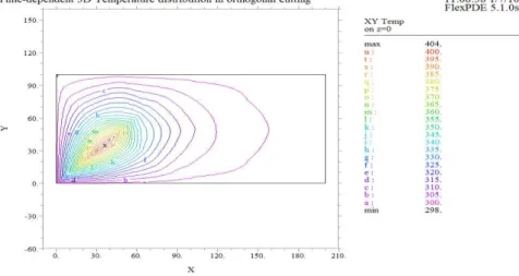
Data beside Fig. 4 shows the result generated by Chiou [4], it can be seen from their result that there is also a reduction in temperature farther from the tool tip and the maximum temperature occur at the tip. Their ambient condition is also 298K, while the maximum temperature is 386K. This validates the research study.
Fig. 5 shows the temperature distribution at the bottom surface of the tool insert, with the boundary conditions stated. The temperature distribution is evidently the same as the upper surface of the insert. This shows that at ambient conditions temperature distribution at the upper and lower surfaces of the tool insert are the same in continuous cutting. Fig. 6 shows temperature distribution on the tool insert when there is sufficient air cooling. It was shown that the temperature maintains a constant atmospheric condition.
It is noted that the air-cooled effects on the heat flux of both heat sources are rather minor. Thus, it can be suggested that the air cooled method does not alter the chip formation process. Furthermore, the simulation results of boundary conditions and coolants were done to see the effects on the cutting tool. It is noted that the Finite Element Analysis (FEA) shows that the cutting tip maintained a constant atmospheric temperature when the cutting tool is efficiently air-cooled but the temperature increases rapid when the tool is subjected to adiabatic boundary conditions without cooling. The simulated tool temperatures reasonably agree with the previous results [4, 5].
The models can be used to investigate the effects of the major parameters on the cooling efficiency. Without involving intensive computation for chip formation analysis, this study used the derived heat-source characteristics as the input of temperature simulations. FEA models can be used to study machining temperatures at external cooling conditions without complex chip formation analysis. Such an approach provides an efficient analysis, with reasonable accuracy, to evaluate cutting temperatures when external cooling is present. The current models require heat source input from machining tests.
Fig. 4 The Temperature Distribution against Distance on the Tool Insert
Fig. 6 The temperature distribution against time on the cutting tool when there an effective air-cooling on the cutting tool
Fig. 7 Effect of velocity on temperature rise at different rake angles
Fig. 8 Effect of force on temperature rise at different rake angles
Fig. 9 Effect of velocity on temperature rise Fig. 10 Effect of chip thickness on temperature rise
0 5 10 15 20 25 30 35 40
0 50 100 150 200 250 300 350 400
Velocity(m/min)
T
e
m
p
e
ra
tu
re
R
is
e
(
C)
Fs = 1000N Fs = 1333.3333N Fs = 1666.6667N Fs = 2000N
0.1 0.2 0.3 0.4 0.5 0.6 0.7 0.8 0.9 1 0
100 200 300 400 500 600 700
chip thickness (mm)
T
e
m
p
e
ra
tu
re
R
is
e
(
Fig. 11 Effect of thickness ratio on temperature rise
3.2. Results on Temperature Rise at the Shear Zone in Orthogonal Machining
The temperature rise at the shear plane is estimated by assuming a thin zone model of metal cutting. The shear plane is assumed as a moving source of a heat band on the work piece.
Fig. 7 above shows that the temperature increases with an increase of the cutting speed with different rake angles. The dependence of the temperature on the cutting speed is more pronounced for an increase from 0–10 m/min. For cutting speeds larger than 38 m/min, the temperature seems to stabilise at 2380C. Also, it can be noted that the higher the rake angle of cut the lower the temperature, but the different rake angles do not affect the velocity of cut. The relationship between cutting speeds and mean rake temperature measured using the so-called tool-work thermocouple method, when turning the titanium alloy was represented [6]. With decreasing feed rate, or increasing inclination angle, or both, the temperature decreases.
In addition, by increasing the inclination angle the chip curl radius and the chip contact length were reduced. The mean rake temperature was not affected by use of a coolant in continuous orthogonal turning. Also, the temperature increases with an increase of the cutting speed [7]. The dependence of the temperature on the cutting speed is more pronounced for an increase from 0–10 m/min. For cutting speeds larger than 38 m/min, the temperature seems to stabilize at 2380C. These two results validate the model shown in Fig. 6.
Fig. 8 shows that with an increase in shear force, there is a corresponding increase in temperature rise. This shows that a small increase in the shear force results in an increase in temperature irregardless of the point and there is no stability in temperature due to an increment in force. The cutting force decreases as the tool rake angle increases.
The tool rake angles have significant influence on the cutting temperature. Increase in rake angle will reduce temperature by reducing the cutting forces but too much increase in rake will raise the temperature again due to reduction in the wedge angle of the cutting edge. It is clear that the relationship between the tool rake angle and the cutting and feed forces is linear [8]. Also, he concluded that the cutting temperature increases with a decrease in the tool rake angle. Temperature measurements obtained during experimental runs were in agreement with recent work conducted [9, 10].
The result in Fig. 9 indicates an increase in velocity results in a decrease in shear force. This is due to the thermal softening effect over strain hardening effect as cutting speed increases. It is noticed that an increase in cutting velocity leads to a decrease of the force. The force decreases as the rake angle increases. as shown in Fig. 8 above, the cut was orthogonal with feed of 0.08mm/rev, depth of cut 2.55mm, and cutting speeds of 240, 600, 1000m/min with rake angle of -50.
0 0.1 0.2 0.3 0.4 0.5 0.6 0.7 0.8 0.9 1
230 240 250 260 270 280 290 300
Thickness Ratio
Te
m
pe
ra
tu
re
R
ise
(
The effect of thickness on temperature rise is presented in Fig. 10, it can be seen that the thinner the thickness, the higher the temperature rise. From Fourier law, we see that the rate of heat loss is inversely proportional to area. When thin cross section is taken compared with a thick cross section, it could be seen that there is a higher rate of temperature rise in the thin cross section compared to the thin cross section. Therefore, with the above reasoning, it could be concluded that temperature rises with reduction in thickness and reduces with reduction in thickness, this also validate the result generated in this model.
Thickness ratio against temperature rise is presented in Fig. 11, from 0-0.2, the temperature reduces, at 0.2, the temperature is at a minimum (2320C), from 0.2 thickness ratio above, we have a steady increase in temperature i.e. the dependence of temperature is on the thickness ratio is more pronounce at these points.
4.
Conclusions
The temperature of a tool plays an important role in thermal distortion and the machined part’s dimensional accuracy, as well as in tool life in machining. Therefore, in this work, an approach using the Finite Element Analysis (FEA) was developed to simulate the thermal behaviour of a carbide cutting tool in three-dimensional dry machining. The particular temperature distribution depends on density, specific heat, thermal conductivity, shape and contact of the tool. FEA shows that the cutting tip maintained a constant atmospheric temperature when the cutting tool is efficiently air-cooled but the temperature increases rapid when the tool is subjected to adiabatic boundary conditions.
Also, a model to determine the temperature rise at the shear plane was developed, and it was used to determine the effect of various parameters on temperature rise. Summarily, the finite element model shows the temperature distribution on the tool insert with dimensions 100mm by 200mm at the point of maximum temperature of 404K. From the result, the maximum temperature does not occur at the tool tip, because part of the temperature has been convected away as a result of the cutting fluid but it occurs very close to the cutting tip, while the minimum temperature apart from the ambient condition (298K) occur at the extreme of the tool insert. The dependence of the temperature on the cutting speed is more pronounced for an increase from 0–10 m/min. For cutting speeds larger than 38 m/min, the temperature seems to stabilise at 2380C.
References
[1] J. C. Jaeger, “Moving sources of heat and the temperatures at sliding contacts, ” Proceedings Royal Society of NSW, Aug. 1942, pp. 203–224.
[2] R. Radulescu and S. G. Kapoor, “An analytical model for prediction of tool temperature fields during continuous and interrupted cutting,” Transactions of the ASME, Journal of Engineering for Industry, vol. 116, pp. 135-143, 1994. [3] A. O. Tay, M. G. Stevenson and G. De Vahl Davis, “Using the finite element method to determine temperature
distributions in orthogonal machining,” Proceedings of the Institution of Mechanical Engineers, pp. 627–638, Mar. 1974. [4] R. Y. Chiou, J. S. Chen, Lin Lu, and Ian Cole, “Prediction of heat transfer behavior of carbide insert with embedded heat
pipes for dry machining,” Proceedings of IMECE, 2002.
[5] A. O. Bareggi, G. E. Donnell, and A. Torrance, “Modelling thermal effects in machining by finite element methods,’’ Proceedings of the 24th International Manufacturing Conference, Waterfall, vol. 1, pp. 263-272, Aug. 2007.
[6] T. Kitagawa, A. Kubo, K. Maekawa, “Temperature and wear cutting tools in high-speed machining of Inconel 718 and Ti-6Al-6V-2Sn,” Wear 202, pp. 142–148, 1997.
[7] G. Sutter, L. Faure, A. Molinari, N. Ranc and V. Pina, “An experimental technique for the measurement of temperature
fields for the orthogonal cutting in high speed,” International Journal of Machines Tools and Manufacture, vol. 43, pp.
671–678, 2003.
[8] M. C. Shaw, “Some observations concerning the mechanics of cutting and grinding,” Applied Mechanics, Rev. 46, pp. 74-79, 1993.
[9] K. M. Vernaza-Pena, J. J. Mason, M. Li, “Experimental study of the temperature field generated during orthogonal
machining of an aluminium alloy,” Experimental Mechanics, vol. 42, pp. 222–229, 2002.
[10] H. Y. K. Potdar and A. T. Zehnder, “Measurements and simulations of temperature and deformation fields in transient