Sparse Spatial Coding: a novel approach for efficient and accurate object recognition

SPARSE SPATIAL CODING:

A NOVEL APPROACH FOR EFFICIENT AND

GABRIEL LEIVAS OLIVEIRA

SPARSE SPATIAL CODING:

A NOVEL APPROACH FOR EFFICIENT AND

ACCURATE OBJECT RECOGNITION

Dissertação apresentada ao Programa de Pós-Graduação em Ciência da Com-putação do Instituto de Ciências Exatas da Universidade Federal de Minas Gerais como requisito parcial para a obtenção do grau de Mestre em Ciência da Com-putação.

O

: M

C

GABRIEL LEIVAS OLIVEIRA

SPARSE SPATIAL CODING:

A NOVEL APPROACH FOR EFFICIENT AND

ACCURATE OBJECT RECOGNITION

Dissertation presented to the Graduate Program in Ciência da Computação of the Universidade Federal de Minas Gerais in partial fulfillment of the requirements for the degree of Master in Ciência da Com-putação.

A

: M

C

c

2012, Gabriel Leivas Oliveira. Todos os direitos reservados.

Oliveira, Gabriel Leivas

D1234p Sparse Spatial Coding: A Novel Approach for Efficient and Accurate Object Recognition / Gabriel Leivas Oliveira. — Belo Horizonte, 2012

xv, 63 f. : il. ; 29cm

Dissertação (mestrado) — Universidade Federal de Minas Gerais

Orientador: Mario Campos

1. Sparse coding. 2. Object recognition. I. Título.

[Folha de Aprovação]

ela deve ser digitalizada e armazenada no disco em formato gráfico.

Se você estiver usando o♣❞❢❧❛t❡①,

armazene o arquivo preferencialmente em formato PNG (o formato JPEG é pior neste caso).

Se você estiver usando o❧❛t❡①(não o♣❞❢❧❛t❡①), terá que converter o arquivo gráfico para o formato EPS.

Em seguida, acrescente a opção❛♣♣r♦✈❛❧❂④nome do arquivo⑥

We are what we repeatedly do. Excellence then, is not an act, but a habit. Aristotle

❆❝❦♥♦✇❧❡❞❣♠❡♥ts

First and foremost I would like to thank my advisor. Prof. Mario Campos is a great advisor, who was always supportive in my research endeavors and has taught me a lot about robotics, computer vision, and research in general.

I also need to thank all the people at VeRLab, Elizabeth, Samuel, Yuri, Ar-mando, Douglas and Wolmar for the great interaction during this journey. Specially, I need to thank Erickson to introduce me to compressive sensing and for help me during this journey and Antônio Wilson for the partnership in several projects and for the close help with my dissertation.

The last, but not the least persons that I owe to thanks are my parents, my brother and my girlfriend for the unconditional support and to always give me strength to hunt my goals.

Thank all that make my masters at UFMG so enriching and unique experi-ence!

❘❡s✉♠♦

Até recentemente o reconhecimento de objetos, um problema clássico da Visão Com-putacional, vinha sendo abordado por técnicas baseadas em quantização vetorial. Entretanto, atualmente, abordagens que utilizam representação esparsa tem ap-resentado resultados significativamente superiores às técnicas usuais. Entretanto, uma desvantagem de métodos baseados em representação esparsa é o fato de car-acterísticas similares poderem ser quantizadas por conjuntos diferentes de palavras visuais.

Esta dissertação apresenta um novo método de reconhecimento de objetos de-nominado SSC – Sparse Spatial Coding – o qual é caracterizado pelo aprendizado do dicionário utilizando representação esparsa e codificação baseada em restrição es-pacial. Dessa forma, minimiza-se significativamente o problema típico encontrado em representações estritamente esparsas.

A avaliação do SSC foi realizada por meio de experimentos aplicando-o às bases Caltech 101, Caltech 256, Corel 5000 e Corel 10000, criadas especificamente para avaliação de técnicas de reconhecimento de objetos. Os resultados obtidos demonstram desempenho superior aos reportados na literatura até o momento para os métodos que utilizam um único descritor. O método também superou, para as mesmas bases, vários outros métodos que utilizam múltiplas características, e apre-sentou desempenho equivalente ou apenas ligeiramente inferior a outras técnicas. Finalmente, para verificarmos a generalização, o SSC foi utilizado para o reconheci-mento de cenas nas bases Indoor 67, VPC e COLD tendo apresentado desempenho comparável ao de abordagens do estado da arte para as duas primeiras bases e su-perior na base COLD.

Palavras-chave: Visão computacional, Reconhecimento de objetos, Representação esparsa.

❆❜str❛❝t

Successful state-of-the-art object recognition techniques from images have been based on powerful techniques, such as sparse representation, in order to replace the also popular vector quantization approach. Recently, sparse coding, which is characterized by representing a signal in a sparse space, has raised the bar on sev-eral object recognition benchmarks. However, one serious drawback of sparse space based methods is that similar local features can be quantized into different visual words.

We present in this thesis a new object recognition approach, called Sparse Spa-tial Coding (SSC), which combines a sparse coding dictionary learning and a spaSpa-tial constraint coding stage. Thus, we minimize the problems of pure sparse represen-tations. Experimental evaluation was done at Caltech 101, Caltech 256, Corel 5000 and Corel 10000, that are datasets specifically designed to object recognition evalu-ation. The obtained results show that, to the best of our knowledge, our approach achieves accuracy beyond the best single feature method previously published on the databases. The method also outperformed, for the same bases, several methods that use multiple feature, and provide equivalent to or slightly lower results than other techniques. Finally, we verify our method generalization, applying the SSC to recognize scene in the Indoor 67 scene dataset, VPC and COLD, displaying perfor-mance comparable to state-of-the-art approaches in the first two bases and superior in COLD dataset.

Keywords: Computer Vision, Object recognition, Sparse coding.

▲✐st ♦❢ ❋✐❣✉r❡s

1.1 Graphical representation of a sparse vector . . . 2

1.2 This figure shows an input signalxthat is a linear combination of the dic-tionaryDand it activation vectorµ. Cells filled with blue color represent the active dictionary elements ofx. . . 3

1.3 Example of multi scale pooling, called spatial pyramid matching, by [Lazebnik et al., 2006]. . . 4

3.1 Object recognition system overview . . . 18

3.2 Sparse coding vs locality . . . 25

3.3 PCA vs OCL. . . 28

3.4 SVM 2 classes separation . . . 30

4.1 Performance of different sizes of dictionaries (Caltech 101) . . . 33

4.2 Performance of different number of neighbours (Caltech 101) . . . 34

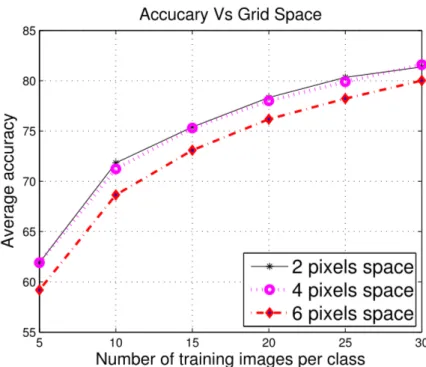
4.3 Performance of different number grid spaces (Caltech 101) . . . 35

4.4 Performance of different number grid sizes, i.e. 16, 24, and 32 pixels. . . 36

4.5 Number of Components analysis . . . 38

4.6 Epochs analysis . . . 39

4.7 Caltech 101 dataset class samples, for example chair, camera and head-phone in the first row and laptop, revolver and umbrella below them. . . 39

4.8 Caltech 256 dataset. These three pairs of classes (box glove, ipod and baseball bat) illustrate the high intra-class variance of Caltech 256. . . . 42

4.9 MIT 67 Indoor examples of image classes with high in-class variability and few distintive attributes (corridor class). . . 44

4.10 Average classification rates for MIT 67 indoor scene dataset . . . 44

4.11 Lighting conditions of COLD dataset. . . 47

4.12 Average results on COLD-Ljubljana dataset . . . 48

▲✐st ♦❢ ❚❛❜❧❡s

4.1 System variables gain . . . 35

4.2 Off-line methodologies comparison . . . 37

4.3 Online Learning Results . . . 38

4.4 Recognition results on Caltech 101 . . . 40

4.5 Our Method gain on Caltech 101 . . . 40

4.6 Recognition results on Caltech 101 (Multiple Features) . . . 41

4.7 Average accuracy on the Caltech 256 dataset . . . 42

4.8 Comparison of Caltech 256 results with a dictionary of 4096 basis. . . 42

4.9 Results in Corel datasets . . . 43

4.10 Statistical analysis Caltech 101 single feature . . . 46

4.11 Statistical analysis Caltech 101 multiple feature . . . 46

4.12 Statistical analysis Caltech 256 . . . 46

4.13 Statistical analysis in Corel datasets . . . 46

4.14 COLD recognition rates for equal illumination conditions . . . 48

4.15 COLD results . . . 49

4.16 Recognition rates from VPC dataset dataset . . . 50

A.1 Confidence Intervals Caltech 101 single feature . . . 61

A.2 Confidence Intervals Caltech 101 multiple feature . . . 61

A.3 Confidence Intervals Caltech 256 . . . 62

A.4 Confidence Intervals Corel datasets . . . 62

A.5 Confidence Interval MIT-67 Indoor datasets . . . 62

B.1 VPC P-Values . . . 63

▲✐st ♦❢ ❆❝r♦♥②♠s

SC Sparse Coding VQ Vector Quantization SPM Spatial Pyramid Matching BoF Bag-of-Features

SPAMS Sparse Modeling Library SSC Sparse Spatial Coding

PCA Principal Component Analysis SVM Support Vector Machine

OMCLP Online Multi-class LPBoost SVD Singular Value Decomposition CBIR Content-Based Image Retrieval OCL Orthogonal Class Learning

CRBM Convolutional Restricted Boltzmann Machine

❈♦♥t❡♥ts

Acknowledgments vii

Resumo viii

Abstract ix

List of Figures x

List of Tables xi

List of Acronyms xii

1 Introduction 1

1.1 Sparse representations . . . 2

1.2 Non-sparse representations . . . 2

1.2.1 Dictionary Learning . . . 3

1.2.2 Pooling . . . 4

1.3 Problem definition . . . 4

1.4 Publications . . . 6

1.5 Contributions of the Thesis . . . 7

1.6 Thesis Outline . . . 7

2 Related Works 8 2.1 Geometrical approaches . . . 9

2.1.1 Alignment algorithms . . . 9

2.1.2 Geometrical hashing methods . . . 10

2.2 Appearance based methods . . . 10

2.3 Feature Points Object Recognition . . . 11

2.3.1 Non-sparse methods . . . 12

2.3.2 Sparse representation methods . . . 13

2.4 Considerations . . . 15

3 Methodology 17 3.1 Feature Extraction . . . 17

3.1.1 SIFT Descriptor . . . 19

3.2 Unsupervised feature learning . . . 20

3.2.1 Dictionary Learning . . . 21

3.2.2 Solving Dictionary Learning . . . 22

3.3 Coding Process . . . 24

3.4 Pooling . . . 25

3.5 Off-line learning method . . . 27

3.6 Online learning method . . . 29

3.6.1 SVM . . . 29

4 Method Validation 31 4.1 Parameter Settings . . . 31

4.1.1 System Parameters Analysis . . . 32

4.1.2 Parameter Analysis conclusions . . . 34

4.2 Evaluation of Offline Methods . . . 36

4.3 Online Learning Evaluation . . . 37

4.4 Caltech 101 . . . 38

4.5 Caltech 256 . . . 41

4.6 Corel Datasets . . . 43

4.7 MIT 67 Indoor . . . 43

4.8 Statistical Analysis . . . 45

4.9 COLD Dataset . . . 47

4.10 VPC . . . 49

5 CONCLUSION 51 Bibliography 53 6 Attachments 60 A Confidence Interval Values 61 A.1 Confidence Intervals Caltech 101 . . . 61

A.1.1 Caltech 101 single feature . . . 61

A.1.2 Caltech 101 multiple feature . . . 61

A.2 Confidence Interval Caltech 256 . . . 61

A.3 Confidence Interval Corel Datasets . . . 62 A.4 Confidence Interval MIT-67 Indoor Datasets . . . 62

B VPC dataset P-values 63

❈❤❛♣t❡r ✶

■♥tr♦❞✉❝t✐♦♥

Recognizing objects in images has been a challenging task, and for a good number of years it has attracted the attention of a large number of researchers from sev-eral research communities such as robotics, computer vision and machine learning. Although almost all proposed techniques are based on good data representation, an inadequate representation can greatly influence the accuracy of those methods. Generally, these feature representations are designed manually or need significant prior knowledge. Therefore, to overcome this issue we present a novel coding pro-cess that automatically learns a representation from unlabeled data. Additionally, we explain how to build a sparse representation of an image, which represents an input signal, in our case data extracted from image patches, as a small combination of basis vectors, used to learn low level representations from unlabeled data.

Sparse Coding (SC) techniques are characterized by a class of algorithms that learn basis functions from unlabeled input data in order to capture high-level fea-tures. These high level features are signatures that encode an input signal as a com-bination of a small number of elementary signals. Frequently, those signals are se-lected from a dictionary. SC has been successfully used for image denoising [Elad and Aharon, 2006] and image restoration [Mairal et al., 2008b,a]. However, only recently SC has been effectively applied to replace Vector Quantization (VQ) tech-niques in object recognition tasks, and it is now considered the state-of-the-art with the best results for several datasets [Yang et al., 2009b; Jiang et al., 2011].

Before we fully state our problem, we will first introduce some key definitions used throughout this text, and more specifically in our methodology. These terms are: sparse and non-sparse representations, dictionary learning and pooling process.

1. INTRODUCTION 2

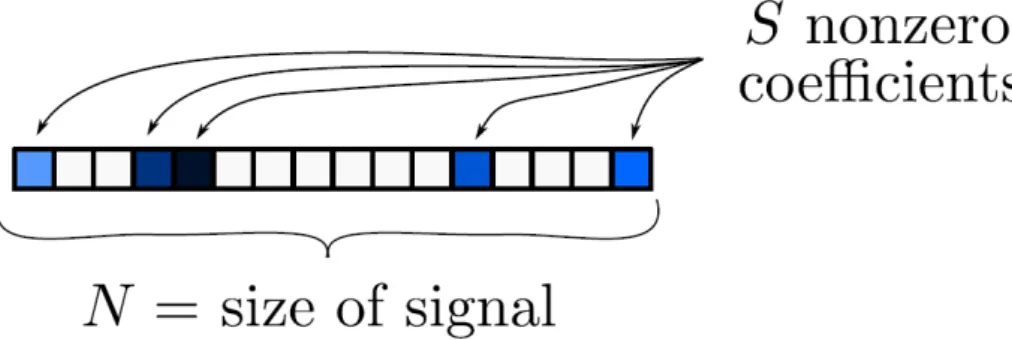
Figure 1.1: Graphical representation of a sparse vector. Srepresent the active coef-ficients for an input signal X. To be considered a sparse representation the number of activations must be a fraction of the total number of elements that could express such signal (S≪ N).

✶✳✶ ❙♣❛rs❡ r❡♣r❡s❡♥t❛t✐♦♥s

Let Xǫ Rn be a discrete signal. X is S-sparse if it is a linear combination of Sbasis vectors, whereS ≪ N. Figure 1.1 exemplifies a sparse vector.

Furthermore, it is worth to explain that this kind of representation assumes that the input signal is also sparse. Therefore, similarly to Yang et al. [2008], we employ image patches as our sparse input signal to perform object recognition. Our motivation to use sparse representations was based mainly on the following obser-vations:

• Sparse representation methods show robustness to signal recovery from noisy data;

• Sparsity has also been regarded as likely to be separable in high-dimensional sparse spaces [Ranzato et al., 2006] and therefore suitable for classification.

✶✳✷ ◆♦♥✲s♣❛rs❡ r❡♣r❡s❡♥t❛t✐♦♥s

Non-sparse representations can be seen as a signal composed by a set of values, where most of them are non-zero. For example, SIFT [Lowe, 2004] descriptors are composed by 128 float numbers, where the majority of them are not zero. Ap-proaches to recognition generally concatenate SIFT descriptors to obtain an image signature that can be considered non-sparse or dense.

1. INTRODUCTION 3

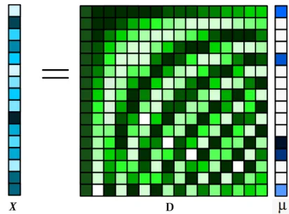
Figure 1.2: This figure shows an input signal x that is a linear combination of the dictionary D and it activation vector µ. Cells filled with blue color represent the active dictionary elements of x.

x2 =argminkxk₂s.t. Ax =ythat represent a sampleyas a linear combination

of training samplesA.

• sparse (l1 normalization), produce a sparse number of active coefficients.

x1 =argminkxk₂s.t. an approximation ofl0 normalization.

✶✳✷✳✶ ❉✐❝t✐♦♥❛r② ▲❡❛r♥✐♥❣

Dictionary learning algorithms receive as input tokens that, in our case, are random image patches, and learn P, which in this work will be generally considered to be

P=1024, basis functions.

For a set of input signalsx(1),x(2), ...,x(m) inRm×n, we learn a dictionary that is a collection of basesD₁,D₂, ...,D_k inRm×p, so that each inputxcan be decomposed as:

x=

m

∑

j=1

D_jµj, (1.1)

s.t.µ_j′_sare mostly zero,

whereµjis the set of basis weights for each input signal. Figure 1.2 depicts a

1. INTRODUCTION 4

Figure 1.3: Example of multi scale pooling, called spatial pyramid matching, by [Lazebnik et al., 2006].

✶✳✷✳✷ P♦♦❧✐♥❣

Pooling consists of summarizing the coded features across an image to form a global image representation. The objective of such method is to achieve invariance to im-age transformation and robustness to noise and clutter, removing spurious data while preserving relevant information.

Several pooling functions were proposed to build image signatures, and those that attained higher success were average and max pooling. Max pooling extracts the largest response in the collection of descriptors with respect to each dictionary element. We have chosen this function, in lieu of average pooling, since the works of Liu et al. [2011]; Boureau et al. [2010b] prove that max pooling attains state-of-the-art results. In addition, we perform max pooling in a spatial pyramid image representation, Figure 1.3. This is preferable, since max pooling under different locations and spatial scales provides more robustness to local transformations.

✶✳✸ Pr♦❜❧❡♠ ❞❡✜♥✐t✐♦♥

1. INTRODUCTION 5

an important component of state-of-the-art object recognition techniques [Boureau et al., 2010a; Gao et al., 2010; Wang et al., 2010; Yang et al., 2009b; Coates et al., 2011]. Indeed, using SPM is preferable to improve visual object recognition, since it creates geometrical relationships between features, which combined to SC, leads to high accuracy results.

This work presents a new approach, called Sparse Spatial Coding (SSC), for object recognition which takes advantage of SPM and overcomes SC drawbacks by implementing a spatial Euclidean coding representation.

Our method is composed of three main steps:

• Training phase;

• Coding phase;

• The use of an learning approach, that could be an off-line classifier, called Or-thogonal Class Learning (OCL), or an online method.

In the Training Phase the dictionary is built. Image patches are randomly ex-tracted from the set of training images, they are normalized and then are passed on to the learning process that builds the dictionary.

The Coding Phase can be divided into two steps: i) the extraction of local de-scriptors, which may use descriptors like SIFT [Lowe, 2004] or SURF [Bay et al., 2006], and ii) code generation, based on the dictionary and on the quantization of each descriptor, using a spatial constraint, instead of just sparsity. Next, the codes associated with each region are pooled together to form a global image signature.

The final stage of our method sends the global features to one of the two classi-fication methods. The first method is an off-line methodology called OCL that takes advantage of the high dimensionality of feature vectors when compared with the number of feature examples. The second possible classifier is an online classifica-tion method. We chose to use online learning motivated by requirements of tasks that need to be executed by mobile robots : i) small memory availability; ii) large amount of data, and iii) suitability for data streaming.

Online learning is well suited to several robotic tasks where, in general, the robot does not have access to the entire data domain. This is also very similar to decision making problems, where parts of the data are incrementally presented over time [Saffari et al., 2010]. This idea can be exemplified by a simple game quiz, with a student and a teacher executentimes the following steps:

1. INTRODUCTION 6

2. The student responds to the input with a prediction.

3. The teacher reveals the true answer for the input.

4. If the prediction is correct, then the model is reinforced, if it is wrong, the student is penalized and his model is updated.

The goal of the student is to minimize the cumulative error over time by up-dating its internal model of the problem.

Experimental results presented later in the work show that, to the best of our knowledge, the results we obtained over several object recognition datasets, such as Caltech 101, Caltech 256, Corel 5000 and Corel 10000, showing accuracies be-yond the best published results so far on the same databases. We also show that the proposed approach achieves state-of-the art performance on the COLD place recognition dataset.

In addition, high performance results were obtained on the MIT-67 indoor scene recognition dataset and VPC Visual Place Categorization dataset.

✶✳✹ P✉❜❧✐❝❛t✐♦♥s

Results from the work developed in this thesis were accepted for publication in two major conferences in the field, and another one will be submitted to IROS 2012:

Conferences and Workshops

• Oliveira, G. L. ; Nascimento, E. ; Vieira, A. W. ; Campos, M. . Sparse Spatial Coding: A Novel Approach for Efficient and Accurate Object Recognition In: 2012 IEEE International Conference on Robotics and Automation , 2012, St. Paul - Minnesota - USA.

QualisA1

1. INTRODUCTION 7

✶✳✺ ❈♦♥tr✐❜✉t✐♦♥s ♦❢ t❤❡ ❚❤❡s✐s

The main contributions of this thesis are:

• A novel unsupervised feature learning method which uses SC for dictionary learning and a coding stage based on spatial constraint, called Sparse Spatial Coding (SSC);

• An object recognition technique based on an online classification method, which when combined with the previous steps, leads to state-of-the-art per-formance results on several benchmark datasets;

• A new off-line method called OCL, which takes advantage of the high dimen-sionality of features when compared to the number of feature examples;

• A deep parameter analysis of the most relevant settings, showing their effects on system accuracy and performance.

✶✳✻ ❚❤❡s✐s ❖✉t❧✐♥❡

This thesis is structured as follows:

Chapter 2: We present and discuss related works on object recognition, focus-ing on sparse representation methods. Moreover, we give special attention to un-supervised feature learning methods that use sparse representation and additional constraints, like spatial similarity.

Chapter 3: Sparse Spatial Coding (SSC), which combines a sparse coding dic-tionary learning approach with a coding module which considers both sparsity and locality is carefully laid out in this chapter. We also present a novel off-line classifica-tion method, called Orthogonal Class Learning (OCL), that builds compact feature signatures to improve memory efficiency. In addition, we present an online learning algorithm that is a key part of our final object recognition approach.

Chapter 4: This chapter describes experimental results for a series of object recognition datasets namely, Caltech 101, Caltech 256, Corel 5000 and Corel 10000 and three scene/place recognition datasets, Indoor 67, VPC and COLD. Further-more, an empirical analysis is performed on the main system parameters, showing the effects of their settings to system performance.

❈❤❛♣t❡r ✷

❘❡❧❛t❡❞ ❲♦r❦s

One of the most fundamental problems dealt with by the computer vision commu-nity is object recognition, which is concerned with identifying which type of object or set of objects are presented in an image. Solving this problem accurately, and if possible with low computational burden, directly impacts several research areas, like robotics perception and content-based image retrieval.

Seminal works that address object recognition are dated more than four decades ago [Agin, 1972; Binford, 1971]. Some limited scope applications have achieved significant success such as: handwriting digits, human face and road signs recognition tasks. In the 70’s, as range sensors became popular, 3D data was read-ily available and used. In the 80’s, 2D images were commonly used, however ob-ject data were obtained under controlled conditions, with uniform background and structured lighting to facilitate the segmentation step. The first approaches dealt with a single object class under several viewpoints, and only later multi-class meth-ods appeared. Nonetheless, those techniques explored only a limited number of categories in controlled environments.

Object recognition methods can be divided into three main categories:

• Geometry based;

• Appearance based;

• Feature-points algorithms.

Many of the first object recognition techniques use geometrical representations based on edge contours extracted from object image. Those methods present some interesting features such as being almost unaffected by illumination changes and to variations in appearance due to different viewpoints.

2. RELATEDWORKS 9

Appearance based algorithms try to solve the object recognition problem by computing eigenvectors. While this kind of algorithms shows good results for object recognition tasks under significant viewpoint and illumination changes, they are affected by occlusion.

The last group of object recognition approaches are characterized by finding feature points, often present at intensity discontinuity on images. Although feature based algorithms present robustness to clutter scenes and partially occluded objects, they fail for textureless images and to small number of extracted keypoints.

✷✳✶ ●❡♦♠❡tr✐❝❛❧ ❛♣♣r♦❛❝❤❡s

The first efforts to tackle the object recognition problem used data produced by range sensors [Agin, 1972; Binford, 1971; Bolles and Horaud, 1987; Ponce and Brady, 1987]. The main idea is that geometrical description of a 3DCAD object model al-lows the projected shape to be accurately predicted in a 2D image, thereby mak-ing the recognition process easier if edge or boundary information are used [Yang, 2011]. Geometrical techniques can be divided into two groups: i) alignment based approaches, which try to match an image between available models; ii) aims at to employing small image sets to compute a viewpoint, used as key for a hashing al-gorithm.

✷✳✶✳✶ ❆❧✐❣♥♠❡♥t ❛❧❣♦r✐t❤♠s

Two stages compose the alignment based approaches. First, a correspondence step between a 3D model and an image, which employs lines and point sets to infer the transformation, is performed. Then, a second stage that uses edge information is executed to support the proposed location. Based on the unavailability of matches over all the available data due to exponential number of possibilities, alternative ap-proaches, like interpretation trees [Grimson and Lozano-Prez, 1987], were explored to optimize the search process.

Lowe [1987] is one representative work of alignment techniques. First, it ex-tracts lines from target images, then it clusters the information using co-linearity and parallelism. The unknown viewpoint is obtained from projections of groups of lines over the 3D model. Lowe also applies subsets of lines within the model, instead of in all domain, to achieve occlusion robustness.

pro-2. RELATEDWORKS 10

cess clusters estimated poses from edge data.

Ullman and Basri [1991] address the problem of how to describe a 3Dmodel as a combination of 2Drepresentations, and matches are performed with this mixture model using lines and points.

✷✳✶✳✷ ●❡♦♠❡tr✐❝❛❧ ❤❛s❤✐♥❣ ♠❡t❤♦❞s

Lamdan et al. [1988]; Rigoutsos and Hummel [1995] describe hashing methods for recognition, which use text-based hashing as foundation and objects are modeled as a set of interest points from the edge. Those points are made invariant to affine transformations using three points from the set. In the learning step, all three point sets are used, and the remaining points for each set are stored in a hash table. Ob-jects are recognized by extracting interest points from a set of images and using the results to index a hash table. This produces a number of answers for each object model. The class that is "closer" as far as similarity is concerned corresponds to the model that produces the strongest response to the input, in our case, an image. Re-dundant points also provide robustness to occlusion, but unfortunately at the cost of increased false positive rate in noise and/or clutter points. Rigoutsos and Hummel [1995] overcome this limitation with a probabilistic voting scheme.

The major strength of the aforementioned methods is the low computational requirements, because each object needs only to be searched in hash tables. Hence, lookup time is constant. Another positive aspect of all geometrical methods is their ability to recognize objects in an affine or projective invariant way. Simi-larly to alignment algorithms, geometric hashing methods can provide invariance to affine/projective transformations running at fast rates.

However, geometrical methods have as the main disadvantage to assume that contours will be reliably found, which is not true with images from real scenes, due to changes in lighting, clutter and occlusion. Finally, these methods accomplish the object recognition task in a controlled experimental setup, and do not perform well in real world situations.

✷✳✷ ❆♣♣❡❛r❛♥❝❡ ❜❛s❡❞ ♠❡t❤♦❞s

Appearance based recognition methods are the first methods to example based recognition under ideal conditions,e.g.no occlusion and controlled light conditions.

The eigenfaces work of [Pentlan, 1986] uses Principal Component Analysis

2. RELATEDWORKS 11

object recognition tasks is [Murase and Nayar, 1995]. In spite of the fact that pre-vious object recognition works rely on shape, the aforementioned works use ap-pearance based features. PCA gives a compact object representation by using as parameters pose and lightning. In order to build a final representation of an ob-ject, a vast quantity of images under different poses and illuminations need to be acquired. These images are compressed and form a low dimensional space called eigenspace, in which an object is represented as a manifold [Murase and Nayar, 1995]. Recognizing objects in this approach is accomplished by checking if a given object, transformed to the eigenspace, lies in one of the manifolds.

Zhou and Chellappa [2003] also exploit eigenspaces to compressed the training data and use particle filters with inter-frame appearance based modeling to track and to recognize objects from diverse poses and illumination conditions.

Bischof and Leonardis [2000] employ the Random Sample Consensus (RANSAC) technique to provide robustness to occlusion. The method randomly se-lects a subset of target pixels and finds the best eigenvector coefficients that fit those pixels. Each interaction discards the worst fit pixels, which are probably noise, and continue to iterate until a robust measurement of the eigenvector, the one that best fits the image, is found. Those coefficients are then used in the recognition step.

On one hand, the key advantage of all appearance algorithms are their sim-plicity, the fact that they do not require prior knowledge of the object’s shape and reflectance properties, and their efficiency, since recognition can be handled in real time, and those methods exhibit robustness to image noise and quantization. On the other hand, acquiring training data is an arduous task, since it is necessary to perform scene segmentation prior to starting object training, and no occlusion is allowed. Another disadvantage is related to objects with high dimensionality eigenvectors, which require non-linear optimization methods, known to be compu-tational costly.

✷✳✸ ❋❡❛t✉r❡ P♦✐♥ts ❖❜❥❡❝t ❘❡❝♦❣♥✐t✐♦♥

com-2. RELATEDWORKS 12

puter vision scientists started to research ways to extract features from images and apply machine learning techniques to identify objects from this set of keypoints.

Since our work focuses on sparse representation for object recognition, local feature works will be broken into non-sparse and sparse representation methods; the latter includes our method.

✷✳✸✳✶ ◆♦♥✲s♣❛rs❡ ♠❡t❤♦❞s

We consider as non-sparse all those approaches without sparse representation mod-ules, such as sparse dictionary learning or sparse coding process. For example, SIFT [Lowe, 2004] descriptors are composed by 128 float numbers, where the majority is not zero. Non-sparse methods generally concatenate descriptors, for instance SIFT or SURF, to obtain an image signature, that can be considered non-sparse or dense.

Lowe [1999] proposes an algorithm to extract keypoints using difference-of-gaussian operators. For each point, a feature vector is extracted. Local orientation is estimated through a number of scales and over a neighborhood around each point and the angle is expressed based on the dominant local orientation, providing rota-tional invariance. An object is recognized if a new image presents the same number of features of the object template and at similar locations.

Grauman and Darell [2006] use a bag of features (BoF) algorithm for recogni-tion. The process consists of extracting SIFT features and concatenating them using a multi-scale pyramid pooling method. A training set is compared with a test set to measure the similarity between the two sets of features.

As far as we know, Lazebnik et al. [2006] presents the first work on SPM, once BoF, which was previously applied to same problems, presents a severe weakness, of discarding spatial order of local descriptors, harshly limiting the discriminative power of representations. Lazebnik’s method extracts SIFT features from an im-age and repeatedly subdivides it and computes the histograms of local features at increasingly fine resolutions [Lazebnik et al., 2006]. Histograms are pooled across different locations and spatial scales to provide robustness to local transformations. These pooled features are concatenated to form a spatial pyramid representation of the image. The authors tested their representation, considered as a global feature, on a scene and object recognition task. They showed that global representation can be effective, not only to identify scenes, but also to classify scenes based on objects.

2. RELATEDWORKS 13

of local feature descriptors, and (ii) the use of ”image to image” distance, instead of ”image to class” distance. A Naive-Bayes Nearest-Neighbor (NBNN) algorithm that only uses NN distance to local feature descriptors, specially ”image to class” distance with no quantization is proposed. Boiman [2008] carries out experiments with a single descriptor, in this case SIFT, and with a combination of five types of descriptors: (1) SIFT, (2) luminance descriptor [Boiman, 2008], (3) color descriptors [Boiman, 2008], (4) Shape-context descriptor [Mori et al., 2005] and (5) Self-Similarity descriptor [Shechtman and Irani, 2007a]. Therefore, beyond the simplicity and effi-ciency to compute, this method also presents top results on Caltech 1011and Caltech 2562datasets.

Saffari et al. [2010] proposes a new online boosting algorithm to multi-class problems, called Online Multi-class LPBoost (OMCLP). Online learning is an essen-tial tool for learning from dynamic environments, from large scale datasets and from streaming data sources, which is a desirable capability to perform robotics tasks. The author evaluates the method on the Caltech 101 dataset and uses as features a Level2-PHOG descriptor from [Gehler and Nowozin, 2009a].

✷✳✸✳✷ ❙♣❛rs❡ r❡♣r❡s❡♥t❛t✐♦♥ ♠❡t❤♦❞s

An extensive body of literature exists on non-sparse object recognition. However, we now focus in methods which generate global sparse representations for images in order to recognize different categories of objects. More specifically, we will in-vestigate a recently proposed theory called Sparse Coding (SC), which refers to a general class of techniques that automatically select a sparse set of vectors from a large pool of possible bases to encode an input signal [Yu et al., 2011]. Based on the robustness of sparse representations to noisy data and on the suitability of sparse signatures to be separable in high-dimensional sparse spaces, we choose to use sparse representation to our work.

Several approaches using SC with dictionary learning for image classification have been proposed in recent years. These approaches can be divided into two main categories:

• Supervised feature Learning;

• Unsupervised feature learning.

2. RELATEDWORKS 14

Supervised feature learning can be defined as feature learning techniques which use supervised dictionary learning [Boureau et al., 2010a; Jiang et al., 2011; Zhang and Li, 2010; Aharon et al., 2006; Zhang et al., 2006]. The second class of sparse representation methods, called unsupervised feature learning, rely on un-supervised dictionary learning to learn representations from low level descriptors, such as SIFT [Lowe, 2004] or SURF [Bay et al., 2006], and provide discriminative features for visual recognition [Gao et al., 2010; Wang et al., 2010; Yang et al., 2009b; Yu et al., 2011; Sohn et al., 2011], in which the present work is part of.

Three recent works which deal with SC and supervised dictionary learning are Jiang et al. [2011], Zhang and Li [2010], and Boureau et al. [2010a]. Jiang et al. [2011] propose a supervised dictionary learning technique called Label consistent KSVD (LC-KSVD). This technique associates a label (a column of the dictionary matrix) to increase the discrimination power in sparse coding during the learning process of a dictionary. This method combines dictionary learning and a single predictive linear classifier into the objective learning function.

Zhang and Li [2010] also propose an extension for the K-SVD method [Aharon et al., 2006], called discriminative K-SVD (D-KSVD). However, the method incor-porates in the dictionary learning phase, a policy of building a dictionary with not only a good representation (which means a dictionary for image reconstruction), but with a high discriminative power (for recognition tasks). The proposed method incorporates categorization error into the objective function.

In Boureau et al. [2010a], the authors proposed a method for supervised dic-tionary learning with a deep analysis of coding and spatial pooling modules. This evaluation ushered in two discoveries: First, that sparse coding improves soft quan-tization, and second, that max pooling, almost in all cases, is superior to average pooling, which is unequivocally perceived when using a linear SVM.

Another research stream is related to unsupervised dictionary learning for ob-ject recognition. Some approaches, like Yang et al. [2009b]; Sohn et al. [2011], use SC alone. Recent works have also proposed additional regularization and/or con-straints, such as spacial properties, like Yu et al. [2011]; Gao et al. [2010]; Wang et al. [2010] and Kavukcuoglu et al. [2009].

2. RELATEDWORKS 15

et al., 2009b]. Moreover, multi-level dictionaries, whose codes model dependency patterns of patch layer, allows the encoding of more complex visual templates. Yu et al. [2011] performs tests on digit and object recognition tasks, showing superior results when compared with single-layer sparse coding.

Sohn et al. [2011] address the challenges of training Restricted Boltman Ma-chines (RBM), providing an efficient sparse RBM approach, with almost no hyper-parameter tuning requirement. As a primary goal, the authors examine theoretical links among unsupervised learning algorithms and take advantage of these models to train more complicated methods [Sohn et al., 2011]. The methodology consists of learning a signature based on SIFT and RBM, producing state-of-the-art results.

Yang et al. [2009b] propose an extension to the SPM method of Lazebnik et al. [2006] by replacing vector quantization for a sparse coding approach. After running SPM, a max pooling technique is applied to summarize all image local features. By incorporating locality, Wang et al. [2010] aims at decreasing the reconstruction error of sparse coding algorithms based on the idea that similar patches will have similar codes given the locality.

Our approach may be classified as an unsupervised dictionary learning tech-nique, and more specifically, it resembles the work of Wang et al. [2010] and Gao et al. [2010]. However, instead of using locality for dictionary learning and coding, our method uses sparse representation for the dictionary, given that our data for training is limited. As Coates and Andrew [2011] conclude, sparse coding achieves consistent results when a small number of examples are available. Rigamonti et al. [2011] presents an analysis of the relevance of sparse representation for image clas-sification, also pointing out the importance of sparsity for learning feature dictio-naries.

✷✳✹ ❈♦♥s✐❞❡r❛t✐♦♥s

The aforementioned studies on the geometry and appearance based object recogni-tion are already well established categories in the literature. However, expanding feature based algorithms in sparse and non-sparse representation for object recog-nition is a novel taxonomy.

2. RELATEDWORKS 16

propelled by developments of powerful machine learning techniques. Over the last few years, great advances in object recognition have been attained by methods em-ploying sparse representation. Sparse representation is a widely used theoretical subject in signal processing. It became the central module of several state-of-the-art object recognition approaches. For instance, 16 papers were published in CVPR 2011 and 13 in ICCV 2011, which deal with sparse representation for object recognition.

❈❤❛♣t❡r ✸

▼❡t❤♦❞♦❧♦❣②

Object recognition has proven to be an important tool for robotics perception. Nev-ertheless, almost all proposed techniques rely on having a good representation of data, since an inadequate representation can greatly influence the accuracy of those methods. Generally, these feature representations are hand-designed or require sig-nificant prior knowledge. To address this issue, we will present a novel coding pro-cess that automatically learns a good feature representation from unlabeled data. Specially, we will present a method for object recognition based on unsupervised feature learning. We also describe how to build a sparse representation of an image, which represents each input example as a small combination of basis vectors, used to learn low level representations from unlabeled data.

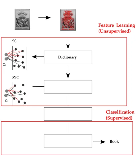
Figure 3.1 presents the object recognition system proposed in this thesis. First, features are extracted and descriptors are obtained. We use SIFT to extract features. Then, a second phase responsible to learn a sparse dictionary, is carried in an un-supervised way. After building a dictionary, we perform the coding process. In our case the coding process considers not only sparsity, but also spatial similarity, defined here as Sparse Spatial Coding (SSC). This codes are pooled using a max pooling method, forming a global feature. Finally, this image signature is presented to a learning method that could be our off-line OCL or the online LaRank.

✸✳✶ ❋❡❛t✉r❡ ❊①tr❛❝t✐♦♥

Choosing the appropriate feature is a critical step in object recognition methodolo-gies. In this work, we will follow an approach that is similar to Fei-Fei and Perona [2005], which models the extraction phase by a collection of local patches. Each patch will be used to construct a signature defining a word to build our dictionary.

3. METHODOLOGY 18

Dictionary

Sparse Spatial Coding

Global Feature

Learning Classifier (1) Feature extraction

(2) Unsupervised Feature dictionary learning

(3) Coding (SSC)

(4) Spatial Pooling

(5) Classification Method, online learning or OCL.

SC

Xi

Feature Learning (Unsupervised)

Classification (Supervised)

Book

SSC

Xi

Figure 3.1: Object recognition system overview. First image descriptors are ob-tained, followed by the dictionary learning module, then the SSC coding process is performed, encapsulated by the feature learning module. Finally, these codes are pooled and send to a classifier, an off-line OCL, proposed in this work, or an online learning approach.

3. METHODOLOGY 19

✸✳✶✳✶ ❙■❋❚ ❉❡s❝r✐♣t♦r

Lowe, in his landmark paper [Lowe, 2004], presents a keypoint detector as well as an algorithm to create a descriptor for each keypoint. In this text we will focus on the descriptor assembly procedure, since we did not use the detector. The standard SIFT descriptor is a vector of size 128 floats which is created in two main steps:

1. Orientation assignment and,

2. Descriptor assembly.

In the first step, local gradients are computed in a patch of sizet×t, by default

t=16. The orientationθ(x,y)of each pixel patch is computed as:

θ(x,y) =arctan

I(x,y+1)−I(x,y−1) I(x+1,y)−I(x−1,y)

and its magnitudem(x,y)

m(x,y) = q[I(x+1,y)−I(x−1,y)]2_{+ [I(x,y+1)−I(x,y−1)]}2_,

where I is the image in the closest scale where the patch is located.

The patch is subdivided in t regions and the local gradients are weighted by a Gaussian window. Each region has a histogram with 8 orientation bins and these histograms are formed by taking the weighted values around the patch. The domi-nant direction of each region correspond to the highest peak in histograms.

The 8 bins of allt histograms are concatenated forming the 128-vector, which after normalization, represents the SIFT descriptor. The whole procedure makes the descriptor scale and rotation invariant due to the histogram based on scale and a canonical orientation, and robust to illumination changes thanks to normalization.

Algorithm 1SIFT_descriptors = Calculate_Feature () Require: Images,grid_space,patch_size,Max_img_dim

1: fori =1→Image.totaldo

2: image =read_image(i);

3: ifimage.widthorimage.length> Max_img_dimthen

4: image = im_resize(Max_img_dim); {perform a bicubic interpolation.} 5: end if

6: grids =obtain_patches(image.widthorimage.length,patch_size,grid_space);

3. METHODOLOGY 20

Algorithm 1 is responsible for the feature extraction. The process consists of reading the whole set of images, checking for images that are beyond the specified maximum size, resizing if necessary, followed by the image division into patches. From these patches, we obtain SIFT descriptors, that feed our unsupervised dictio-nary learning module.

✸✳✷ ❯♥s✉♣❡r✈✐s❡❞ ❢❡❛t✉r❡ ❧❡❛r♥✐♥❣

In linear generative models for images, each imagexis represented by a linear com-bination of basis functions, that in our case are columns of a dictionary (D), by blending D_i columns with weight µi in the aim to infer the vector µ to better

re-construct the input xusing a dictionary D, is given by:

x =

∑

this equation can be solved, obtaining the representationµ, if the number of dictio-nary elements is equal in size to input. So applying the inverse of the dictiodictio-nary to the input, result in µ,

µ =D−1x. (3.2)

Sparse code methods present an overcomplete dictionary D (dictionary ele-ments are much greater than input dimensionality), hence there are many solutions forµand a sparsity regularization term ofµis used to reach a single solution. Mod-els like that have been proposed in the literature, represented as a compound func-tion:

T= R(x,Dµ) +s(µ), (3.3)

where R measure the reconstruction accuracy of the method and s the sparsity of

µ. Almost all methods agree to use as reconstruction measure the squaredl2 of the difference between the input signal and the model reconstruction kx−Dµk2₂. As sparsity measure, three ways were reported in the literature,l0 norms(µ) =λ|µ|₀,

l1 norm, applied in this work, s(µ) = λ|µ|₁ and a less usual form with logarithm

s(µ) =log 1+µ2.

feature-3. METHODOLOGY 21

sign search algorithm [Lee et al., 2006].

A drawback of unsupervised feature learning when compared with the su-pervised counterpart is that, in unsusu-pervised learning, an empirical risk (usually a convex loss) is minimized, so that the linear model fits some training data, and we expect the learned model to generalize well on new data points. However, due to possible small numbers of training samples and/or a large number of predictors, overfitting can occur, meaning that the learned parameters fit well the training data, but have a bad generalization performance. This issue can be solved by making a priori assumptions on the solution, naturally leading to the concept of regulariza-tion.

✸✳✷✳✶ ❉✐❝t✐♦♥❛r② ▲❡❛r♥✐♥❣

We now move to the dictionary learning phase. The problem of learning a basis set can be formulated as a matrix factorization problem. More specifically, given a training set of signals X=x1, ...,xn inRm×n, in our case a set of SIFT descriptors, one looks for a matrix D in Rm×p, where p stands for the number of bases of our dictionary, such that each signal permits a sparse decomposition inD.

argmin

U,D n

∑

i=1

xi−µiD

2

+λ|µi|, (3.4)

where U and D are convex sets and nis the number of features. Specifically U =

{µ1. . .µn}is the set of basis weight of each descriptor inU ⊆ Rn andλis a sparsity regularization term. The number of samples n is generally larger than the signal dimension m, which ism = 128 because of SIFT andn ≥ 200000 for our validation tests. Usually, we also have p ≪n, based on samplesn=200000 andp=1024, but each signal is reconstructed using few columns from D in its representation. Note that overcomplete dictionaries with p>mare permitted.

Now we will present other matrix factorization algorithms to dictionary learn-ing.

✸✳✷✳✶✳✶ ❱❡❝t♦r q✉❛♥t✐③❛t✐♦♥ ✲ ❍❛r❞ ❆ss✐❣♥♠❡♥t

Vector quantization or clustering, can also be seen as matrix factorization problem. Given ndata vectors X = x1, ...,xn , the method looks for pcentroids {d1, ...,dp}

and a binary assignment for each vector, which can be represented by a binary vector

3. METHODOLOGY 22

Once assignments have binary values, it use the terminology clustering with hard assignment.

With these assumptions in hand, we rewrite the problem:

argmin

D,Uǫ{0,1}n

n

∑

i=1

xi−µiD

2 s.t.

p

∑

j=1

µi_j =1, for all iǫ[1,p]. (3.5)

This is the same optimization problem performed by the K-means algorithm. Moreover, the K-SVD algorithm [Aharon and Bruckstein, 2006] for dictionary learn-ing is presented by the author as a generalization of K-means, reinforclearn-ing the link between clustering and dictionary learning. Specifically, this method can be seen as a matrix factorization problem, where the columns ofµare forced to have a sparsity of one.

✸✳✷✳✶✳✷ ❱❡❝t♦r q✉❛♥t✐③❛t✐♦♥ ✲ ❙♦❢t ❆ss✐❣♥♠❡♥t

Another possible view for vector quantization is to model data vectors as non-negative linear combinations of centroids that sum to one. The corresponding opti-mization problem is

argmin

D,UǫRn

n

∑

i=1

xi−µiD

2 s.t.

p

∑

j=1

µi_j =1, for all iǫ[1,p]andµ ≥0, (3.6) which is more similar to dictionary learning than vector quantization.

Yang et al. [2009b] explore this model to computer vision in BoF models, using dictionary learning instead of vector quantization for building visual dictionaries for object recognition.

✸✳✷✳✷ ❙♦❧✈✐♥❣ ❉✐❝t✐♦♥❛r② ▲❡❛r♥✐♥❣

Sparse coding provides a class of algorithms that learn basis functions from unla-beled input data, capturing their high-level features. Sparse coding can be learned from overcomplete basis set, where the number of basis are greater than the input dimensionality. Sparse coding can model inhibition between bases by sparsifying their activation, with biological similarity to the virtual cortex model [Olshausen and Field, 1997, 2004].

simul-3. METHODOLOGY 23

taneously, but convex in U when D is fixed and vice-versa. The solving approach consists of optimizing the sparsity subset with a L1-regularized least square prob-lem and the reconstruction part with a L2-constrained least square probprob-lem. We assume L1 penalty as the sparsity function, once L1 regulation is known to produce sparse coefficients and can be robust to irrelevant features [Ng, 2004].

✸✳✷✳✷✳✶ ❙♦❧✈✐♥❣ ✇✐t❤ ❉ ✜①❡❞

When the dictionaryDis fixed Eq. 3.4 can be rewritten as:

argmin µ

n

∑

i=1

xi−µiD

2 2

| {z }

L2 constraint reconstrution

+ λ|µi|

| {z }

is a regularization parameter

, (3.7)

where the L2 constraint denotes reconstruction and λ is a regularization parame-ter, that prevents overfiting. Considering only non-zero coefficients, this reduces Eq. 3.4 to a standard unconstrained quadratic optimization problem (QP) which can be solved analytically. The algorithm tries to search for signs of coefficientsµi, given any such guess and systematically refines the guess if it turns out to initially incorrect.

✸✳✷✳✷✳✷ ❙♦❧✈✐♥❣ ✇✐t❤ ❯ ✜①❡❞

We will present how to solve the optimization problem whenU is fixed. The prob-lem is reduced to a least squares with quadratic constraint:

argmin

D n

∑

i=1

xi−µiDk

2

F (3.8)

s.t. kD_kk ≤ 1, 1≤k ≤n.

It is solved using a Lagrange Dual, since solving the dual uses significantly fewer optimization variables than the primal [Lee et al., 2006].

3. METHODOLOGY 24

✸✳✸ ❈♦❞✐♥❣ Pr♦❝❡ss

Sparse coding has been presented as a good alternative to VQ, once it is more ef-fective in feature quantization. Nevertheless, some limitations are observed in pure sparse coding methods. First, sparse coding methods are sensitive to the variance of features. Another limitation is that the L1 regularization can select quite different bases for similar patches to favor sparsity, in this way losing relationships between codes. Thus, spatial similarity can reinforce that analogous input signals will have similar column activations, resulting in similar codes.

To improve the relationship between local features and to impart more robust-ness to coding process, we introduce the SSC. In addition, SSC considers spatial similarity among features instead of just sparsity. We introduce this constraint to preserve consistency in sparse coding, for similar local features. Thus, SSC codes for local features are no longer independent.

Instead of coding with a sparsity constraint, we have chosen to use the spatial Euclidean similarity, based on the works of Wang et al. [2010] and Yu and Zhang [2009], which suggest that locality produces better signal reconstruction.

In VQ each descriptor is represented by a single base. However, spatial ap-proaches use multiple basis in order to capture possible correlations between similar descriptors.

Other feature presented by the works of Wang et al. [2010] and Yu and Zhang [2009], which led us to opt for this type of coding, is that locality gives a higher probability of selecting similar basis for similar patches. This is different from a SC approach, in which regularization can select quite diverse basis for similar patches (see Figure 3.2).

Coding with spatial sparse coding, instead of sparse coding, transforms Eq. 3.4 into:

argmin µ

n

∑

i=1

xi−Dµi

2

+λdi⊙µi2 (3.9) s.t. µi =1, ∀i,i =1, ..,n,

where ⊙ is the element by element multiplication and di is the spatial similarity member computed as

di =dist(xi,D), (3.10) and dist(xi,D) is a vector of Euclidean distances between each input descriptor xi

3. METHODOLOGY 25

SC

D={dj} j=1, ..., n

X

X

D={dj} j=1, ..., n

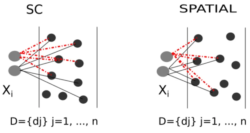
Figure 3.2: The SC shortcoming is that regularization can select different basis for similar patches, a problem that spatial constraint techniques are able to overcome.

X_irepresent the input features andDrepresents the dictionary. As it can be seen in this example, the spatial sparse coding selects the nearest basis in the dictionary.

Given these distances, we apply a KNN method that returns the Nmost simi-lar basis for the given input, leading to a low computational demand to our coding process. The values of di are normalized by themax distance to adjust the range of possible represented numbers within the interval (0, 1].

After coding each local feature, we perform a max pooling method to concate-nate each code into a final image representation.

✸✳✹ P♦♦❧✐♥❣

Pooling is used to provide invariance to image transformation and robustness to noise and clutter in a way that preserves relevant information while removing spu-rious data.

To provide a better discriminative signature, we use high dimensional local features, which are SIFT descriptors obtained from a patch of 16×16 processed over a grid space of 6 pixels between each area. We decide to make use of dense regular grid, in opposition to interest points, based on the comparative evaluation made by [Fei-Fei and Perona, 2005], who present advantages of dense features for scene recognition tasks.

First of all, the final signature has a dimensionality defined by the function:

Sizesignature=dictionarysize× T

∑

i=1

3. METHODOLOGY 26

whereTis the number of scales, in our case 3, and the pyramid scales are[1, 2, 4], so that we have a dictionary size of 1024 basis. Our final signature is 1024×(12+22+

42) =21504 vector elements per image.

Then the pooling process is applied to each scale and performs a maximization of SSC codes. Let U be the result of the application of Spatial Sparse Coding (Eq. 3.9) to a set of descriptor X, with a trained dictionary D. We build the final image signature with a functionP

z =P(U), (3.12)

wherePis a pooling function defined on each column ofU. Recall that each column ofUcorresponds to the response to the entire set of descriptor to a specific column ofD. In our work, we choose as pooling function to maximize the SSC codes

z_j =maxu_1j,u_2j,u_3j, ...,u_Mj , (3.13) wherez_jis the j-th element of z,u_i,jis the element from the columnjand lineifrom U, and Mis the number of local descriptors per area. We have chosen this function, despite average pooling once the works of Liu et al. [2011]; Boureau et al. [2010b] prove that max pooling presents state-of-the-art results. In addition, we perform max pooling in a spatial pyramid image representation. It is preferable, since max pooling under different locations and spatial scales provide more robustness to local transformations. Algorithm 2 summarizes the process.

The final representation is sent to some of our classification methods. First, we try the final signature with a proposed off-line method. We then use an online

Algorithm 2SSC = Pooling (X,D,Pyramid,Knn)

1: Ind=0;

2: SSC_codes =SSC(D,X,Knn); {Coding with spatial similarity}

3: forLevel =1 →Pyramid.levelsdo

4: Find_local_Feature(X,Level); {Find to which region of interest each local fea-ture belongs}

5: forROI =1→Number of ROIsdo

6: ind=ind+1;

7: B(:,ind) = max(SSC_codes(id_ROI));

8: end for

9: end for

3. METHODOLOGY 27

approach that comprises the final version of the methodology.

✸✳✺ ❖✛✲❧✐♥❡ ❧❡❛r♥✐♥❣ ♠❡t❤♦❞

We propose an off-line classification method based on Singular Value Decomposi-tion (SVD), called Orthogonal Class Learning (OCL), that takes advantage of the high dimensionality of the feature vectors when compared to the number of feature examples, i.e., we have a set with t n-dimensional feature vectors wheren ≫ t. In this case, a base with onlytcomponents is used to represent new feature vectors. In addition, we obtain a new base for which new feature vectors are unit vectors, and pairwise orthogonal.

Consider, initially, we have h classes, each of which represented by k n -dimensional feature vectors so that we have t = h ×k feature vectors. Let

f₁, f2, . . . , ft denote feature vectors of all training data and let F denote the n×t

matrix where columns are formed by the feature vectors, that is,

F = (f1, f2, ..., ft). (3.14)

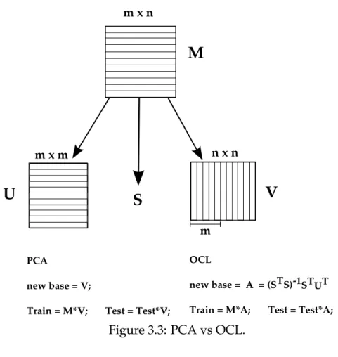
Using SVD decomposition, we have that F = USVT. Instead of forming new basis from columns ofU as usual PCA, we use the fact that

VT = (STS)−1STUTF, (3.15) and form a new base A = (STS)−1STUT such that, in this new base, our new fea-ture vectors are columns fromVT, being unit vectors and pairwise orthogonal. The advantage of this new representation is that, given object classes i and j and their feature vectors as matrices F_i and F_j formed with columns from F, we obtain new matrices C_i = A.F_i and C_j = A.F_j, such that columns of C_i and C_j are pairwise orthogonal vectors. Figure 3.3 depicts the difference between PCA and OCL.

Finally, we construct our classifier based on the aforementioned observations. Given an object and its feature vector f, we obtain new feature vectore = A×f and the decision over the class Sis given by

S=argmax

s

kC_sTek. (3.16)

3. METHODOLOGY 28

M

m x n

U

_S

V

n x n m x m

m

PCA

new base = V;

Train = M*V; Test = Test*V; OCL

new base =

Train = M*A; Test = Test*A; A = (STS)-1STUT

Figure 3.3: PCA vs OCL.

Algorithm 3OCL classification(label) Require: nt,tr,ts

1: Training procedure

2: [USV] =svd(tr);

3: tr =V; {V turns the new train set on new space}

4: A= (STS)−1STUT {A turns new basis}

5: Test procedure

6: ts =ts∗A{pass the test set to new basis}

7: forj =1→all test examplesdo

8: fori =1→each class clusterdo

9: t1=ts(j);

10: l =t1∗tr((i−1)∗nt +1 :i∗nt, :);

11: n(i) =norm(l, 2);

12: end for

13: [v,p] = max(n); {find the highest norm l2 of the classes}

14: label(j) = p; {Prediction}

3. METHODOLOGY 29

✸✳✻ ❖♥❧✐♥❡ ❧❡❛r♥✐♥❣ ♠❡t❤♦❞

The approach used in our final methodology was based on the Online LaRank [Bor-des et al., 2008]. We have selected a LaRank multi-class solver. The LaRank rithm is grounded in a randomized exploration, inspired by the perceptron algo-rithm [Bordes et al., 2007].

LaRank was selected as a solver, among other options, for the following rea-sons:

• Reaches equivalent accuracy values with less computational consumption when compared to other SVM solvers, like SVMstruct [Tsochantaridis et al., 2005];

• Generalizes better than perceptron-based algorithms;

• Achieves nearly optimal test error rates after a single pass over the randomly reordered training set.

The Online LaRank technique achieves the same test accuracy of batch opti-mization after a single epoch thanks to a reprocess step implementation over SMO-Optimization algorithm of Platt [1999].

In order to clarify how a SVM works we will give a overview of this method.

✸✳✻✳✶ ❙❱▼

Support Vector Machines are based on the concept of hyperplane as boundaries. A hyperplane is used to split different class sets. Usually, a good separation is achieved by an hyperplane which has the greatest distance among the nearest data point of each class, called Maximum margin. According to Alpaydin [2010], from all possible linear decision function, the one that maximizes the margin of the training set will minimize the generalization error in a noise free dataset. Figure 3.4 exemplifies this case. Moreover, the training points that are nearest to the split function (shown by red circles) are named Support Vectors (SV).

Nevertheless, often data is not linearly distinguishable and, then, non-linear manifolds are needed to divide the data. For instance a XOR operation requires a radial function to be separable.

We choose SVM for our final learning method based on some properties:

3. METHODOLOGY 30

SV

SV SV

SV

SV

Figure 3.4: The Figure above presents an example of two classes where a hyperplane separates them in two classes (circles and squares).

• Linear SVM presentsO(n)in training (scale linearly with the size of the train-ing set):

– Efficiency to deal with extra large sets;

– Works with high dimensional data;

❈❤❛♣t❡r ✹

▼❡t❤♦❞ ❱❛❧✐❞❛t✐♦♥

For evaluation purposes, we tested our method in two scenarios. First, we per-formed experiments using our technique with off-line classification methods, such as SVM, and with the OCL approach developed for this work. We then tested our final methodology (Sparse Spatial Coding) with an online learning algorithm, an SVM solver called OLarank [Bordes et al., 2008].

First, a parameter analysis is performed to show the effects of changing their values, also presenting when each parameter maximizes system performance. We first test our method with our off-line classification method, showing that only a sparse spatial constraint approach can lead to state-of-the-art results. We then show that the combination of sparse coding and locality with the correct online learning method can produce superior results.

✹✳✶ P❛r❛♠❡t❡r ❙❡tt✐♥❣s

One of the most critical setting for an object recognition method is the choice of a local feature to be used. In our experiments we chose SIFT [Lowe, 2004] due to its high accuracy on several object recognition tasks [Boiman, 2008; Yang et al., 2009b; Lazebnik et al., 2006]. Because of the dense grid sampling in the step for selecting regions of interest, our experiments use 6 pixels step between each region and a patch size of 16×16 pixels. During our experiments we tested the system with smaller step sizes, such as 4 and 2, as discussed in section 4.1.1.3. Our best results were with 4 pixels step; however, to make a fair comparison with the literature, which uses 6 pixels space. We report results with 6 pixels between patches and subsequently with 4. We also resize the images to 300×300 pixels.

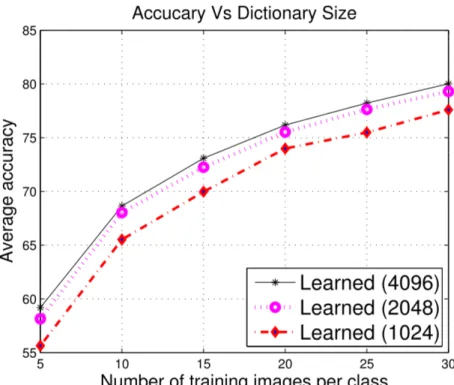
We trained, by default, all the dictionaries for the tests with 1024 basis and