Bayesian inference of mixed models in quantitative genetics of crop species

VINÍCIUS RIBEIRO FARIA

Bayesian inference of mixed models in quantitative genetics of crop

species

Tese apresentada à Universidade Federal de Viçosa, como parte das exigências do Programa de Pós-Graduação em Genética e Melhoramento, para obtenção do título de Doctor Scientiae.

VIÇOSA

Ficha catalográfica preparada pela Seção de Catalogação e Classificação da Biblioteca Central da UFV

T

Faria, Vinícius Ribeiro, 1983-

F224b Bayesian inference of mixed models in quantitative 2012 genetics of crop species / Vinícius Ribeiro Faria.

– Viçosa, MG, 2012.

viii, 27f. : il. ; 29cm.

Inclui apêndice.

Orientador: José Marcelo Soriano Viana.

Tese (doutorado) - Universidade Federal de Viçosa. Referências bibliográficas: f. 18-22.

1. Genética quantitativa. 2. Plantas - Melhoramento genético. 3. Modelos lineares (Estatística). 4. Monte Carlo, Método de. 5. Teoria bayseiana de decisão estatística.

I. Universidade Federal de Viçosa. Departamento de

Fitotecnia. Programa de Pós-Graduação em Genética e

Melhoramento. II. Título.

VINÍCIUS RIBEIRO FARIA

Bayesian inference of mixed models in quantitative genetics of crop

species

Tese apresentada à Universidade Federal de Viçosa, como parte das exigências do Programa de Pós-Graduação em Genética e Melhoramento, para obtenção do título de Doctor Scientiae.

APROVADA: 30 de julho de 2012.

Prof. Fabyano Fonseca e Silva (Coorientador)

Dr. Marcos Deon Vilela de Resende (Coorientador)

Dr. Lauro José Moreira Guimarães Prof. Pedro Ivo Vieira Good God

AGRADECIMENTOS

À Universidade Federal de Viçosa, pela oportunidade de realizar este curso. À Capes e ao CNPq, pelo auxílio financeiro.

Aos meus orientadores Marcelo e Fabyano, pelo apoio, pela confiança e pela amizade.

Aos demais componentes da banca, pelas valiosas sugestões.

Aos colegas de trabalho de campo, pela colaboração e pela agradável convivência.

A todos os amigos, com os quais convivi desde os tempos de graduação, e aos tantos companheiros de república.

BIOGRAFIA

VINÍCIUS RIBEIRO FARIA, filho de Jandir de Faria e Célia Ribeiro de Faria, nasceu na cidade de Dores do Indaiá - MG, em 22 de outubro de 1983.

Realizou os estudos do primeiro e segundo graus, na Escola Estadual Benjamim Guimarães e na Escola Estadual Francisco Campos, respectivamente, até o ano de 2001.

Ingressou no curso de Agronomia no ano de 2002 na Universidade Federal de Viçosa.

Em outubro de 2006 obteve o diploma de Engenheiro Agrônomo pela Universidade Federal de Viçosa.

Em 2006 iniciou o Programa de Mestrado em Genética e Melhoramento, pela mesma instituição, com ênfase em Genética Quantitativa e Melhoramento de Milho-Pipoca, submetendo-se à defesa de dissertação em julho de 2008.

SUMÁRIO

RESUMO vii

ABSTRACT viii

1. Introduction 1

2. Materials and methods 4

2.1. Experimental data

4

2.2. Model and Bayesian inference

4

2.3. Computational features

7

2.4. Informative prior distributions

9

2.5. Bayesian analysis

12

3. Results 13

4. Discussion 15

5. References 18

RESUMO

FARIA, Vinícius Ribeiro, D.Sc., Universidade Federal de Viçosa, julho de 2012. Inferência bayesiana de modelos mistos em genética quantitativa de espécies vegetais. Orientador: José Marcelo Soriano Viana. Coorientadores: Fabyano Fonseca e Silva e Marcos Deon Vilela de Resende.

Predição de valores genéticos e componentes de variância via Inferência Bayesiana ainda são raras no melhoramento de culturas anuais. Desse modo, os objetivos deste trabalho foram implementar uma estrutura Bayesiana para análise de modelos mistos aplicada ao melhoramento de espécies anuais e explorar diferentes possibilidades no uso de informações à priori. Para ilustrar as ferramentas da Inferência Bayesiana no melhoramento de culturas anuais foram utilizados os dois primeiros ciclos de seleção de famílias de meios-irmãos da população de milho pipoca Viçosa. As ferramentas estatísticas utilizadas foram o software JAGS e o pacote R2jags. Priores não informativas e informativas com base na meta-análise para o inverso dos componentes de variância foram utilizadas na análise dos dados do primeiro ciclo. Para o segundo ciclo, priores não informativas e informativas obtidas a partir das distribuições à posteriori das duas análises do primeiro ciclo foram utilizadas, totalizando três diferentes análises. Em relação ao primeiro ciclo, a utilização de priores informativas por meio de meta-análise forneceu resultados claramente distintos em relação ao uso de priores não informativas apenas para a produção de grãos. Em relação ao segundo ciclo, os resultados para capacidade de expansão e produção de grãos mostraram diferenças entre as três análises. As diferenças entre as análises foram restritas aos componentes de variância e herdabilidade. As correlações entre os valores genéticos preditos foram quase perfeitas (0,99) e a coincidência entre os 20 pais superiores de pelo menos 90%.

ABSTRACT

FARIA, Vinícius Ribeiro, D.Sc., Universidade Federal de Viçosa, July, 2012. Bayesian inference of mixed models in quantitative genetics of crop species. Adviser: José Marcelo Soriano Viana. Co-Advisers: Fabyano Fonseca e Silva and Marcos Deon Vilela de Resende.

Bayesian prediction of breeding values and genetic variances are still scarcer in annual crop breeding. The objectives were to implement a Bayesian framework for mixed models analysis applied to crop species breeding and to exploit different possibilities of informative prior elicitation. The Bayesian inference in annual crop breeding was illustrated with the first two half-sib selection cycles in the popcorn population Viçosa. The Bayesian framework was based on the JAGS software and the package R2jags. For the first cycle, non-informative prior for the inverse of the variance components and informative prior based on meta-analysis were used. For the second cycle, non-informative prior and informative prior defined as the posterior from the non- and informative analyses of the first cycle were used. Regarding the first cycle, the use of a informative prior from meta-analysis provided clearly distinct results relative to the analysis with non-informative prior only for grain yield. Regarding the second cycle, the results for expansion volume and grain yield showed differences between the three analyses. The differences between the non- and informative prior analyses were restricted to variance components and heritability. The correlations between the predicted breeding values were almost perfect (0.99), determining coincidence between the 20 superior parents of at least 90%.

1. Introduction

The best linear unbiased prediction (BLUP) (Henderson 1974) has been widely used for genetic evaluation in animal and forestry breeding programs. A common approach for variance components estimation is the restricted maximum likelihood (REML) (Patterson and Thompson 1971). Bayesian prediction of breeding values and genetic variances has been also largely employed (Sorensen 2009; Blasco 2001). Actually, REML/BLUP and/or Bayesian inference have additional relevant applications in genetics and breeding, as prediction of breeding values using genome-wide dense marker maps (Meuwissen et al. 2001), mapping QTLs (quantitative trait loci) (Bink et al. 2008), analysis of population structure (Pritchard et al. 2000), association mapping (Marttinen and Corander 2010) and inferring levels of gene expression and regulation (Beaumont and Rannala 2004).

However, only recently the annual crop breeders have recognized the advantages of the genetic evaluation by BLUP or Bayesian analysis, as variance components estimation based on method superior for unbalanced data, relevance of historical data and pedigree information to increase the prediction accuracy, and possibility of inclusion of prior information on the parameters to be estimated (Ye et al. 2007; Piepho et al. 2008; Atkin et al. 2009; Bauer et al. 2009; Viana et al. 2012a). Bauer et al. (2006), Flachenecker et al. (2006), Oakey et al. (2007) and Viana et al. (2010a, b; 2011a, b), among others, have demonstrated that BLUP has applications in recurrent intra- and interpopulation breeding programs, and in the development of pure/inbred lines.

accounting for relatedness between lines and the genotype-by-environment interaction was superior. As most Bayesian analyses in genetics and breeding, there was not inclusion of the prior knowledge. Fortunately, all Bayesian analysis for genetic evaluation in animal and forestry breeding are adequate to annual crop breeding. Waldmann and Ericsson (2006) and Waldman et al. (2008) fitted a multi-trait individual model and the additive-dominant model for partial diallel analyses of real and simulated data of Scots pine progeny. Differences between REML and Gibbs sampling estimates occurred for both data. With high dominance, the additive-dominant model had the best fit. With low dominance, an informative prior was necessary to avoid overestimation of the dominance variance.

The Bayesian approach has some advantages as flexibility in choosing distributions for sample data and unknown parameters, facilities in interval estimation and possibility of incorporate prior knowledge about the parameters of interest (Sorensen 2009; Blasco 2001). Although this latter advantage is widely mentioned in literature as a potentially attractive feature of Bayesian inference (Beaumont and Rannala 2004), it has been underexplored in a practical viewpoint in animal and plant breeding, perhaps because of lack of situations in which this previous knowledge can be naturally incorporated. In our viewpoint too, the incorporation of background information represents a special feature of Bayesian analysis in crop species breeding, since the concept of selection cycles characterizes a natural mechanism for informative prior elicitation. It is because the posterior distribution for the parameters of interest, like variance components, from a given cycle, could be used as prior distribution in the analysis of the next cycle, thus forming a knowledge update system.

for crop breeding data analysis because they do not support especial relationship structures as those from family-based designs and additional random effects like dominance. Furthermore, these software have no flexibility in choosing distributions for data and parameters, avoiding, respectively, the use of non-normal distributions and informative prior distributions based on previous analysis. One attractive solution is the software WinBUGS, which are a general Bayesian programming environment, highly flexible in relation to these mentioned models and distributions (Lunn et al. 2009). Damgaard et al. (2007) and Waldmann (2009), respectively in animal and plant breeding, have implemented mixed models analysis in this software, but it does not allows a direct handling of incidence and relationship matrices from mixed model equations, being necessary using indirect ways based on algebraic notations that decreases the computational efficiency. One interesting alternative is the JAGS (Just Another Gibbs Sampler) software (Plummer 2012), which has the same flexibility and facilities of WinBUGS, but with the advantage of allowing a matrix language programming.

2. Materials and methods

2.1. Experimental data

The Bayesian inference in annual crop breeding was illustrated with the first two half-sib selection cycles in the popcorn population Viçosa. The two trials with 196 progenies were designed as a 14 x 14 simple lattice and performed in the experimental station of the Federal University of Viçosa (UFV) at Coimbra, Minas Gerais state, in the 1999/2000 and 2001/2002 growing seasons. Each plot corresponded to a 5 m row with 25 plants (ideal stand). The traits analyzed were expansion volume (EV) and grain yield.

2.2. Model and Bayesian inference

In agreement with the experimental design, in the present study was fitted the following mixed model

1 1 2 2

= + + + ,

y Xβ Z u Z u e

(Eq. 1) where y is the vector of phenotypic values, X and  are, respectively, the incidence matrix and the correspondent vector of fixed effects (population mean and replication effects),

1

Z

and Z2 _{are the incidence matrices of the random effects,} u1 _{is the vector of half of the} additive genetic value of the common parent, u2 _{is the vector of block within replication} effects and e is the residuals vector.

Assuming

2 2

e e

| ~ N(0, )

e I _{, the sample distribution of the observed data (likelihood}

function) is

1 2

2 2 2 2

1 2 u u e 1 1 2 2 e

| , , , , , ~ N( + + , )

y β u u Xβ Z u Z u I

(Eq. 1.1)

where

2 A 2

u₁ (1/4)



and

2 A

The prior distributions for the location parameters (fixed and random effects) of the model were given by

2 2

β β β β β β

| , ~N( , )

β μ I μ I

(Eq. 1.2)

1 1

2 2

1| u ~N( , u )

u A 0 A

(Eq. 1.3)

2 2

2 2

2| b u ~N( , b u )

u I 0 I

(Eq. 1.4)

where μβ and 2

β _{are the known parameters (hyperparameters) of a multivariate}

normal distribution with covariance matrix given by 2 β β

I

, in which Iβ is a diagonal matrix; A = {2rij} is the additive relationship matrix and rij is the coefficient of coancestry between the common parents of progeny i and j; Ib is a diagonal matrix, which represents the

independence between blocks within replications. For the variance components 1 2 u _{, 2}

2 u _and 2

e_{, the following scaled inverted chi-square distributions were assumed, respectively, as} prior,

u1

2 -2

u1|ν ,S ~ ν S χu1 u1 u1 u1 ν _{(Eq. 1.5)}

u2

2 -2

u2|ν ,S ~ ν S χu2 u2 u2 u2 ν _{(Eq. 1.6)}

e

2 -2

e|ν ,S ~ ν S χe e e e ν _{. (Eq. 1.7)} Under the Bayes’ Theorem, the joint posterior distribution of all unknown parameters

( 1 2

2 2 2

1 2 u u e

, , , , and

β u u

) is proportional to the product of the likelihood function (Eq. 1.1) and the prior distributions (Eq. 1.2 to 1.7). Thus, the general formulation of this theorem is



 





















 



1 2 1 2 1

2

2 2 2 2 2 2 2 2

1 2 u u e 1 2 u u e β β 1 u

2 2 2 2

u1 u1 u1 2 b u u2 u2 u2 e e e P , , , , , | P | , , , , , P | , P |

P |ν ,S P | P |ν ,S P |ν ,S .

   

  

β u u y y β u u β μ u A

u I





 









 

   

 

 

1 2 u u1 β 1 1 1 1 t -N

1 1 2 2 1 1 2 2

2 2 2 2 2

1 2 u u e e 2

e

t

-n ν

-n t ₁

β β 2

2 2 2 1 1 2 2 u1 u1

β 2 u 2 u

β u u

y- + + y- + +

P , , , , , | exp

2

- - _{ν S}

exp exp exp

2 2 2

      _{ }       _{ }      _{   }       _ _       _{ } _ _{   }     _{ }  

Xβ Z u Z u Xβ Z u Z u

β u u y

β μ β μ _{u Au}

 

 

 

1

u2 u2

2 2

2 2

2

-n t ν N

1 +1

2

2 2 2 2 2 u2 u2 2 2 e e

u 2 u 2 e 2

u u e

ν S ν S

exp exp exp . Eq.(2)

2 2 2

  _ _ _    _ _ _ _                                 _{ }     u u

The statistical inference on parameters from Eq. 2 is realized on the posterior marginal distributions,P(.| )y , for each one of these parameters. Therefore, in order to obtain these distributions, the following integrals must be solved









2 2 2

1 2 -h 1 2 _{u u e}

1 2 2 2 2

h 1 2 u u e

P β |y 



P , , , , , | d d d d d d ,β u u y _{β u u}

(Eq. 2.1)









2 2 2

1 2 1 2 u1 u2 e

2 2 2

1i 1 2 u u e β _-i

P u |y 



P β u u, , , , , | d d d d d d ,y _{u u}

(Eq. 2.2)









2 2 2

1 2 1 _{u u e}

1 2 2 2 2

2 j 1 2 u u e β _2-j

P u |y 



P β u u, , , , , | d d d d d d ,y u u

(Eq. 2.3)









2 2

1 1 2 1 2 u2 e

2 2 2 2

u 1 2 u u e β

P |y 



P , , , , , | d d d d d ,β u u y _{u u}

(Eq. 2.4)









2 2

2 1 2 1 2 u1 e

2 2 2 2

u 1 2 u u e β

P |y 



P , , , , , | d d d d d ,β u u y _{u u}

(Eq. 2.5)

 





2 2

1 2 1 2 _{u1 u2}

2 2 2 2

e 1 2 u u e β

P |y 



P , , , , , | d d d d d .β u u y _{u u}

(Eq. 2.6) Since these integrals do not have analytical solutions, the MCMC algorithms can be used to generate random samples from these marginal distributions indirectly from the full conditional posterior distributions (f.c.p.d), which is the posterior distribution for a given parameter (Eq. 2) conditional on the data and the remaining parameters. In general terms,

families of probability distributions, therefore presenting closed forms, the Gibbs sampler algorithm can be used.

2.3. Computational features

The Gibbs sampler begins with θ(0), some start values for parameters, while θ(t) are the values generated at t-th iteration of this algorithm, which are obtained by collecting the

draws from each f.c.p.d

(t) (t) (t) (t-1) (t-1) k k 1 k-1 k+1 p

θ ~P(θ |θ ,...,θ ,θ ,...,θ , )y

, so that

(t) (t) (t) (t)

1 2 p

=_θ ,θ ,...,θ ._

θ

Thus, defining T as the total number of iterations, if T  the Markov chain property ensures that, after discarded some initial iterations (burn-in period), the values generated for a given parameter θk are characterized as samples from its marginal posterior distribution,

k

P(θ | ).y

After the descriptions of statistical and computational features, note that the obtaining of f.c.p.d. is a key point in Bayesian inference. Assuming normal distributions for the data and location parameters, and scaled inverted chi-square distributions for variance components, some references (García-Cortés and Sorensen 1996; Sorensen and Gianola 2002) bring a detailed mathematical handling of Eq. 2 in order to derive general classes of f.c.p.d. for some mixed models with one and two random effects. These distributions have been used in some animal breeding software like MTGSAM and gibbsf90.

Damgaard et al. (2007) and Waldmann (2009) proposed using the software WinBUGS as a flexible and easy alternative to Bayesian inference of mixed models, since its requires only specifications of the data listing, likelihood function and prior distributions. However, despite the facilities, these approaches not allowed a direct handling of incidence and relationship matrices, being necessary using alternative parameterizations based on algebraic notations that are not usual and with low computational efficiency.

1 2

2 2 2 2

1 2 u u e e

model

Y ~ dmnorm(mu[1:N,1],I[1:N,1:N]*tau_e)

| , , , , , ~ N( , ) Eq. (1.1)

mu[1:N,1] <- X[1:N,1:nbeta]%*%beta

#likelihood function

y β u u I

{



1 1 2 2

[1:nbeta,1] + Z1[1:N,1:nu1]%*%u1[1:nu1,1] + Z2[1:N,1:nu2]%*%u2[1:nu2,1]

beta[1:nb

Xβ + Z u + Z u

#prior distribution for fixed effects

 

2 2

β β β β β β

eta,1] ~ dmnorm (mean_beta[1:nbeta,1], Ibeta[1:nbeta,1:nbeta]*0.00001)

| , ~N( , ) Eq. (1.2)

β μ I μ I

#prior di

1 1

2 2

1 u u

u1[1:nu1,1] ~ dmnorm (mean_u1[1:nu1,1], A[1:nu1,1:nu1]*tau_u1)

| ~N( , ) Eq.

stributions for random effects

u A 0 A

2 2

2 2

2 b u b u

(1.3)

u2[1:nu2,1] ~ dmnorm (mean_u2[1:nu2,1], Ib[1:nu2,1:nu2]*tau_u2)

| ~N( , ) Eq. (1.4)

u I 0 I

#prior distribu

u1

2 -2

u1 u1 u1 u1 u1 ν

2 u2

tau_u1 ~ dgamma(vu1/2, Su1/2)

|ν ,S ~ ν S χ Eq. (1.5)

tau_u2 ~ dgamma(vu2/2, Su2/2)

|

tions for the inverse of variance components

u2

e

-2 u2 u2 u2 u2 ν

2 -2

e e e e e ν

ν ,S ~ ν S χ Eq. (1.6)

tau_e ~ dgamma(ve/2, Se/2)

|ν ,S ~ ν S χ Eq. (1.7)

sigma2_e <- 1/tau_e

#Definition of variance components and heritability

sigma2_u1 <- 1/tau_u1 sigma2_u2 <- 1/tau_u2 sigma2_a <- 4*sigma2_u1

h2<-sigma2_u1 / (sigma2_u1 +sigma2_e/2 )

}

Figure 1 Schematic illustration of the model file to be used in JAGS software, where Y is the phenotypic values

vector; X, Z1 and Z2 are, respectively, incidence matrices for β, u1 and u2; N, nbeta, nu1 and nu2 are,

respectively, the numbers of observations, of fixed effects, of families and of blocks; mean_beta, mean_u1 and mean_u2 are, respectively, the mean vectors of prior distributions for β, u1 and u2; I, Ibeta, A, Ib are,

respectively, matrices related with covariance of prior distributions for e, β, u1 and u2; and ν. and S. are the

In relation to prior distributions for the variance components ( 1 2 2 u , u 2 _and

2 e_{) in} Figure 1, note that is being used a reparameterization of original scaled inverted chi-square (Scale

-2

χ _{) distribution because the JAGS does not works directly with this distribution. This}

distribution is a special case of the inverse gamma distribution (inv Gamma). Thus, assuming that

2 ~ Scale χ (ν,S)-2

, where S = ν 2* and 2* is the prior most likely value to 2, one

equivalent distribution is

2 _{~ inv Gamma(ν/2,S/2)}

(Sorensen and Gianola 2002, p.85), which allows using

2

=1/ ~ Gamma(ν/2,S/2)_{as defined in Figure 1.}

2.4. Informative prior distributions

The present study also evaluated the influence of using informative and non-informative prior distributions on genetic parameter estimation. The use of prior knowledge has especial interest for Bayesian analysis in crop breeding, because the posterior distribution for the parameters (variance components) in a given selection cycle could be used as prior distribution in the analysis of the next cycle, characterizing a knowledge update system.

In order to perform the analysis involving different prior distributions, for the first cycle were initially used non-informative prior for the inverse of the variance components, defined by

2

=1/ ~ Gamma(0.001,0.001)_{. Since the same population and phenotypes were}

analyzed by ANOVA/BLUE (best linear unbiased estimation) or REML/BLUP (Arnhold et al. 2010; Viana et al. 2012a), informative prior based on meta-analysis (Whitehead 2002) was used too. This statistical method integrates the results of several independent studies, synthesizing them into a single measure. For this, the inverse of the average value of a given variance component (

2

=1/ _{) and its respective variance (} 2

S

distribution:

α =

β _and

2 2

α

S

β 

. Thus, it was possible to define 2

α=

S

and 2

2

β=

S

, resulting in

2

=1/ ~ Gamma(α,β)_{, which is an informative prior such as its expectation and variance}

are coincident, respectively, with mean and variance of the data set containing the reported values in the referenced papers.

This same system of equality was used in order to exploit the results of the first cycle as prior information for the second cycle. For this, the mean and variance of the marginal posterior distributions for the inverse of the variance components ( ) obtained from the analysis with or without informative prior were equalized to expectation and variance of a gamma distribution, from which the values of α and β were calculated. Thus, the expectation and variance of these gamma distributions are coincident, respectively, with mean and variance of the posterior distributions from the first cycle, characterizing an incorporation of prior knowledge coming from the previous cycle.

A total of three analyses were performed for each trait in the second cycle: non-informative prior using

2

=1/ ~ Gamma(0.001,0.001)_{; informative prior defined as the}

2.5. Bayesian analysis

3. Results

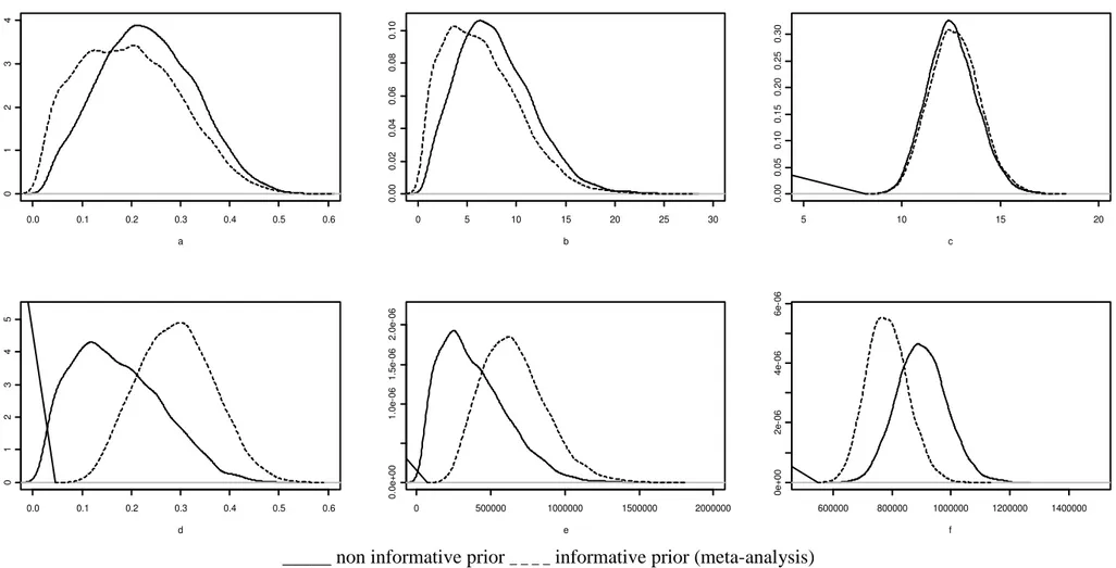
In relation to convergence criteria, it was verified that the absolute values of Geweke's Z statistics were below 1.96, and the dependence factor of Raftery and Lewis were below 5.0 for all parameters, indicating its convergence (Tables 1 and 2). Regarding the first cycle, the analyses of EV showed that the use of a informative prior from a meta-analysis did not provided clearly distinct results relative to the analysis with non-informative prior (Table 1). The estimates and precision of the genetic parameters were equivalent, since the values of standard deviation and 95% HPD (high probability density) interval were similar. However, for grain yield both analyses provided distinct results. For additive variance and heritability the analysis with prior information provided estimates 1.7 times higher than those found when we used non-informative prior and there was an increase in precision. The coefficient of variation for the additive variance and heritability decreased from 58.9 to 33.1% and from 52.3 to 26.4%, respectively.

The differences between the two analyses are highlighted from the posterior densities of the genetic and non-genetic parameters (Figure 1). For EV there was a tendency of overlapping between the curves, indicating little influence of the prior information. However, for grain yield the difference in the distributions promoted by the inclusion of prior information was evident. In the analysis with prior information the distributions were more symmetric compared to the analysis without prior information.

decreases in the standard deviations were 40.7 and 45.7 for the additive variance, and 48.2 and 49.0 for heritability. The posterior densities of the genetic and non-genetics parameters with prior information have a higher probability density for the mean value compared to the analysis without prior information (Figure 2).

In relation to grain yield, there were differences in the estimates and precision of the variance components and heritability (Table 2). The inclusion of prior information clearly determined lower heritability and more precise estimates of the additive variance and heritability. However, compared to the analysis with non-informative prior, there was relevant decrease (42.0%) in the estimate of the additive variance with informative prior and posterior from cycle 1, and significant increase (59.6%) with informative prior and posterior from cycle 1 with meta-analysis. By visual analysis of the posterior densities it is also evident that there are differences between the three analyses, since the highest probability densities are at different values for all parameters (Figure 2).

4. Discussion

We will ignore here, intentionally, any comparison between Least Squares/BLUE (best linear unbiased estimation), REML/BLUP and Bayesian inference for estimation or prediction of genetic parameters. Since breeders in general are interested in tools to increase selection efficiency, it is not necessary again to discuss on the most efficient statistical approach for genetic evaluation. First because we have only one balanced dataset and second because none approach should be systematically superior in all situations. As stated by Blasco (2001), both Bayesian and frequentist schools of inference are well established, neither of them has, in general, operational difficulties, and there is software available to analyze a large variety of problems from both points of view. However, we should show that with an adequate statistical tool, it is possible, although not necessarily ease, to use Bayesian inference for genetic evaluation in crop species, as we and others have done with REML/BLUP (Bauer et al. 2006; Flachenecker et al. 2006; Oakey et al. 2007; Viana et al. 2010a, b; 2011a, b), using the ASReml (Gilmour et al. 2009) and SAS (Littell et al. 2006) software.

Giannotti (2002) also recommended meta-analysis techniques for quantitative reviews of genetic parameters.

In recurrent intra- and interpopulation breeding programs and in the development of pure/inbred lines the priori information for a given selection cycle should be based on the posterior distribution of the parameters from the previous cycle. Wang et al. (1993) showed that the parameter estimates were more precise when using higher levels of a priori information. However, in the study of Rodriguez et al. (1996) the external information was not important on the inferences. The results of the analyses that assigned a greater weight to external information were identical to those obtained with flat priors. According to Van Tassel et al. (1995), using a priori information may contribute to the variance components estimation, especially in those situations where the data set is small and any additional information with respect to parameters is available.

5. References

Arnhold E, RG Silva, Viana JMS (2010) Seleção de linhagens S5 de milho-pipoca com base em desempenho e divergência genética. Acta Scientiarum 32:279-283

Atkin FC, Dieters MJ, Stringer JK (2009) Impact of depth of pedigree and inclusion of historical data on the estimation of additive variance and breeding values in a sugarcane breeding program. Theor Appl Genet 119:555-565

Bauer AM, Reetz TC, Hoti F, Schuh WD, Léon J, Sillanpaa MJ (2009) Bayesian prediction of breeding values by accounting for genotype-by-environment interaction in self-pollinating crops. Genet Res, Camb 91:193-207

Bauer AM, Reetz TC, Léon J (2006). Estimation of breeding values of inbred lines using best linear unbiased prediction (BLUP) and genetic similarities. Crop Sci 46:2685-2691

Beaumont MA, Rannala B (2004) The Bayesian revolution in genetics. Nat Rev Genet 5:251-261

Bink MCAM, Boer MP, ter Braak CJF, Jansen J, Voorrips RE, van de Weg WE (2008) Bayesian analysis of complex traits in pedigreed plant populations. Euphytica 161:85-96 Blasco A (2001) The Bayesian controversy in animal breeding. J Anim Sci 79:2023-2046. Damgaard LH (2007) How to use WinBUGS to draw inferences in animal models. J Anim Sci 85:1363-1368

Flachenecker C, Frisch M, Falke KC, Melchinger AE (2006) Modified full-sib selection and best linear unbiased prediction of progeny performance in a European F2 maize population. Plant Breed 125:248-253

Foulley JL, Gianola D (1990) Variance estimation from integrated likelihoods (VEIL). Genet Sel Evol 22:403-417

Geweke J (1992) Evaluating the accuracy of sampling-based approaches to the calculation of the posterior moments. In: Bernardo JM, Berger JO, Dawid AP, Smith AFM (eds) Bayesian Statistics 4. Oxford University Press, Oxford, pp 490-492

Giannotti JG, Packer IU, Mercadante MEZ (2002) Meta-análise para estimativas de correlação genética entre pesos ao nascer e desmama de bovinos. Scientia Agricola 59:435-440

Gilmour AR, Gogel BJ, Cullis BR, Thompson R (2009) ASReml User Guide Release 3.0. VSN International Ltd, Hemel Hempstead, HP1 1ES, UK

Henderson CR (1974) General flexibility of linear model for sire evaluation. J Dairy Sci 57:963-972

Littell RC, Milliken GA, Stroup WW, Wolfinger RD and Schabenberger O (2006) SAS for mixed models. 2nd ed. SAS Institute Inc., Cary.

Lunn D, Spiegelhalter D, Thomas A, Best N (2009) The BUGS project: Evolution, critique and future directions (with discussion). Stat Med 28:3049-3082

Marttinen P, Corander J (2010) Efficient Bayesian approach for multilocus association mapping including gene-gene interactions. BMC Bioinformatics 11:443

Misztal I, Tsuruta S, Strabel T, Auvray B, Druet T, Lee DH (2002) BLUPF90 and related programs (BGF90). Proceedings of 7th world congress of genetics applied to livestock production. Montpellier, France. Communication No. 28-07.

Meuwissen, THE, Hayes, BJ, Goddard, ME (2001) Prediction of total genetic value using genome-wide dense marker maps. Genetics 157:1819-1829

Patterson HD, Thompson R (1971) Recovery of inter-block information when blocks sizes are unequal. Biometrika 58:545-554

Piepho HP, Möhring J, Melchinger AE, Büchse A (2008) BLUP for phenotypic selection in plant breeding and variety testing. Euphytica 161:209-228

Plummer M (2012) JAGS: Just Another Gibbs Sampler v.3.3.0. http://mcmc-jags.sourceforge.net/. Accessed 12 november 2012

Plummer M, Best N, Cowles K, Vines K, Sarkar D, Almond R (2012) Package 'coda' v.016-1. http://cran.r-project.org/web/packages/coda/coda.pdf. Accessed 12 november 2012

Pritchard, JK, Stephens M, Donnelly P (2000) Inference of population structure using multilocus genotype data. Genetics 155:945-959

Raftery AL, Lewis S (1992) How many iterations in the Gibbs sampler? In: Bernardo JM, Berger JO, Dawid AP, Smith AFM (eds) Bayesian Statistics 4. Oxford University Press, Oxford, pp 763-774

R Development Core Team (2012) R: A language and environment for statistical computing. R Foundation for Statistical Computing, Vienna, Austria. ISBN 3-900051-07-0, URL http://www.R-project.org/

Rodriguez MC, Toro M, Silió L (1996) Selection on lean growth in a nucleous of Landrace pigs: an analysis using Gibbs sampling. Anim Sci 63:243-253

Smith BJ (2007) boa: An R package for MCMC output convergence assessment and posterior inference. J Stat Softw 21:1-37

Sorensen D (2009) Developments in statistical analysis in quantitative genetics. Genetica 136:319-332

Su YS, Yajima M (2012) Package ‘R2jags’ v.0.03-8. http://cran.r-project.org/web/packages/R2jags/R2jags.pdf. Accessed 12 november 2012

Van Tassell CP, Casela G, Pollak EJ (1995) Effects of selection on estimates of variance components using Gibbs sampling and restricted maximum likelihood. J Dairy Sci 78:678-692

Van Tassell CP, Van Vleck LD (1996) Multiple-trait Gibbs sampler for animal models: flexible programs for Bayesian and likelihood-based (co)variance component inference. J Anim Sci 74:2586-2597

Viana JMS, Almeida RV, Faria VR, Resende MDV, Silva FF (2011a) Genetic evaluation of inbred plants based on BLUP of breeding value and general combining ability. Crop Pasture Sci 62:515-522

Viana JMS, Almeida IF, Resende MDV, Faria VR, Silva FF (2010a) BLUP for genetic evaluation of plants in non-inbred families of annual crops. Euphytica 174:31-39

Viana JMS, DeLima RO, Faria VR, Mundim GB, Resende MDV, Silva FF (2012a) Relevance of pedigree, historical data, dominance, and data unbalance for selection efficiency. Agron J 104:722-728

Viana JMS, DeLima RO, Mundim GB, Condé ABT, Vilarinho AA (2013) Relative efficiency of the genotypic value and combining ability effects on reciprocal recurrent selection. Theor Appl Genet (accept for publication)

Viana JMS, Faria VR, Silva FF, Resende MDV (2011b) Best linear unbiased prediction and family selection in crop species. Crop Sci 51:2371-2381

Viana JMS, Faria VR, Silva FF, Resende MDV (2012b) Combined selection of progeny in crop breeding using best linear unbiased prediction. Can J Plant Sci 92:1-10

Viana JMS, Valente MSF, Scapim CA, Resende MDV, Silva FF (2011c) Genetic evaluation of tropical popcorn inbred lines using BLUP. Maydica 56:273-281

Ye, TZ, Jayawickrama KJS, Johnson GR (2007) Efficiency of including first-generation information in second-generation ranking and selection: Results of computer simulation. Tree Genet Genome 3:319-328

Waldmann P (2009) Easy and flexible Bayesian inference of quantitative genetic parameters. Evolution 63:1640-1643

Waldmann P, Ericsson T (2006) Comparison of REML and Gibbs sampling estimates of multi-trait genetic parameters in Scots pine. Theor Appl Genet 112:1441-1451

Waldmann P, Hallander J, Hoti F, Sillanpaa MJ (2008) Efficient Markov chain Monte Carlo implementation of Bayesian analysis of additive and dominance genetic variances in noninbred pedigrees. Genetics 179:1101-1112

Wang CS, Rutledge JJ, Gianola D (1993) Marginal inference about variance components in a mixed linear model using Gibbs sampling. Genet Sel Evol 21:41-62

Appendix (Tutorial about R2jags using the model file presented in Figure 1)

Y = as.matrix(read.table("Yp1.txt")) #reading phenotypic observations (Y) X = as.matrix(read.table("X.txt")) #reading incidence matrix of β

Z1= as.matrix(read.table("Z.txt")) #reading incidence matrix of u1

Z2= as.matrix(read.table("Jp.txt")) #reading incidence matrix of u2

#specifying dimensions

N=nrow(Y) # number of observations in Y nbeta=ncol(X) # number of fixed effects (β) nu1=ncol(Z1) # number of families (u1)

nu2=ncol(Z2) # number of blocks (u2)

#mean vectors of prior distributions for location parameters

mean_beta=matrix(100,nbeta,1) # µ_β in Eq. 1.2 mean_u1 =matrix(0,nu1,1) # 0 in Eq. 1.3 mean_u2 =matrix(0,nu2,1) # 0 in Eq. 1.4

#matrices related with covariance of prior distributions for location parameters

I = diag(N) # I in Eq. 1.1 Ibeta=diag(nbeta) # I_βin Eq. 1.2

A = as.matrix(read.table("A.txt")) # A in Eq. 1.3 Ib= diag(nu2) # Ib in Eq. 1.4

#specifying hyperparameters for the inverse of variance components (non-inf analysis)

v1=0.001; v2=0.001; ve=0.001; S1=v1*1; S2=v2*1; Se=ve*1;

library(R2jags) #loading R2jags packgage

#listing JAGS input

jags.data = list("Y", "X", "Z1","Z2","N","nbeta","nu1", "nu2","mean_beta", "mean_u1","mean_u2", "Ibeta", "A", "Ib", "I","v1","v2","ve","S1","S2","Se")

#listing JAGS output

jags.params=c("beta","u1","u2","sigma2_u1","sigma2_a","sigma2_u2", "sigma2_e","h2")

#listing initial values for MCMC simulation

jags.inits = function() {

list("beta" = structure(.Data = c(4500,100,300), .Dim = c(nbeta, 1)), "u1" = structure(.Data = mean_u1, .Dim = c(nu1, 1)),

"u2" = structure(.Data = mean_u2, .Dim = c(nu2, 1)), "tau_u1"=c(0.0001), "tau_u2"=c(0.001), "tau_e"=c(0.00001))}

#calling jags function of R2jags packgage

bayes = jags(data=jags.data, jags.params, inits=jags.inits, n.chains=1, n.iter=70000, n.burnin=20000, n.thin=5, model.file="bayes_model.txt") # “bayes_model.txt” is txt file containing model specified in Figure 1.

#saving MCMC output

Table 1 Mean, 95% highest probability density interval and standard deviation (SD) of the posterior densities of the genetic parameters for EV (ml.g-1) and grain yield (kg.ha-1) relative to the first cycle, and statistics of convergence1

Trait Parameter No informative prior Informative prior (meta-analysis)

Mean SD

Z-Gewek

DFRL Mean SD

Z-Gewek

DFRL

EV Additive

var.

7.8387

(0.9802-14.6581)

3.7674 0.7400 0.98 6.4737

(0.5050-13.5140)

3.8308

-0.7558 1.03 Block|Rep. var. 2.6342 (0.9128-4.8569)

1.0740

-1.4641

0.97 2.6066

(0.8997-4.6551)

1.0565 0.9732 0.99

Error var. 12.5642

(10.1622-14.9576)

1.2419 0.5924 0.98 12.6878

(10.2474-15.1336)

1.2546 0.0200 0.98

Heritability 0.2318

(0.0511-0.4085)

0.0952 0.4676 0.99 0.1966

(0.0183-0.3747)

0.1018

-0.7419

1.01

Add. value2 -3.6; 3.2

2.4582 - - -3.0;

2.6

2.2832 - -

Grain yield Additive var. 386,745 (38,121-822,410)

227,780 0.4880 1.03 656,679

(254,778-1,069,416)

217,637

-0.4494 1.02 Block|Rep. var. 75,908 (16,635-153,991)

41,858 2.2062 1.00 80,989

(18,179-161,467)

43,668 0.9394 0.99

Error var. 900,829

(733,565-1,062,399)

84,614

-0.7064

1.02 784,676

(650,397-919,638)

69,568 0.1286 0.98

Heritability 0.1718

(0.0248-0.3392)

0.0898 0.5601 0.99 0.2906

(0.1403-0.4329)

0.0768

-0.4246

1.01

Add. value2 -646; 1086

564 - - -1,078;

1,818

1,368 - -

1

Z-Geweke: z-score of the Geweke test; DFRL: Dependence Factor of Raftery and Lewis;

2

0.0 0.1 0.2 0.3 0.4 0.5 0.6 0 1 2 3 4 a

0 5 10 15 20 25 30

0 .0 0 0 .0 2 0 .0 4 0 .0 6 0 .0 8 0 .1 0 b

5 10 15 20

0 .0 0 0 .0 5 0 .1 0 0 .1 5 0 .2 0 0 .2 5 0 .3 0 c

0.0 0.1 0.2 0.3 0.4 0.5 0.6

0 1 2 3 4 5 d

0 500000 1000000 1500000 2000000

0 .0 e + 0 0 1 .0 e -0 6 1 .5 e -0 6 2 .0 e -0 6 e

600000 800000 1000000 1200000 1400000

0 e + 0 0 2 e -0 6 4 e -0 6 6 e -0 6 f

_____ non informative prior _ _ _ _ informative prior (meta-analysis)

Table 2 Mean, 95% highest probability density interval and standard deviation (SD) of the posterior densities of the genetic parameters for EV (ml.g-1) and grain yield (kg.ha-1) relative to the second cycle, and statistics of convergence1

Trait Parameter No informative prior Informative prior (posterior from cycle 1)

Informative prior (posterior from cycle 1 with meta-analysis)

Mean SD

Z-Gewek

DFRL Mean SD

Z-Gewek

DFRL Mean SD

Z-Gewek

DFRL

EV Additive var. 4.5306

(0.4882-8.8265)

2.3166 -0.9793 1.01 3.8331

(1.6314-6.5953)

1.3739 0.5493 1.03 2.6920

(0.7119-5.1734)

1.2568 -0.2048 0.99

Bl.|Rep. var. 1.3862

(0.4324-2.4974)

0.5779 -0.9049 0.98 1.8636

(1.0163-2.8905)

0.5100 -0.5722 0.98 1.7340

(0.9094-2.6872)

0.4858 1.2948 0.97

Error var. 7.7155

(6.2800-9.2592)

0.7720 1.7570 0.98 9.6341

(8.4841-10.7829)

0.5994 -2.2280 1.01 9.7512

(8.5847-10.9617)

0.6080 0.8548 0.99

Heritability 0.2209

(0.0364-0.3963)

0.0967 -1.1494 0.99 0.1639

(0.0774-0.2636)

0.0501 0.7753 0.99 0.1194

(0.0403-0.2198)

0.0493 -0.1936 0.99

Add. value2 -2.9; 2.4 0.9400 - - -2.2; 1.8 0.8982 - - -1.6; 1.3 0.7696 - -

Grain yield

Additive var. 166,435

(34,755-300,017)

70,756 0.5635 0.95 96,487

(43,236-156,879)

31,187 0.1915 0.95 265,653

(172,664-362,333)

49,301 0.5567 1.01

Bl.|Rep. var. 103,093

(40,595-180,718)

39,204 -0.0066 1.03 65,475

(29,149-116,513)

24,073 -1.4281 1.00 67,160

(29,551-115,966)

23,945 0.8873 0.95

Error var. 196,555

(157,157-237,749)

20,904 0.3514 0.99 487,976

(434,601-547,013)

29,007 1.2728 0.98 458,476

(404,618-509,766)

26,964 3.1158 0.96

Heritability 0.2903

(0.0805-0.4693)

0.1023 0.3938 0.96 0.0894

(0.0418-0.1397)

0.0263 0.1901 0.95 0.2237

(0.1603-0.2887)

0.0332 -0.3041 0.99

Add. value2 -590; 560

173 - - -180;

170

148 - - -436;

420

228 - -

1

0.0 0.1 0.2 0.3 0.4 0.5 0.6 0 2 4 6 8 10 a

0 5 10 15

0 .0 0 .1 0 .2 0 .3 0 .4 b

6 8 10 12 14

0 .0 0 .1 0 .2 0 .3 0 .4 0 .5 0 .6 0 .7 c

0.0 0.1 0.2 0.3 0.4 0.5 0.6

0

5

10

15

d

0e+00 1e+05 2e+05 3e+05 4e+05 5e+05

0 .0 e + 0 0 5 .0 e -0 6 1 .0 e -0 5 1 .5 e -0 5 e

1e+05 2e+05 3e+05 4e+05 5e+05 6e+05

0 .0 e + 0 0 5 .0 e -0 6 1 .0 e -0 5 1 .5 e -0 5 2 .0 e -0 5 f

_____ non informative prior ... informative prior (posterior from cycle 0) _ _ _ _ informative prior (posterior from cycle 0 with meta-analysis)