Alysson Jalles da Silva(1), Adhemar Sanches(2), Andréa Carla Bastos Andrade(3), Gustavo Hugo Ferreira de Oliveira(4) and Antonio Orlando Di Mauro(2)
(1)Nova América Agrícola Ltda., Fazenda Nova América, s/no, Água da Aldeia, CEP 19820-000 Tarumã, SP, Brazil. E-mail:
[email protected] (2)Universidade Estadual Paulista, Faculdade de Ciências Agrárias e Veterinárias, Campus de
Jaboticabal, Via de Acesso Professor Paulo Donato Castelane, s/no, Vila Industrial, CEP 14884-900 Jaboticabal, SP, Brazil. E-mail:
[email protected], [email protected] (3)Universidade Federal de Viçosa, Avenida P.H. Rolfs, s/no, Campus Universitário, CEP
36570-900 Viçosa, MG, Brazil. E-mail: [email protected] (4)Universidade Federal de Sergipe, Núcleo de Graduação de
Agronomia, Campus do Sertão, Rodovia Engenheiro Jorge Neto, km 3, Silos, CEP 49680-000 Nossa Senhora da Glória, SE, Brazil. E-mail: [email protected]
Abstract – The objective of this work was to compare the Bayesian approach and the frequentist methods to estimate means and genetic parameters in soybean multienvironment trials. Fifty-one soybean lines and four controls were evaluated in a randomized complete block design, in six environments, with three replicates, and soybean grain yield was determined. The half-normal prior and uniform distributions were used in combination with parameters obtained from data of 18 genotypes collected in previous and related experiments. The genotypic values of the genotypes of high- and low-grain yield, clustered by the Bayesian approach, differed from the means obtained by the frequentist inference. Soybean assessed through the Bayesian approach showed genetic parameter values of the mixed model (REML/Blup) close to those of the following variables: mean heritability (h2mg), accuracy of genotype selection (Acgen), coefficient of genetic variation (CVgi%), and coefficient of environmental variation (CVe%). Therefore, the mixed model methodology and the Bayesian approach lead to similar results for genetic parameters in multienvironment trials.
Index terms:Glycine max, mathematical modeling, prior distribution in plant breeding.
Abordagem bayesiana, método tradicional e modelos mistos
para experimentos multiambientes na cultura da soja
Resumo – O objetivo deste trabalho foi comparar a abordagem bayesiana e os métodos frequentistas para estimar as médias e os parâmetros genéticos em experimentos multiambientes de soja. Cinquenta e uma linhagens de soja e quatro testemunhas foram avaliadas em delineamento de blocos ao acaso, em seis ambientes, com três repetições, e a produtividade de grãos foi determinada. As distribuições “half-normal” a priori e uniformes foram utilizadas em combinação com parâmetros obtidos de dados de 18 genótipos coletados em experimentos anteriores e relacionados. Os valores genotípicos de genótipos com alta e baixa produção de grãos, agrupados pela abordagem bayesiana, diferiram das médias obtidas pela inferência frequentista. A soja avaliada pela abordagem bayesiana apresentou valores de parâmetros genéticos de modelos mistos (REML/Blup) próximos daqueles das seguintes variáveis: herdabilidade média (h2mg), acurácia da seleção dos genótipos (Acgen), coeficiente de variação genético (CVgi%) e coeficiente de variação ambiental (CVe%). Portanto, em experimentos multiambientes, a metodologia de modelos mistos e a abordagem bayesiana produzem resultados similares de parâmetros genéticos.
Termos para indexação:Glycine max, modelagem matemática, distribuição a priori no melhoramento genético.
Introduction
Multienvironmental statistical analyses have been the frequentist methodology adopted in soybean breeding programs because it loses previous experimental data information (Omer et al., 2014a). Therefore, analyses based on the frequentist approach and on variance components are treated as constants
that ignore any prior information (Gelman, 2006). Additionally, based on previous studies, the Bayesian approach improves the data accuracy and provides statistic-inference information that is more realistic (Singh et al., 2015).
The Bayesian approach can be applied to several
fields such as cluster definition analyses (Priolli et
Liu, 2015), and Bayesian network to study the relation
between traits (Valentim et al., 2007). Moreover, to our
knowledge, there are no Bayesian methods available
to find the genotypic values in soybean breeding
programs, so far.
Genotype value prediction for superior materials is the core problem in plant breeding programs because an accurate knowledge of the true variance component value is necessary, which is only found through adequate methods (Borges et al., 2010). Accordingly, the Bayesian approach emerged as an alternative method to estimate the genotype value in the plant
breeding field.
Prior information on phenotypic data is often available in ongoing crop improvement programs, and it can be used to estimate the variance component and the genetic parameters through the application of the Bayesian methodology. There is no elucidating Bayesian study based on the use of prior information to estimate variance components and genetic parameters to be used in soybean breeding programs.
The objective of this work was to compare the Bayesian approach and the frequentist methods to estimate means and genetic parameters in soybean multienvironment trials.
Materials and Methods
Grain yield (kg ha-1) of soybean (Glycine max
L.) advanced lines was assessed. The experiment followed a randomized complete block design with three replicates. The plots consisted of 4 m long rows, spaced at 0.45 m from each other. For the analyses, only the two rows in the middle of the plot were taken into account. A total of 51 soybean lines resulting from simple, double, quadruple, and octuple crosses, by using different genitors CD-216 and Conquista (MG-BR46) cultivars, were tested. Checks were commercial
cultivars Potência and V-Max.
The genotypes were assessed in three municipalities of São Paulo state, in different crop seasons: Pindorama (2013/2014), Jaboticabal (2013/2014, 2014/2015, and 2015/2016), and Piracicaba (2013/2014 and 2014/2015). The crop seasons and locations were combined and taken as environments for all the inferences, as recommended by Omer et al. (2015).
As to the frequentist approach, the grain yield and multiple environment model, including the environment
block, the block within environment effect, genotypes and the genotypes by environment interaction, can be described as, Yijk=µ+Ej+Rk j( )+Gi+
(
GEij)
+εijk,in which: Yijk is the observed yield data vector of the
ith genotype, in the kth block of the jth environment; µ
is the general mean; Ej is the jth environment effect;
Rk(j) is the kth block effect from the jth environment;
Gi is the ith genotype effect; GEij is the ith genotype
and the jth environment interaction; and ε
ijk is the
error. The environments were fixed; the replicate
within environments, genotypes, GE interaction, and error were the random effect. In general, the following assumption was taken into consideration:
R N G N GE N
and N
k j R i G ij GE
ijk
( )~ , , ~ , , ~ ,
~ ,
( ) ( ) ( ),
(
0 0 0
0
2 2 2
σ σ σ
ε σσ
e 2 ),
in which: N(0, σ2) is the normal distribution with zero
mean and σ2 variance.
The genotype variance components, genotypes x environment and rep/environment effects, and the interaction in the Bayesian approach were random variables with known parameters in the prior distribution. These half-normal, uniform, prior distributions have been studied and recommended to calculate the variance components, the corresponding standard deviation components, or the scalar parameters (Gelman, 2006).
Monte Carlo via Markov chain (MCMC) was used
to find the a posteriori distribution and the studied
parameters. Computational analyses were composed of three chains, each one comprising 10,000 iterations
(the first 5,000 ones were discarded) spaced by 15 point
samples (thinning), and 1,002 iteration number simulations. The Gibbs sampler is a necessary iterative algorithm to verify the convergence through the Gelman-Rubin (R̂ ) statistics, which is used to assess the variance ratio between the chain and the variance within the chain. R̂ values below 1.1 confirmed the iteration convergence (Gelman & Rubin, 1992).
Two prior distributions were tested. Type 1 was
the positive half-normal to the σ2
E, σ2G, σ2R, and σ2GE
variances; its prior distribution values were calculated based on the inversed variance of previous trials by using 18 lines from the total of 51 evaluated ones,
namely: Jab 4, Jab 5, Jab 6, Jab 7, Jab 8, Jab 10, Jab 12, Jab 15, Jab 16, Jab 17, Jab 19, Jab 20, Jab 22, Jab 23,
conducted in Jaboticabal (2011/2012 and 2012/2013), and in Piracicaba (2012/2013) (Di Mauro et al., 2014).
Type 2 prior distribution was tested through uniform distribution [0, and 5,000,000]. These values were used according to related studies (Di Mauro et al., 2014). The selection of the best prior distribution to be used in the Bayesian analyses was achieved through -2 x log-likelihood to the mean of the posterior parameters, the posterior mean of -2 x log-likelihood, the effective number of parameters and the deviance information criteria (DIC) (Spiegelhalter et al., 2002).
The mean genotype was calculated through the Bayesian approach, mixed models, adjusted mean (lsmeans: least-squares means) and arithmetic mean.
The correlation coefficient between mean and mean
rank of the evaluated methods, and the genotype means were estimated. The Spearman correlation between ranks was estimated ranks.
The random effect on the model used in unbalance experiments (data) was assessed through the deviance
analyses according to Resende (2007), and through the
analysis of variance.
All the Bayesian analyses were conducted in the R software (R Core Team, 2016) package R2WinBUGS (Sturtz et al., 2005). Blups (genotypic value) and variances were analyzed through REML by using the lme4 package. Deviance analyses were assessed via lmtest package (Zeileis & Hothorn, 2002).
Results and Discussion
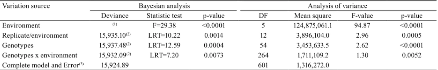
All the variation sources were significant for F and
for the likelihood ratio test (LRT) (Table 1).
As to the assessed environments, two of them were favorable and 4 were unfavorable; the checked
environmental index signal was positive and negative
(Ij). Besides, the coefficient of variation varied from
21.04% up to 51.47% (Table 2).
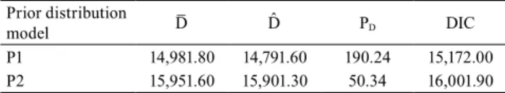
The half-normal was the most appropriate prior
distribution to find the genetic value through MCMC
method. This prior distribution showed the smallest information deviance criterion (DIC), deviance of posterior mean parameters (D̂ ), and deviance of posterior mean (D̅ ), but the effective number of parameters (PD) in positive half-normal was higher than
in the uniform distribution. The larger the effective
number of parameters, the easier the data fit by the
model (Table 3). The half-normal distribution has been used to set the number of replicates in plant breeding experimental designs because it has been showing the smallest deviance criteria (DIC) (Omer et al., 2014b), as well as heritability and genetic gain estimates through the Bayesian approach (Omer et al., 2014a). The DIC is an estimated error prediction; the lower value indicates a better adjusted model. The DIC from half-normal distribution was lower than the distribution uniform value. It indicates that the half-normal prior distribution should be taken into consideration rather than the uniform distribution. Therefore, all the variance components were found through the half-normal prior distribution. Previous experimental data information in genetic experiments lead to better variance estimates and decrease the residual variance (Carneiro Júnior et al., 2005). Moreover, the chosen of priors to calculate posteriors, conducted through the Bayesian approach, was generated according to the inverse variance of 18 genotypes, collected from 55 genotypes in the present study.
The genotype behavior was estimated in percentiles of the previous values, and in their ranks, according
Table 1. Deviance analyses and F-test to measure the random and fixed effects, respectively, on soybean grain yield (kg ha-1).
Variation source Bayesian analysis Analysis of variance
Deviance Statistic test p-value DF Mean square F-value p-value
Environment (1) F=29.38 <0.0001 5 124,875,061.1 94.87 <0.0001
Replicate/environment 15,935.10(2) LRT=10.22 0.0014 12 3,896,104.0 2.96 0.0005
Genotypes 15,937.48(2) LRT=12.59 0.0004 54 3,453,633.5 2.62 <0.0001
Genotypes x environment 15,932.09(2) LRT=7.20 0.0073 264 1,711,109.2 1.30 0.0052
Complete model and Error(3) 15,924.89 601 1,316,272.0
(1)Fixed effect was not calculated. F, F-test calculated; LRT, likelihood ratio test conducted through chi-square at 1 degree of freedom. Chi-square table
value at 1% equals 3.83, and, at 5%, equals 6.63. (2)Adjusted deviance model without the referred effect. (3)Complete model for Bayesian analysis and
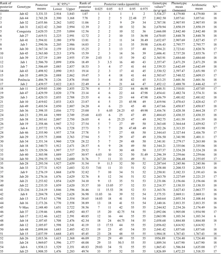
to the posterior mean by using the Bayesian approach (Table 4). Moreover, the mean national soybean grain
yield is 2,870 kg ha-1 (Conab, 2017). Thus, taking into
account the credibility interval, the genotypes Jab 42,
Jab 44, Jab 32, Jab 31, Conquista, Jab 27, Jab 41, and
Jab 5 showed higher values of the limit credibility interval that were above the mean national grain yield; therefore, they were considered the most productive genotypes. Besides, the Jab 42 line remains in the breeding process, and it was herein highlighted as a potential genotype that shows grain yield values above the national mean (Table 4).
Genotypes Jab 48, Jab 15, Jab 26, Jab 24, Jab 6, and Jab 25 did not reach a high rank, taking into
consideration the percentiles 2.5 and 5%; therefore,
they should not be selected. According to the ranks, the
percentiles 95 and 97.5% would show the predictions
of the most unproductive genotypes, if it was selected based on the mean. Genotype Jab 42 may decrease to the 2nd position (percentile 97.5%), or remain in the 1st
one (percentile 95%, and others).
Means obtained through the Bayesian approach, lsmeans, and genotypic mean were the least discrepant ones for magnitude and rank (Tables 4 and 5) because they are methods based on experimental designs used to adjust the means whenever necessary. The posterior distribution in the Bayesian method is generated for the studied parameters (genotype, heritability etc.) as
a random effect. Genotypes are treated as fixed effect
in lsmeans or in marginal mean predictions, and mean adjustment is done according to the factor found in the linear model (genotype, replicate/environment, and environment). Genotypes are treated as random effects in the mixed model method, and the same genotype
mean in multi-environment experiments is equal to the general mean + Blup of the genotype + Blup in GxE
interaction (Resende, 2007).
The Bayesian method and Blups were similar for
correlation means; they recorded r = 0.9974. The
lsmeans method used to calculate the mean genotype showed the second highest correlation values through
the Bayesian method, r = 0.9678. And the simple
arithmetic mean method showed correlation r = 0.9663 (Table 5). The REML/Blup method is the standard one to calculate the random effects on genotype selection in plant breeding (Oliveira et al., 2016). This method showed a high correlation with the Bayesian approach in partially unbalanced experimental situations.
In the present study, there were 5% missed plots, and
the data set was restricted to six plots only. However,
these missed plots did not significantly influence the
genotype rank effect. Thus, it is necessary to assess the Bayesian approach in a larger number of missed plots, environments, and heterogeneous variance situations,
in order to verify its efficiency. The Bayesian approach
was used to model the heterogeneous variances in an experiment conducted to estimate the error and the genotype x environment interaction variances. The Bayesian approach was able to provide a more parsimonious answer to the question about whether the use of weighted, or unweighted means, in multi-environment trial modeling, properly sets the heterogeneous variances in the assessed experiments (Edwards & Jannink, 2006).
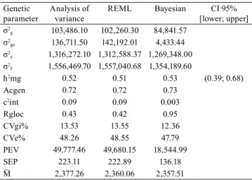
The genetic parameters estimated through the analysis of variance and through the mixed model were similar to all the assessed genetic parameters. The genetic parameters estimated through the
Table 3. Discrepancy statistics to the prior selection in a soybean trial for grain yield (kg ha-1) conducted in six environments.
Prior distribution
model D̅ D̂ PD DIC
P1 14,981.80 14,791.60 190.24 15,172.00 P2 15,951.60 15,901.30 50.34 16,001.90
D̅ , posterior mean of -2 x log-likelihood. D̂, -2 x log-likelihood to pos-terior mean parameters. PD, parameter effective number. DIC, deviance
criteria information. P1, σ2
E, σ2G, σ2R, and σ2GE independent distribution
~ positive half-normal with inverse variance = σ2
E (0, 0,00028), σ2G.(0,
0,00304),σ2
R .(0, 0,00001), and σ2GE .(0, 0,00170). P2, σ2E, σ2G, σ2R, and σ2GE
independent ~ uniform (0, and 5,000,000). Table 2. Soybean grain yield, overall mean, and the
environmental index of the assessed locations and crop seasons.
Location Crop season
Grain yield (kg ha-1)
Coefficient of
variation (%) Environmen-tal index (Ij)
Jaboticabal 2013/2014 1,901.36 44.24 -475.90 Jaboticabal 2014/2015 2,335.26 38.21 -42.00 Jaboticabal 2015/2016 2,169.60 51.47 -207.66 Piracicaba 2013/2014 3,383.12 21.04 1,005.86 Piracicaba 2014/2015 3,371.36 44.51 994.10 Pindorama 2013/2014 1,050.01 31.00 -1,327.25
-Table 4. Genotype mean predicted were ordered by posterior means, and its ranks were measured by the Bayesian approach and the frequentist analyses based on predicted genotypic values (BLUPs), on adjusted mean, and on the arithmetic mean of 55 soybean lines for grain yield (kg ha-1).
Rank of posterior means
Genotype Posterior means
IC 95%(1) Rank of
posterior means
Posterior ranks (quantile) Genotypic values(2)
(u+g+ge)
Phenotypic mean (lsmeans)
Arithmetic mean N(3) Lower Upper 0.025 0.05 0.5 0.95 0.975
1 Jab 42 3,331.33 2,914 3,843 1.07 1 1 1 1 2 3,514.27 4,179.80 4,179.80 18 2 Jab 44 2,743.28 2,390 3,168 7.78 2 2 5 22.48 27 2,802.50 3,057.61 3,057.61 18 3 Jab 32 2,655.86 2,262 3,052 11.06 2 2 9 29 34 2,707.58 2,907.95 2,907.95 18 4 Jab 31 2,622.42 2,260 2,994 12.39 2 2 10 32 36 2,670.94 2,850.19 2,850.19 18 5 Conquista 2,620.53 2,255 3,004 12.56 2 2 10 32 36 2,666.00 2,842.40 2,842.40 18
6 Jab 27 2,619.51 2,225 2,991 12.72 2 2 10 33 36.98 2,670.05 2,848.78 2,848.78 18
7 Jab 41 2,594.81 2,180 2,970 13.81 2 2 11 34 38.49 2,652.07 2,907.69 2,827.45 17 8 Jab 5 2,590.56 2,205 2,986 14.03 2 2 11 35 39.98 2,636.43 2,795.77 2,795.77 18 9 Jab 30 2,567.34 2,159 2,934 15.25 2 3 13 37 40 2,594.21 2,723.61 2,820.76 17 10 Jab 45 2,563.80 2,213 2,976 15.59 2 3 14 36 39 2,606.41 2,737.20 2,835.76 17 11 Jab 39 2,527.19 2,189 2,955 17.39 2.03 3 15 39 42 2,565.91 2,684.60 2,684.60 18 12 Jab 1 2,506.70 2,099 2,856 18.49 3 3.5 16 40 43 2,557.47 2,671.29 2,671.29 18
13 Jab 7 2,506.69 2,085 2,857 18.53 3 4 17 41 44 2,539.33 2,642.69 2,642.69 18
14 Jab 43 2,498.92 2,090 2,913 19.14 2 3 17 41 45 2,530.52 2,597.47 2,651.90 17 15 Jab 35 2,489.26 2,088 2,862 19.47 3 4 18 41 44 2,503.67 2,540.52 2,609.15 17 16 Potência 2,486.78 2,126 2,876 19.60 3 4 18 42 45 2,513.25 2,601.56 2,601.56 18
17 Jab 2 2,439.57 2,022 2,813 22.49 4 5 21 44 47 2,452.12 2,488.70 2,446.42 17 18 Jab 11 2,439.03 2,100 2,855 22.78 4 5 22 44 46.98 2,448.51 2,510.01 2,437.05 17
19 Jab 47 2,429.59 2,020 2,778 23.14 4 6 22 44 47.98 2,454.61 2,482.74 2,574.31 16
20 Jab 3 2,420.53 2,055 2,788 23.55 4 6 23 44 47.98 2,436.79 2,481.02 2,481.02 18 21 Jab 10 2,419.02 2,033 2,821 23.87 4 5 23 45.98 49 2,419.94 2,470.63 2,428.62 17 22 Jab 49 2,410.54 2,050 2,807 24.20 4 6 23 45 48 2,417.66 2,450.87 2,450.87 18 23 Jab 36 2,398.55 2,016 2,772 25.00 5 6.05 24.25 45 49.98 2,416.74 2,420.38 2,464.28 17 24 Jab 23 2,391.44 1,989 2,749 25.68 4.03 6 25 47 49 2,404.65 2,430.35 2,430.35 18 25 Jab 38 2,383.61 2,007 2,750 26.05 4 6 25.25 47 49 2,392.75 2,411.59 2,411.59 18 26 Jab 19 2,358.46 1,947 2,712 27.54 5 7 27 49 50 2,363.68 2,364.64 2,439.82 17
27 Jab 4 2,357.72 1,976 2,728 27.73 5 7 28 47.48 49 2,352.26 2,313.35 2,433.90 17 28 Jab 46 2,355.90 1,957 2,718 27.78 5 7 27 48 50 2,344.65 2,327.44 2,416.70 17 29 Jab 29 2,355.75 2,008 2,763 27.94 5 7 29 47 49 2,356.50 2,341.90 2,401.11 17 30 Jab 34 2,351.34 1,960 2,728 28.22 5 7 29 48 50 2,341.81 2,279.17 2,263.80 16 31 Jab 18 2,340.73 1,912 2,671 28.57 6 9 28 49 50 2,344.21 2,335.06 2,335.06 18 32 Jab 51 2,329.56 1,997 2,717 29.52 7 9 30 48 50 2,337.37 2,324.28 2,324.28 18 33 Jab 40 2,303.98 1,889 2,657 30.97 6.03 10 32 50 51.49 2,296.39 2,259.66 2,259.66 18 34 Jab 50 2,294.55 1,943 2,680 31.76 7 11 33 49 51 2,267.20 2,206.48 2,255.05 17 35 Jab 28 2,293.54 1,927 2,659 31.54 9 11.5 32 50 52 2,287.64 2,245.86 2,245.86 18 36 Jab 33 2,277.31 1,925 2,683 32.53 7.01 11 33 51 52 2,258.88 2,200.53 2,200.53 18
37 Jab 9 2,276.19 1,868 2,670 32.82 7 10 34 51 52 2,250.81 2,182.33 2,191.63 16 38 Jab 20 2,276.16 1,876 2,629 32.76 8 12 34 51 52 2,263.70 2,227.69 2,221.25 17 39 Jab 21 2,253.82 1,854 2,629 34.10 9 13 35 51 53 2,231.06 2,156.66 2,156.66 18 40 Jab 22 2,233.35 1,859 2,620 35.37 10 13.05 37 52 53 2,214.37 2,130.35 2,130.35 18 41 CD-216 2,214.19 1,846 2,596 36.46 11 15.53 38 52 53 2,163.76 2,027.43 2,063.77 16 42 Jab 8 2,204.78 1,842 2,628 36.98 11.03 16 39 52 54 2,175.53 2,069.11 2,069.11 18 43 Jab 13 2,175.63 1,798 2,554 38.65 14.03 18 41 53 54 2,160.64 2,055.34 2,108.44 16 44 Jab 16 2,173.26 1,770 2,558 38.89 13 18 41 53 54 2,140.16 2,013.35 2,013.35 18
45 V-Max 2,148.40 1,651 2,722 38.56 7 11 42 55 55 2,244.82 2,234.26 2,174.49 16
46 Jab 37 2,139.46 1,696 2,492 40.57 15 20 42.75 54 55 2,092.06 1,905.08 1,954.90 17
47 Jab 17 2,112.46 1,622 2,591 40.85 12 16 44 55 55 2,063.98 1,103.34 1,103.34 6
48 Jab 14 2,107.45 1,708 2,476 42.34 18 24 44.75 54 55 2,058.68 1,884.88 1,884.88 18 49 Jab 12 2,105.07 1,598 2,541 41.19 13 17.53 44 55 55 2,056.02 1,614.92 1,614.92 7 50 Jab 48 2,098.04 1,683 2,485 42.53 19 23 45 54 55 2,041.42 1,857.68 1,857.68 18 51 Jab 15 2,037.59 1,668 2,451 45.45 23 28 48 55 55 1,984.18 1,767.43 1,767.43 18 52 Jab 26 2,015.36 1,615 2,368 46.09 25 29 49 55 55 1956.89 1,724.40 1,724.40 18 53 Jab 24 1,969.07 1,596 2,377 48.08 29 33 50.5 55 55 1,889.34 1,617.90 1,617.90 18 54 Jab 6 1,938.13 1,529 2,351 48.83 29.03 34 51 55 55 1,865.43 1,586.84 1,635.00 17 55 Jab 25 1,908.55 1,476 2,283 49.74 33 37 52 55 55 1,826.89 1,472.25 1,518.55 17
(1)Posterior of the credibility interval. (2)Genotypic value: general experimental mean + Blup + GE interaction mean. (3)Total of replicate number by which
Bayesian approach and the mixed model were similar to the heritability at mean level (h2mg), genotype
selection accuracy (Acgen), and genetic variation
coefficient (CVgi%) (Table 6). Besides, the heritability
and genotypic correlation values between genotype behaviors corroborate the published literature if one takes into consideration the different grain yield (kg ha-1) environments (Di Mauro et al., 2014).
Accuracy values were classified as high in both the
Bayesian and mixed model methodologies, as these
methods showed values above 0.7 (Resende & Duarte, 2007).
The Bayesian approach showed the smallest GE interaction variance, showing the lowest determination
coefficient of the GE interaction (c2int). Consequently,
the genotypic correlation coefficient between
genotypes in different environments (rgloc) increased up to the unit value. A rgloc value close to the unit in genotype selection implies a genotype-selection
confidence increase in some tested environments (Resende, 2007).
The GE interaction defined that rgloc ≥ 0.80 in
simulation studies, using the analysis of variance,
indicates a simple interaction. A rgloc ≤ 0.20 evidences
a complex interaction (Cruz & Castoldi, 1991). Thus, rgloc close to one indicates lesser complex GE interaction, adaptability, and stability because of the variation decrease of the environment (Rosado et al., 2012). The interaction effect is associated with two
factors: the first simple one, which is the variability
difference between genotypes in the environments;
and the second one (the complex factor), which is indicated by genotype superiority inconsistency with the environment variation. In other words, there are genotypes that shows a superior behavior in a certain environment, but the same genotype is not observed in another environment; so, it increases intricacy in the suggested selection (Cruz et al., 2012).
The predicted error variance (PEV) in genotype
values and the standard deviation in genotypic variance values (SEP) in the Bayesian approach were smaller than those in the mixed model, indicating a better adjustment in the mean soybean genotype calculated a posteriori. The smaller PEC and SEP values are desirable for plant breeding programs because they are directly linked to precision and accuracy maximization
(Resende & Suarte, 2007).
The advantages of using the Bayesian method in experimental data lies on its methodology, which
Table 5. Correlation coefficient between means and ranks of all the assessed methods. Superior diagonal, Pearson correlation between mean genotypes and the inferior diagonal, Spearman correlation coefficient between genotype ranks for soybean grain yield (kg ha-1).
Bayesian Blups Lsmeans Arithmetic Bayesian
- 0.99742 0.96775 0.96627 <0.0001* <0.0001 <0.0001 Blups 0.99740
- 0.97256 0.96945 <0.0001 <0.0001 <0.0001 Lsmeans 0.98954 0.99430
- 0.99629
<0.0001 <0.0001 <0.0001 Arithmetic 0.98867 0.99091 0.99019
-<0.0001 <0.0001 <0.0001
*Significant by the t-test at 5% probability.
Table 6. Genetic parameters estimated through the analysis of variance, likelihood method, and Bayesian approach for soybean grain yield (kg ha-1).
Genetic parameter
Analysis of variance
REML Bayesian CI 95% [lower; upper] σ2
g 103,486.10 102,260.30 84,841.57
σ2
ge 136,711.50 142,192.01 4,433.44
σ2
e 1,316,272.10 1,312,588.37 1,269,348.00
σ2
f 1,556,469.70 1,557,040.68 1,354,189.60
h2mg 0.52 0.51 0.53 (0.39; 0.68)
Acgen 0.72 0.72 0.73
c2int 0.09 0.09 0.003
Rgloc 0.43 0.42 0.95
CVgi% 13.53 13.55 12.36
CVe% 48.26 48.55 47.79
PEV 49,777.46 49,680.15 18,544.99
SEP 223.11 222.89 136.18
M̅ 2,377.26 2,360.06 2,357.51
σ σ σ σ
f g ge e 2= 2+ 2 + 2
,phenotypic variance; σ2
g, genotypic variance; σ2ge,
genotypic x environment interaction variance; c ge f 2int= σ2 σ2, de-termination coefficient of the GE interaction effect; σ2
e, residual
va-riance; h mg g g ge N env g N env N rep
2 2 2 2 2
=σ
(
σ +σ . +σ ( . × . ))
is the heritability at mean level (genotype); Acgen=(
1−PEV g)
2
σ is the genotype selection accuracy; CVgi= σg M
2 is the genetic coefficient
variation; CVe= σe2 M is the environmental variation coefficient;
rgloc=σg
(
σg+σge)
2 2 2 is the genotypic correlation between genotype
behavior in several environments; PEV Acgen
g =
(
1− 2)
× 2allows of the use of previous data information, presents a lesser sensitive modeling to outliers than the frequentist methods, and works well with lesser assumptions (large sample numbers, balance experiments, etc.) in analysis processes (Singh et al., 2015).
It is worth highlighting that the Bayesian approach applied to complex agriculture experimental data, such as years, crops, location, and interaction in the model, takes a bit longer than the mixed model in
computer processes. Besides, with regard to specific
cases based on prior information, the Bayesian analysis could assemble a posterior distribution, which would
be highly influenced by the prior information. In this
case, it is recommended to use the prior information as parsimony (Gelman, 2006).
Conclusions
1. The mixed models and the Bayesian methodology show similar genetic parameters.
2. The mean genotypic values obtained through the Bayesian approach differ from those obtained through the frequentist method.
3. The Bayesian approach uses previous soybean experimental data information that can be used as tools in soybean breeding programs.
Acknowledgments
To Coordenação de Aperfeiçoamento de Pessoal de Nível Superior (Capes), for a doctoral scholarship to
the first author.
References
BORGES, V.; FERREIRA, P.V.; SOARES, L.; SANTOS, G.M.;
SANTOS, A.M.M. Seleção de clones de batata-doce pelo procedimento REML/BLUP. Acta Scientiarum. Agronomy,
v.32, p.643-649, 2010. DOI: 10.4025/actasciagron.v32i4.4837.
CARNEIRO JÚNIOR, J.M.; ASSIS, G.M.L. de; EUCLYDES,
R.F.; LOPES, P.S. Influência da informação a priori na avaliação
genética animal utilizando dados simulados. Revista Brasileira de Zootecnia, v.34, p.1905-1913, 2005. DOI: 10.1590/S1516-35982005000600014.
CONAB (Brasil). Séries históricas de área plantada, produtividade e produção. 2017. Available at: <https://
por t aldei nfor macoes.conab.gov.br/i ndex.php/saf ra-ser
ie-historica-dashboard>. Accessed on: Mar. 5 2017.
CRUZ, C.D.; CASTOLDI, F.L. Decomposição da interação genótipos x ambientes em partes simples e complexa. Revista Ceres, v.38, p.422-430, 1991. Available at: <http://www.ceres.ufv. br/ojs/index.php/ceres/article/view/2165/203>. Accessed on: Oct. 12 2016.
CRUZ, C.D.; REGAZZI, A.J.; CARNEIRO, P.C.S. Modelos biométricos aplicados ao melhoramento genético. 4.ed. Viçosa:
Ed. da UFV, 2012. v.1, 514p.
DI MAURO, A.O.; GOMEZ, G.M.; UNÊDA-TREVISOLI,
S.H.; PINHEIRO, J.B. Adaptive and agronomic performances of soybean genotypes derived from different genealogies through the use of several analytical strategies. African Journal of Agricultural Research, v.9, p.2146-2157, 2014. DOI: 10.5897/
AJAR2014.8700.
EDWARDS, J.W.; JANNINK, J.-L. Bayesian modeling of heterogeneous error and genotype x environment interaction variances. Crop Science, v.46, p.820-833, 2006. DOI: 10.2135/ cropsci2005.0164.
GELMAN, A. Prior distributions for variance parameters in hierarchical models (comment on article by Browne and Draper). Bayesian Analysis, v.1, p.515-534, 2006. DOI:
10.1214/06-BA117A.
GELMAN, A.; RUBIN, D.B. Inference from iterative simulation using multiple sequences. Statistical Science, v.7, p.457-472,
1992. DOI: 10.1214/ss/1177011136.
OLIVEIRA, G.H.F.; BUZINARO, R.; REVOLTI, L.T.M.;
GIORGENON, C.H.B.; CHARNAI, K.; RESENDE, D.; MORO,
G.V. An accurate prediction of maize crosses using diallel analysis
and best linear unbiased predictor (BLUP). Chilean Journal of Agricultural Research, v.76, p.294-299, 2016. DOI: 10.4067/
S0718-58392016000300005.
OMER, S.O.; ABDALLA, A.W.H.; CECCARELLI, S.; GRANDO, S.; SINGH, M. Bayesian estimation of heritability and genetic gain for subsets of genotypes evaluated in a larger set of genotypes in a block design. European Journal of Experimental Biology, v.4, p.566-575, 2014a.
OMER, S.O.; ABDALLA, A.W.H.; MOHAMMED, M.H.; SINGH, M. Bayesian estimation of genotype-by-environment interaction in sorghum variety trials. Communications in Biometry and Crop Science, v.10, p.82-95, 2015.
OMER, S.O.; ABDALLA, A.W.H.; SARKER, A.; SINGH, M. Bayesian determination of the number of replications in crop trials. European Journal of Experimental Biology, v.4, p.129-133, 2014b.
PRIOLLI, R.H.G.; WYSMIERSKI, P.T.; CUNHA, C.P. da;
PINHEIRO, J.B.; VELLO, N.A. Genetic structure and a
selected core set of Brazilian soybean cultivars. Genetics and Molecular Biology, v.36, p.382-390, 2013. DOI:
10.1590/S1415-47572013005000034.
R CORE TEAM. R: the R project for statistical computing.
RESENDE, M.D.V. de. SELEGEN-REML/BLUP: sistema estatístico e seleção genética computadorizada via modelos
lineares mistos. Colombo: Embrapa Florestas, 2007. 359p. RESENDE, M.D.V. de; DUARTE, J.B. Precisão e controle de
qualidade em experimentos de avaliação de cultivares. Pesquisa Agropecuária Tropical, v.37, p.182-194, 2007.
ROSADO, A.M.; ROSADO, T.B.; ALVES, A.A.; LAVIOLA,
B.G.; BHERING, L.L. Seleção simultânea de clones de eucalipto de acordo com produtividade, estabilidade e adaptabilidade.
Pesquisa Agropecuária Brasileira, v.47, p.964-971, 2012. DOI:
10.1590/S0100-204X2012000700013.
SHEN, Y.; LIU, X. Phenological changes of corn and soybeans over US by Bayesian change-point model. Sustainability, v.7,
p.6781-6803, 2015. DOI: 10.3390/su7066781.
SINGH, M.; AL-YASSIN, A.; OMER, S.O. Bayesian estimation of genotypes means, precision, and genetic gain due to selection from routinely used barley trials. Crop Science, v.55, p.501-513, 2015. DOI: 10.2135/cropsci2014.02.0111.
SPIEGELHALTER, D.J.; BEST, N.G.; CARLIN, B.P.; VAN DER LINDE, A. Bayesian measures of model complexity and fit.
Journal of the Royal Statistical Society: Series B (Statistical
Methodology), v.64, p.583-639, 2002. DOI:
10.1111/1467-9868.00353.
STURTZ, S.; LIGGES, U.; GELMAN, A. R2WinBUGS: a package for running WinBUGS from R. Journal of Statistical Software, v.12, p.1-16, 2005. DOI: 10.18637/jss.v012.i03.
VALENTIM, F.L.; SILVA, R.M.D.A.; ALVES, M.D.C. Modelos
de redes bayesiana para incidência da ferrugem asiática na soja, cultivar Suprema, em diferentes condições de temperatura e molhamento foliar. In: SIMPÓSIO BRASILEIRO DE PESQUISA
OPERACIONAL, 39., 2007, Fortaleza. A pesquisa operacional e
o desenvolvimento sustentável: anais. Fortaleza: [s.n.], 2007. p.
2677-2678.
ZEILEIS, A.; HOTHORN, T. Diagnostic checking in regression relationships. R News, v.2/3, p.7-10, 2002. Available at: <http://
CRAN.R-project.org/doc/Rnews/>. Accessed on: Oct. 19 2016.