McSCIA: application of the Equivalence Theorem in a Monte Carlo radiative transfer model for spherical shell atmospheres

(1)

ACPD

6, 1199–1248, 2006

McSCIA: Monte Carlo Equivalence Theorem

Radiative Transfer model

F. Spada et al.

Title Page Abstract Introduction Conclusions References Tables Figures

◭ ◮

Back Close Full Screen / Esc

Print Version

Interactive Discussion

EGU Atmos. Chem. Phys. Discuss., 6, 1199–1248, 2006

www.atmos-chem-phys.org/acpd/6/1199/ SRef-ID: 1680-7375/acpd/2006-6-1199 European Geosciences Union

Atmospheric Chemistry and Physics Discussions

McSCIA: application of the Equivalence

Theorem in a Monte Carlo radiative

transfer model for spherical shell

atmospheres

F. Spada1, M. C. Krol1,2,3, and P. Stammes4

1

Institute for Marine and Atmospheric Research (IMAU), Utrecht University, The Netherlands

2

Earth Oriented Science (EOS), Netherlands Institute for Space Research (SRON), Utrecht, The Netherlands

3

Meteorology and Air Quality, Wageningen University, The Netherlands

4

Climate Research and Seismology, Royal Netherlands Meteorological Institute (KNMI), De Bilt, The Netherlands

Received: 10 November 2005 – Accepted: 20 December 2005 – Published: 15 February 2006 Correspondence to: F. Spada (f.spada@phys.uu.nl)

(2)

ACPD

6, 1199–1248, 2006

F. Spada et al.

◭ ◮

Print Version

EGU

Abstract

A new multiple-scattering Monte Carlo 3-D radiative transfer model named McSCIA (Monte Carlo for SCIAmachy) is presented. The backward technique is used to ef-ficiently simulate narrow field of view instruments. The McSCIA algorithm has been formulated as a function of the Earth’s radius, and can thus perform simulations for

5

both plane-parallel and spherical atmospheres. The latter geometry is essential for the interpretation of limb satellite measurements, as performed by SCIAMACHY on board of ESA’s Envisat. The model can simulate UV-vis-NIR radiation.

First the ray-tracing algorithm is presented in detail, and then successfully validated against literature references, both in plane-parallel and in spherical geometry. A

sim-10

ple 1-D model is used to explain two diff_{erent ways of treating absorption. One method}

uses the single scattering albedo while the other uses the equivalence theorem. The equivalence theorem is based on a separation of absorption and scattering. It is shown that both methods give, in a statistical way, identical results for a wide variety of sce-narios. Both absorption methods are included in McSCIA, and it is shown that also

15

for a 3-D case both formulations give identical results. McSCIA limb profiles for atmo-spheres with and without absorption compare well with the one of the state of the art Monte Carlo radiative transfer model MCC++_.

A simplification of the photon statistics may lead to very fast calculations of absorp-tion features in the atmosphere. However, these simplificaabsorp-tions potentially introduce

20

(3)

ACPD

6, 1199–1248, 2006

F. Spada et al.

◭ ◮

Print Version

EGU

1. Introduction

In recent years the chemical composition of the atmosphere has become an important concern (e.g.Jacob,1999). Due to human activities the composition of the atmosphere is changing, not only on a local scale, but also on a global scale. Many of these changes are related to trace gases present in the atmosphere (e.g. O3, NO2, CO2). To

5

increase our knowledge on sources and sinks of these trace gases long time series of measurements are needed on a global scale, which can not be provided by ground stations only. Therefore, there has recently been an increase in new satellites with new instruments and capabilities. The aim of these new instruments is to monitor our changing atmosphere and understand, in synergy with chemical models and ground

10

observations, the mechanisms behind the changes in atmospheric composition. Many satellite instruments are designed to sample the atmospheric composition us-ing the UV-vis-NIR part of the spectrum. Employus-ing the gas absorption spectral fea-tures it is possible to retrieve the total column gas concentration of O3, NO2, SO2, CO, CH4, CO2from the backscattered solar radiation. Using the backscattered UV-vis-NIR

15

solar radiation, for instance, GOME on board of ESA’s ERS-2 (Burrows et al.,1999) employs a diff_{erential optical absorption spectroscopy (DOAS) method to obtain global}

distributions of various trace gases. Also the more recent instruments SCIAMACHY (Bovensmann et al.,1999) (launched 1 March 2002 onboard of ESA’s Envisat), and OMI (Levelt et al.,2005; Stammes et al., 1999) (launched 15 July 2004 on board of

20

NASA’s EOS-Aura) use DOAS-like techniques to retrieve trace gas concentrations. Whereas GOME and OMI are nadir viewing instruments, SCIAMACHY scans the atmosphere also in limb mode, giving the possibility to obtain stratospheric profiles and consequently tropospheric trace gas columns.

The limb view enables the retrieval of vertical profiles of trace gases (see e.g.Rusch

25

et al.,1984;Mount et al.,1984;Flittner et al.,2000;Kaiser,2002;von Savigny et al.,

(4)

ACPD

6, 1199–1248, 2006

F. Spada et al.

◭ ◮

Print Version

EGU plane-parallel description of the atmosphere normally suffi_{ces, in limb it is essential to}

consider the sphericity of the Earth. One approach to solve this problem is the use of a Monte Carlo (MC) RT model (Oikarinen et al.,1999). Monte Carlo methods are in principle an accurate way of solving RT problems, and are often used as a benchmark for approximate approaches (e.g. Walter and Landgraf, 2005). All other approaches

5

work with some assumption to solve the RT equation in spherical geometry (see

Leno-ble,1985;Marshak and Davis,2005, for a review of diff_{erent methods). Despite the}

fact that a Monte Carlo approach can be very time consuming, it also gives statisti-cal information that allows to evaluate the error of the results. Another advantage that will be explored in this paper is the possibility to separate scattering from absorption.

10

The separate treatment of these processes is achieved using the Equivalence Theo-rem (ET). Although it was already introduced byIrvine(1964) and illustrated byvan de

Hulst (1980), only recently a rigourous implementation, also for nontrivial cases, was published (Partain et al.,2000). In short, the ET states that it does not matter whether the constituents doing the scattering and doing the absorption are identical, i.e.

ab-15

sorption can be treated as only happening at the scattering points or only along the photon paths. In previous works on ET (van de Hulst,1980;Feigelson,1984;Cahalan

et al., 1994;Partain et al.,2000) normalised probability distribution functions (PDFs) of photons paths were derived, using Monte Carlo models. These PDFs were used to calculate the absorption in the atmosphere. In the studies of the radiation in a cloudy

20

atmosphere presented byFeigelson(1984), she proposes instead to derive equivalent trajectories that can be convoluted with absorption profiles of gases. Since this ap-proach is only valid in the weak absorption limit, this kind of treatment of absorption introduces a new approximation that we would like to avoid.

The purpose of this work is to introduce the MC RT model named McSCIA and to

25

illustrate the use of the ET. For the first time we will show that the ET and the single scattering approach (SSA) give identical results in a 3-D spherical RT model, both in nadir and limb geometry.

(5)

ACPD

6, 1199–1248, 2006

F. Spada et al.

◭ ◮

Print Version

EGU perform a validation (Sect.3) of this module. We will introduce absorption in Sect.4

and illustrate the two approaches that we will exploit in the paper: the SSA and the ET. After a theoretical illustration on how to apply absorption in a MC model (Sect. 4.1), we will use a simple 1-D model, in Sect. 4.2, to introduce the reader to a MC RT model with absorption. We will show that the SSA and the ET approach give identical

5

results in 1-D. The validation of the 3-D implementation of McSCIA against the state-of-the-art MC RT model MCC++₍_Postylyakov_,₂₀₀₄_{) will be done in Sect.}₅_{, where we}

will show that the SSA and ET approach give statistically the same results in a wide variety of scenarios. After a discussion in Sect.6on the earlier use of the ET and the comparison with our approach, we will summarise in Sect.7our results and draw some

10

conclusions.

2. McSCIA ray-tracing algorithm

McSCIA is a scalar (no polarisation) backward (or time-reversed, or adjoint) MC RT model, in which photons are tracked from their starting position in the satellite, until the end their trajectories in space. The implementation is similar to SIRO (Oikarinen

15

et al.,1999), but the refractive bending is not implemented. The basis of MC (see also

Cashwell and Everett,1959;Spanier and Gelbard,1969;Lenoble,1985;Marshak and

Davis,2005) is that every interaction of a photon in the atmosphere can be described via a probability density function (PDF), the integral of which can be linked to a random number R (see the Appendix for some examples). By generating enough random

20

realisations, the physical process can be simulated in a statistical sense. Once the probability of one event is known, it is possible to calculate the probability of a sequence of events as a Markov chain, because the events are independent.

However, there is a drawback in this approach. Every result of a MC model has a statistical noise, and the accuracy depends on the number of realisations. The more

25

(6)

ACPD

6, 1199–1248, 2006

F. Spada et al.

◭ ◮

Print Version

EGU Since the field of view (FOV) of the satellite is normally narrow usually a backward

MC approach is preferred (Collins et al., 1972;Adams and Kattawar,1978; Marchuk

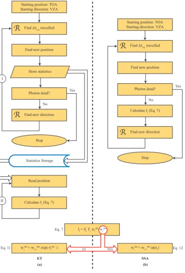
et al.,1980;Lenoble,1985;Oikarinen et al.,1999). The principle behind this method is illustrated in Fig.1. With a time reversal, photons emerge from the detector and are traced through the atmosphere. The fate of these photons is influenced by scattering

5

on air molecules (Rayleigh), aerosols (Mie), absorption by trace gases, and surface reflection. Since in the UV-vis wavelength region emission can be generally ignored, the only source of light is the sun. However, the chance that a photon leaves the at-mosphere exactly in the direction of the sun are extremely low. Thus, many photons would be needed to obtain a statistically meaningful result. Luckily a much faster

con-10

vergence can be obtained by using the local estimate technique (Marchuk et al.,1980;

Davis et al., 1985;Marshak and Davis, 2005). It consists in calculating the contribu-tion of every photon at each scattering event (see Fig.1). If we follow thejth photon (e.g. the one of Fig.1), at each scattering positionx_i, the probabilities that the photons

escape in the direction of the sun are calculated. For a scattering-only atmosphere the

15

radiance contribution of this photon at the i-th scattering event is given by

I_i =_S_i ·T_i. (1)

S_i is the scattering probability towards the sun

Si =P(µsi)/4π, (2)

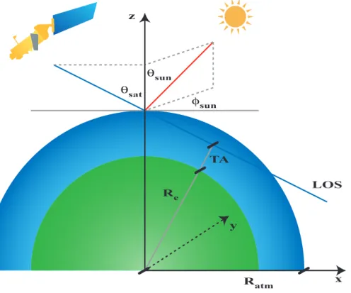
whereµsi is the cosine of the scattering angle towards the sun, θsi (see also Fig. 1,

20

Eqs.43and44). P(µ) is the scattering phase function, normalised over the solid angle:

Z

4π P(µ)

4π dΩ =1

where dΩ_{is the infinitesimal element of a solid angle, d}Ω=_d_µ_d_φ_{. The transmittance}_T

i in Eq. (1) from the photon position to the TOA in the direction of the sun, which takes into account the intensity scattered out of the ray, is given by:

25

Ti =e

−τ_scai

(7)

ACPD

6, 1199–1248, 2006

F. Spada et al.

◭ ◮

Print Version

EGU whereτsca_i is the outgoing optical thickness:

τ_sca i =

Z

s

k_sca(s)ds. (4)

wheresis the line connecting the scattering positionx

i tox out

i , the position where the photon leaves the atmosphere towards the sun.k_scais the scattering coeffi_cient.

The result of this ray-tracing procedure is a number of scattering positions (x_i, i=1,5

5

in Fig. 1) of all the photons that travel through the model atmosphere. To find the new positions and directions of the photons after each scattering event, we use the formulae described in the Appendix, following the algorithm illustrated by the flow chart of Fig.2a. For the first scattering event in limb geometry we use the biased Eq. (26) instead of Eq. (25). In this way all photons remain in the atmosphere after the first

10

scattering and no photon is lost directly to space. Not using this biasing (Marchuk

et al.,1980) would result in very bad statistics for the limb case.

The photons can only end their trajectories if they are scattered into space.

The normalised radianceI measured by the satellite is given by the sum of all con-tributions at the scattering eventsi of photonj, divided by the total number of photons

15

simulated (Ntot) multiplied byπ

I= π

Ntot N_tot

X

j=1 N_sca(j)

X

i=1

Ii,j. (5)

The number of scattering events that a photon undergoes, Nsca(j), can be different for each photon. The factor π in equation above is needed if we assume that the monochromatic incident solar flux through a surface unit perpendicular to the incident

20

solar beam isπWm−2. Thus the normalised radiance is expressed in sr−1. To obtain the actual value of the radiance, one must multiply it by the extraterrestrial solar spectral irradiance.

(8)

ACPD

6, 1199–1248, 2006

F. Spada et al.

◭ ◮

Print Version

EGU contribution given by the first scattering event of a photon is considered. I_SS is given

by

ISS = π Ntot

N_tot

X

j=1

I1,j. (6)

In addition toI_SS we will refer to the radiance given by total scattering (TS) simply as radianceI orIT S. We choose this terminology, because for the widely used term

mul-5

tiple scattering (MS) it is not always clear if it refers to the total scattering (MS=_TS)

or only to the part that is scattered more than once (MS=_{TS–SS). The SS}

compo-nent, when calculated for nadir with ground albedo greater than zero, will contain the radiation scattered only once by the ground or the atmosphere.

The whole ray-tracing algorithm has been formulated as a function of the Earth’s

10

radiusRearth. This enables McSCIA to increase the Earth’s radius to very large values, eff_{ectively resulting in a plane-parallel atmospheric model. In this way a validation of}

the backward MC algorithm with plane-parallel RTMs is a straightforward exercise.

3. Scattering in a spherical atmosphere: validation of ray-tracing module

The current implementation of the model atmosphere consists of an arbitrary number of

15

homogeneous spherical shells. The depth of each layer is specified independently. The model can treat molecular scattering (Rayleigh phase function, see Eq.29) and aerosol and droplet scattering (Henyey-Greenstein phase function with asymmetry parameter 0≤g≤1, see Eq.33). Since absorption is treated later (see Sect.4), here it is assumed that the atmosphere is conservatively scattering, so the single scattering albedo (SSA),

20

ω, is set to one. The ground reflection is assumed Lambertian, and the ground albedo can have a 2-D variability (see Sect.1). Since absorption will be considered in Sect.4, surface reflection is assumed, just for now, to be conservative. The changes in the model formulation to account for surface or atmospheric absorption are explained in Sect.4.

(9)

ACPD

6, 1199–1248, 2006

F. Spada et al.

◭ ◮

Print Version

EGU Since the algorithm is formulated as a function of Earth radius, the first validation of

the ray-tracing was performed by increasing the radius of McSCIA to 1000·Rearth and comparing our results with the Doubling and Adding model of the KNMI (de Haan et al.,

1987;Stammes,2001), a plane-parallel RT model. The comparison was satisfactory, giving results with diff_{erences less than the statistical error of McSCIA.}

5

Next, as inOikarinen et al. (1999), we compared McSCIA results with results from

Adams and Kattawar(1978) andKattawar and Adams(1978) to verify the implemen-tation of the spherical geometry. For the comparison, the Earth radius was set to 6371 km, and the atmosphere was considered as a homogeneous spherical shell with a height of 100 km. The atmosphere was assumed to be conservatively scattering and

10

the ground albedo was set to zero. In this case the photons end its trajectory when they touch the Earth’s surface. The satellite viewing zenith angleθsatat TOA was varied be-tween 0 and 88◦ in the principal plane. This plane is defined by the relative azimuth angle valuesφ=_φ_sun−φsat=0

◦

orφ=_φ_sun−φsat=180

◦

,φsat is assumed to be 0. In the first case the setup looks like the one in Fig.3, while in the latter the sun is in the left

15

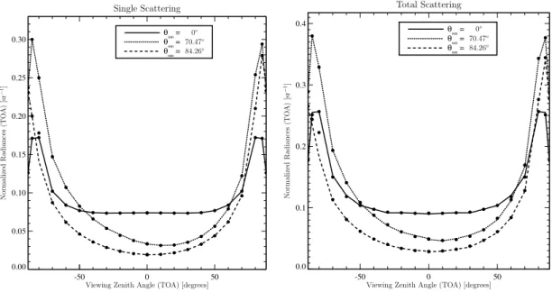
quadrant behind the satellite. As inAdams and Kattawar(1978), five values have been chosen for the solar zenith angleθsunand azimuth angleφsun(see Table1and Fig.4). As an example of the comparison we show the results for two Rayleigh scattering at-mospheres of optical thickness 0.25. In the top panel of Fig.5we show the normalised single scattering (SS) radiance values, while in the bottom panel the normalised

mul-20

tiple scattering (TS) radiance values at top of atmosphere (TOA) for all the three solar positions.

The results of our simulations agree very well with the radiance values obtained by Adams and Kattawar (1978). In most cases results agree to the last digit given in the papers. Otherwise diff_{erences are normally smaller than 1%. In some cases}

25

diff_{erences amount to 3–5%. Since in the original papers there is no indication of the}

statistical error or of the number of photons used, the diff_{erences can be due to poorer}

statistics of the old models.

(10)

ACPD

6, 1199–1248, 2006

F. Spada et al.

◭ ◮

Print Version

EGU thickness of 0.25. First of all, the dotted and dashed curves are not symmetric due

to the solar position, that is not on nadir. For the case in which the solar zenith an-gle is 84.26◦the incoming solar radiation doesn’t intersect the earth anymore, and the satellite can see also some part of ground beyond the terminator. This eff_{ect increases}

the diff_{erence between the radiance values for}_φ=₀◦ _and_φ=₁₈₀◦_{. Another important}

5

feature that McSCIA reproduces is that the radiance values increase until 80◦ and de-crease for greater angles. This feature it is characteristic of the spherical geometry: in this scenario after 80◦ a plane-parallel model would have only a monotonous increase of the radiance for increasing VZA (seeAdams and Kattawar,1978).

These findings are also similar to those obtained by the SIRO model (Oikarinen et al.,

10

1999). Therefore, we are confident that our spherical implementation is correct.

4. Absorption: Equivalence Theorem and Single Scattering Albedo

The Equivalence Theorem (ET) ofIrvine(1964) is a powerful way to include absorption in RT models. As discussed by van de Hulst (1980), the ET states that it does not matter whether the constituents doing the scattering and those doing absorption are

15

identical. This means that if we distinguish two atmospheric constituents

– haze, that causes conservative scattering,

– gas, that causes absorption along the path between scattering points; we can decide to treat absorption as if it would occur

1. only at the scattering points, using a single scattering albedo (ω) of the haze

20

particles less than one, or

2. only along the path between scattering points with conservative scattering, using an exponential decrease of the radianceI along the trajectory following Lambert-Beers law.

From now on we will call case 1 the SSA approach, and case 2 the ET approach.

(11)

ACPD

6, 1199–1248, 2006

F. Spada et al.

◭ ◮

Print Version

EGU 4.1. McSCIA in a 3-D spherical atmosphere with absorption

In the book ofvan de Hulst (1980), it is spelled out how to use the ET for one layer, while in the work ofFeigelson (1984) andPartain et al.(2000) possible uses of it for a multilayer geometry are explored. Partain goes as far as applying it to a case with a vertical profile of an absorbing trace gas. However, these applications are not suitable

5

for a full 3-D study case. So we decided to explore a solution that could work in this case, as proposed, but not used, by O’Hirok and Gautier (1998). Nevertheless, the current implementation of the model is still bounded to as spherical shell atmosphere. In McSCIA the atmosphere is formed by homogeneous spherical shell layers defined by the scattering coeffi_cient _k_sca_{, the absorption coe}ffi_cient _k_abs_{, the phase function}

10

P(µ) and the geometrical extension of each layer.

Using the ET approach (see the flowchart Fig.2a), we perform a simulation of the model in a scattering-only atmosphere with ground albedo equal to 1, as described in Sect.2, and we store all the scattering and ground reflection positions. Once this scattering-only case has been computed, the contribution of each scattering event to

15

the radiance can be evaluated, using a combination of the local estimate and weight techniques (e.g. see Marchuk et al., 1980; Davis et al., 1985; Marshak and Davis,

2005). If we follow only the jth photon, similar to Eq. (1), the value for the i-th event is given by:

I_i =_S_i ·T_i ·w_ialb·w_iabs (7)

20

whereS_i is the scattering probability towards the sun defined in Eq. (2). The other quantities are defined below.

The transmittance from the photon position to the sun is

T_i =_e−τexti ₍₈₎

whereτ_ext

i is the optical thickness travelled by the photon from its current position to

(12)

ACPD

6, 1199–1248, 2006

F. Spada et al.

◭ ◮

Print Version

EGU the sun, calculated integratingkextalong the photon paths

τext_i =

Z

s

kext(s)ds=

Z

s

(ksca(s)+kabs(s)) ds. (9) The diff_{erence between Eq. (}₈_{) and Eq. (}₃_{) is that now also absorption is included in}

the transmission, as can be seen by the diff_{erence between Eq. (}₉_{) and Eq. (}₄_{). In the}

ET method this factor is calculated off_{-line, after the ray-tracing.}

5

To account for a surface albedo less than unity, the weight due to surface reflections, w_ialb, is the cumulative ground albedo at positionx

i

w_ialb=

i

Y

k=1

α(x_k). (10)

The coeffi_cient _α₍x

k)=1 if xk is in the atmosphere, and α(xk)=a(xk) if xk is on the Earth surface, witha(x

k) the ground albedo at pointxk. With this approach the effects

10

of a 2-D variable ground albedo can be easily evaluated.

The cumulative atmospheric absorption weight,w_iabs, is the product of the transmis-sion function from point to point

w_iabs= Y

k=_1,i

e−τabsk_. ₍₁₁₎

whereτabs_k=

R

skabs(s)dsandsis the line connectingxk−1andxk.

15

In the ET approach the atmospheric absorption is accounted for in calculating the extinction from the scattering position towards the sun (Eqs.8,9) and from scattering point to scattering point (Eq.11). Both these factors are calculated off_-line.

If we use, instead, the SSA algorithm to account for absorption, we follow the flowchart of Fig.2b. Now the scattering of the photons is calculated in a scattering and absorbing

20

(13)

ACPD

6, 1199–1248, 2006

F. Spada et al.

◭ ◮

Print Version

EGU Eq. (7), but this time the absorption termw_iabsis given by

w_iabs= Y

k=1,i ω(x

k). (12)

Inspecting the flowcharts of Fig.2it is easy to see that the absorption is calculated “off_{-line” for the ET method (a), while it is calculated “on-line” for the SSA case (b).}

Thus, it is clear that the results of the SSA simulations cannot be re-used if we change

5

the absorption properties of the atmosphere. We should in this case also re-calculate all the scattering positions, since they depend on the absorption coeffi_{cients in the 3-D}

atmosphere. However, the ET calculation with a scattering-only atmosphere can be applied to any distribution of absorbers, as long as the scattering properties remain unchanged.

10

Now that the diff_{erences between the two approaches of calculating absorption have}

been spelled out, we will show that they give equivalent results with a simple 1-D MC RT model.

4.2. Simple 1-D demonstration of the Equivalence Theorem

To demonstrate the use of the ET we have developed a simple one-dimensional MCRT

15

model. The only aim of this model is to illustrate the ET, and would be ideal as a classroom example for RT.

The atmosphere is plane-parallel (PP), and stretches from the ground to 100 km in height. The phase function that we choose is a fully backscattering one, i.e. it inverts the direction of the photon at each scattering event. Therefore, the photons move

20

(14)

ACPD

6, 1199–1248, 2006

F. Spada et al.

◭ ◮

Print Version

EGU scattering coeffi_{cients and single scattering albedo}

k_sca(z)=_c_s_exp−_zz scale

,

kabs(z)=caexp

−(z−zmax)2 2d2

,

ω(z) = ksca k_sca+_k

abs

(13)

wherec_a [km−1], c_s [km−1],d [km], zscale [km], zmax [km] are parameters specified in Table2 and z [km] is the vertical coordinate. The absorption layer formulated in this way, mimics the absorption of UV in the “ozone” layer.

5

In this simple model the weight of the photon (Eq. 11 for ET and Eq. 12 for SSA) is reduced to describe absorption. The ground is supposed to have albedo 0, so the photons end their trajectories either when they hit the ground or as they leave the atmosphere.

In the ET method, the scattering optical depth is used as the vertical coordinate

10

τsca(z)=

Zz_TOA

z

ks(z′)dz′ (14)

wherezTOAis the coordinate of the TOA. The photon is initialised at the TOA in a down-ward direction and its weight is initialized to 1. The new position is calculated using the Eq. (24). If the photon is still in the atmosphere its weight (Eq.11) is calculated. The process starts with an ensemble of photons (e.g. 106) and iterates until all photons

15

leaves the atmospheres. In the case the photon would end its trajectory, on the ground or in space, the weight of the photon contributes to the measured flux at the boundaries of the domain.

Instead, if the SSA approach is used, the total optical depth is used as vertical coor-dinate:

20

τext(z)=

Zz_TOA

z

(kabs(z

′

(15)

ACPD

6, 1199–1248, 2006

F. Spada et al.

◭ ◮

Print Version

EGU It is important to realise that from a numerical point of view a completely diff_erent

atmosphere is simulated: it is optically thicker in the SSA case than in the ET case. Another diff_{erence between the two methods is the way in which the weight is}

calcu-lated: in the ET case the weight due to absorption is exp(−∆_τ_abs_{), where}∆_τ_abs _{is the}

absorption optical thickness between two subsequent scattering events. In the SSA

5

approach, the single scattering albedo evaluated at the scattering position is used to reduce the photon weight.

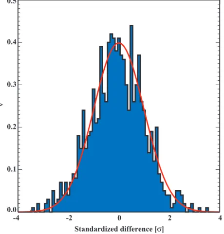
To compare the level of agreement between the two methods many scenarios were simulated (see Table2and Fig.6). The basic scenario was that of Rayleigh scattering with an ozone-like absorber. The absorption peak altitude was alwayszmax=22 km.

10

In each of these scenarios, the amount of absorption was varied in depth (d) and absorption peak value (c_a) (see Table 2) giving more that three thousand diff_erent

scenarios, with absorption optical thickness ranging from 0 to 7.4 and scattering optical depth ranging from 0.08 to 8.0.

To evaluate the statistical error (σ) 10 simulations, each with 105 photons, were

15

performed. The average of these 10 intensities represents the radiance and the sample standard deviation is used to estimate the spread of the radiance. The error is, thus, calculated via the formula

err =_σ/I·100 [%]. (16)

Then, the results of the ET (I1±σ1) and SSA (I2±σ2) cases were compared calculating

20

the standardised diff_{erence (SD) between the two models}

SD= I1−I2

q

σ₁2+_σ2

2

. (17)

Figure7 shows the SD values of the diff_{erent realisations described by Table} ₂_{. The}

diff_{erences are well approximated by a normal distribution and the agreement between}

the two models does not seem to be related to the optical thickness. Thus, we can

25

(16)

ACPD

6, 1199–1248, 2006

F. Spada et al.

◭ ◮

Print Version

EGU the remaining diff_{erences are caused by statistical fluctuations, that are an intrinsic part}

of every MC process.

5. Performance of McSCIA in 3-D

5.1. Validation of McSCIA in 3-D

The validation of McSCIA in a full 3-D case was performed by a comparison to the

5

results of a MC reference model described inLoughman et al.(2004).

The agreement between two MC models depends critically on the way the optical properties of the atmosphere are discretised (Postylyakov et al., 2003). The model MCC++₍_Postylyakov_,₂₀₀₄_{) was chosen as a reference model since it uses a}

piece-wise constant distribution function with discontinuities at grid points which is similar to

10

our implementation. As outlined byPostylyakov et al.(2003), diff_{erences between the}

models up to 1% are acceptable since the optical properties are derived in diff_erent

ways.

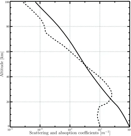
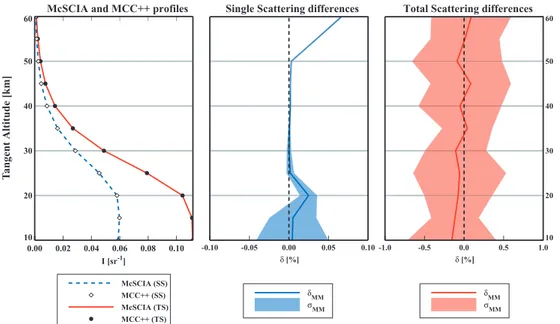
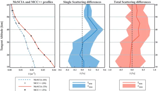
We compared with the first case of Loughman et al. (2004, Sect. 3.2, Fig. 4): a limb scan in an aerosol free atmosphere, forλ=_{345 nm and}_λ=_{325 nm. We use the}

15

MODTRAN (Berk et al., 1989) tropical atmospheric density and O3 profiles, with the cross section for Ozone and Rayleigh provided in theLoughman et al.(2004) (see also Table3). The vertical profiles ofkscaandkextare shown in Fig.8.

The atmosphere was discretized in 100 homogeneous layers equally spaced (1 km depth each), with the Earth radius set to 6377.640 km. For scattering the Rayleigh

20

phase function was used. Polarisation was neglected (scalar case).

The results of the intercomparison are shown in Figs. 9 and 10 for 345 nm and 325 nm, respectively, both for single scattering and total scattering, using the ET method.

The percentage diff_{erence between the two models is defined as}

25

(17)

ACPD

6, 1199–1248, 2006

F. Spada et al.

◭ ◮

Print Version

EGU The standard deviationσMMof the comparison is defined as

σMM=

q

σ_McSCIA2 +_σ2

MCC++. (19)

Generally the agreement between the two models is within twoσMM (grey region) and is better without (345 nm) than with (325 nm) O3absorption. The agreement is worse in the upper part of the scan than in the lower part for the case of 325 nm.

5

We think that these features have a common cause: we had to generate our own optical atmosphere for theLoughman et al.(2004) intercomparison case, so that some small diff_{erences exist between the two model set-ups. Another issue is that the}

ge-ometries used in McSCIA and in the intercomparison paper are not the same: we use angles at the top of the atmosphere instead of angles at the tangent altitude, and small

10

numerical errors can be introduced in the conversion. The diff_{erences between the two}

models are well under 0.2% for most cases and always smaller than 0.5%.

In conclusion we are confident that we correctly implemented absorption and the spherical geometry in our McSCIA model, and we have already a proof that the ET method gives good results.

15

5.2. Comparison between ET and SSA in 3-D

Here we want to investigate whether the ET approach gives equivalent results as the SSA approach in 3-D for a wide range of scenarios with diff_{erent absorption profiles.}

In particular we want to analyse extreme cases, in terms of optical thickness or vertical distribution. McSCIA simulations were performed with 1 million photons and the

atmo-20

spheric profiles were generated with Eq. (13) using the parameter values of Table4. As can be seen from Fig.11the ET and SSA results agree very well. The standard-ised diff_{erences between the two approaches are rarely larger than 0.5}_σ_{, and always}

smaller than one σ. More importantly, Fig. 11 shows a tendency towards a normal distribution of SD, like in Fig.7. However, in 3-D the computation time is much longer

25

(18)

ACPD

6, 1199–1248, 2006

F. Spada et al.

◭ ◮

Print Version

EGU Both approaches give the same results for diff_{erent scenarios with a variable amount}

of absorber, concentrated in one thin layer or spread over many layers. With McSCIA it is now possible to study several 3-D absorption scenarios with one simulation, thanks to the power of the Equivalence theorem.

6. Discussion

5

In this section we discuss diff_{erent implementations of the ET used in literature and the}

one used in McSCIA.

The aim of this paper is to show the validity of the ET approach in 3-D RT problems. This power of the ET approach has been recognised earlier. For instance,van de Hulst

(1980) states that RT can be defined in terms of inert parameters, i.e. variables that

10

determine the radiance field but remain constant in many equivalent situations. These inert parameters may be clouds, geometrical setting, phase function, etc.

Considering an atmosphere in which the haze provides scattering and absorption and a gas provides absorption, the ET can be summarised by (van de Hulst,1980, p. 576)

15

I(ω, τ, γ)=X

n

In(τ, γ=0)ωn

Z∞

0

pn(τ, γ =0, λ)e−γλdλ. (20)

whereω is the haze single scattering albedo, λ the optical path-length and γ is the ratio of the gas absorption to haze extinction. The equation tells that the radiance in an absorbing atmosphereI(ω, γ) can be calculated as a weighted sum over the number of scattering eventsnof the radianceI_n(γ=_{0) due to each scattering order calculated}

20

in a non-absorbing atmosphere. The weight contains the absorption, which is calcu-lated from the statistical part of the information in the form of the normalised probability distribution (pdf) of photon path-lengthsp_n(γ=₀_{, λ}_{), calculated for each scattering}

or-der. The important point here is that the pdf is calculated in an atmosphere without absorption and is subsequently used to calculate the absorption contribution.

(19)

ACPD

6, 1199–1248, 2006

F. Spada et al.

◭ ◮

Print Version

EGU In the work of Partain, Heidinger and Stephens (Partain et al., 2000; Stephens

and Heidinger,2000; Heidinger and Stephens, 2000,2002) the ET, as expressed by Eq. (20), has been presented and employed, extending the original formulation ofvan

de Hulst (1980). The use of geometrical instead of optical photon paths allowPartain

et al. (2000) to extend the ET to multiple homogeneous layers. The ET is actually

5

extended also in a way that takes into account ground albedo, the single scattering albedo and a vertical gas profile. The problem is solved by the introduction of a pdf that represents the statistics for gas, particle and ground absorption. Since storage of the complete pdf would make the model slower than performing SSA calculations, an approximate pdf is constructed. The authors recognised that such an approach

10

introduces a bias, i.e. an overestimate of the spectral absorption.

For the work of Cahalan et al. (1994) holds similar consideration as for the one of Partain.

Another approach was introduced byFeigelson (1984). The concept of equivalent trajectories is used to condense the information of all the individual photon trajectories

15

in an “average” trajectory. Basically this quantity represents the average number of times that a model layer has been crossed vertically by the “average” photon. In prin-ciple, such an average photon path calculated for a scattering-only atmosphere might be convolved with diff_{erent absorption profiles. However, it can be shown that this}

ap-proach is only valid in the weak absorption limit (i.e. exp(−τabs)=1−τabs). Apart from

20

the approximate nature of these approaches, they suff_{er also from the limitation that}

they cannot be used for 3-D varying absorption features.

None of these implementations of the ET compared the use of the ET and the tra-ditional SSA approach for a 3-D case. Thus, we extended the ideas outlined above by retaining all information of the scattering photons in a 3-D spherical atmosphere.

25

Although such an approach is not effi_{cient (storage of the scattering positions of}_≈106

(20)

ACPD

6, 1199–1248, 2006

F. Spada et al.

◭ ◮

Print Version

EGU selected scattering scenarios.

An issue that deserves improvement in McSCIA is the quality of the statistical infor-mation of photons. When atmospheric absorption is strongly dominant over scattering, simulations of a scattering-only atmosphere are not representative for the true situa-tion. For instance, in a scattering-only case many photons will travel to the surface

5

while in reality most of the photons would be subject to atmospheric absorption. A way to circumvent this problem is the use of a mixed SSA and ET approach. The conven-tional SSA method is used to simulate photon paths in an absorbing and scattering atmosphere (e.g. employing a standard absorption profile). Afterwards, 3-D absorp-tion perturbaabsorp-tions can be studied using the ET approach. Using this approach, the

10

statistical photon path information that is stored represents the actual situation more effi_ciently.

A strong point of our implementation is the possibility of using a 2-D varying ground albedo in a simple way. This is due to the fact that the ground albedo only appears in Eq. (10); it is very simple to relate its value to an albedo map.

15

The traditional way to use the ET is to employ the fact that scattering varies much less with wavelength than absorption, especially in spectral windows with sharp ab-sorption lines. This allow a fast calculation of abab-sorption lines under the assumption that scattering is constant. However, this is not the only way in which it can be used. After having demonstrated in this paper for the first time the validity of the ET in a

20

spherical 3-D environment, we are currently employing the ET to study the sensitivity of the TOA radiance for 3-D variations of absorption in the atmosphere (Spada and

Krol, 2005), by calculating 3-D weighting functions. This is relevant to e.g. satellite measurement of tropospheric pollution.

7. Summary and conclusions

25

(21)

ACPD

6, 1199–1248, 2006

F. Spada et al.

◭ ◮

Print Version

EGU study the radiances measured by limb-viewing instruments like SCIAMACHY. McSCIA

can use mixed Rayleigh and Henyey-Greenstein phase functions and can employ a 2-D varying Lambertian surface reflection. Refraction and polarisation are not included.

Results from the ray-tracing module compare well with published results for non-absorbing plane-parallel cases, for diff_{erent phase functions (Rayleigh and}

Henyey-5

Greenstein) and several nadir geometries and sun positions.

The spherical implementation of McSCIA was successfully validated against the state-of-the-art Monte Carlo model MCC++ ₍_Postylyakov_, ₂₀₀₄_{) and earlier results}

(Adams and Kattawar,1978;Kattawar and Adams,1978) simulating a homogeneous spherical shell atmosphere.

10

In McSCIA the absorption has been implemented using two diff_{erent methods. The}

traditional SSA methods which uses the scattering and absorption optical depth as vertical coordinate and employs the single scattering albedoωat the simulated scat-tering positions to take into account absorption of radiation. The ET approach which simulates photons in a scattering-only atmosphere and treats absorption afterwards by

15

convolving the individual photon paths with the associated absorption profile.

Using a simple 1-D model, we demonstrated that these two diff_{erent approaches}

give results that are identical in a statistical sense for a wide range of scenarios. A more in depth comparison between the two approaches is made using the spheri-cal implementation of McSCIA. Several scenario studies show that the ET and the SSA

20

approaches give equivalent results, even for extreme cases.

To our knowledge this is the first implementation of the Equivalence Theorem in a 3-D spherical RT model. This approach allows us to study the radiance field, simulated for a particular scattering geometry, as a function of 3-D atmospheric absorption fea-tures. For simulations with 106 photons, the relative error of McSCIA is normally well

25

(22)

ACPD

6, 1199–1248, 2006

F. Spada et al.

◭ ◮

Print Version

EGU (e.g. Walter et al., 20051). Moreover, McSCIA is one of the few models that allow the

study of 3-D varying absorption features in a spherical atmosphere. Currently, McSCIA is used to simulate 3-D absorption features for nadir and limb satellite measurements.

Appendix A: Mathematical background

A1. Radiative transfer laws and random numbers

5

Since RT processes are statistical in nature, most quantities in transfer theory can be easily interpreted as probabilities, or probability distributions.

In the Appendix the wavelength dependence has been omitted from the formulas to improve their readability.

The core is the fundamental principle of Monte Carlo simulations (Cashwell and

10

Everett, 1959; Marshak and Davis, 2005). For the continuous case, let p(x) be the normalised probability (PF), witha≤x<b:

Zb

a

dξp(ξ)=₁_.

Thenp(x)dx is the probability ofx lying betweenx and x+_d_x_{. The cumulative}

prob-ability functionP(x) (CPF) determinesx uniquely as a function of the random number

15

R:

R=_P₍_x₎=

Zx

a

dξp(ξ). (21)

Moreover, ifRis uniformly distributed on 0≤R<1, thenxfalls with frequencyp(x)dx in the interval (x, x+_d_x_).

1

(23)

ACPD

6, 1199–1248, 2006

F. Spada et al.

◭ ◮

Print Version

EGU Thus, the CPF is the quantity that relates a random number to physical processes.

We will show in the next sections some examples of this relation, guided by the pro-cesses that are implemented in McSCIA.

A2. Photon path length

The normalised probability PF(s) that a photon will travel through a medium from point 0

5

to pointsOikarinen et al.(see e.g.1999);Marshak and Davis(see e.g.2005), following Lambert-Beer’s law (Liou,1980), is

PF(s)= exp (−τs)

R∞

0 dτ

′

sexp −τs′

(0≤PF(s)≤1). (22)

The fundamental principle of Monte Carlo simulations must be applied to statistically derive the optical depth travelled, soR_τmust be equal to the normalised CPF

10

R_τ=

R∆τ

0 dτ

′

sexp −τ

′

s

R∞

0 dτ

′

sexp −τ

′

s

=1−exp (−∆τ) 0≤ Rτ <1. (23)

The statistical optical depth travelled before the next collision is then given by

∆_τ=−ln (1− R_τ) 0≤ R_τ <1. (24)

But, since 1−R_τ is still a random number between 0 and 1, Eq. (24) can be rewritten as

15

∆_τ=−ln (R′_τ) 0<R′_τ≤1 (25)

With a backward MC in limb view it is advantageous to bias this distribution, permitting the photons only to scatter in (0,∆_τ_max_{], so that the biased sampled photons do not}

leave the atmosphere at the first scattering event. In that case the sampling would be

∆_τ=−ln1− R_τ(1−exp(−∆_τ_max₎₎

0≤ R_τ <1. (26)

(24)

ACPD

6, 1199–1248, 2006

F. Spada et al.

◭ ◮

Print Version

EGU To account for this bias the weight of the photon has to be multiplied by 1−exp(−∆_τ_max_),

which simply states that a fraction of (1−exp(−∆_τ_max_{)) of all the photons leave the}

atmosphere after being emitted from the satellite.

A3. Scattering angles

When a photon is scattered by molecules (Rayleigh scattering) or aerosols and droplets

5

(Mie scattering) or is reflected from the ground, its direction changes. In order to find the new direction the scattering azimuth and zenith angles have to be simulated (see e.g.Oikarinen et al.,1999;Marshak and Davis,2005), in a statistical sense.

The rotation of the scattering anglesΘ_andΦ_{with respect to the atmospheric}

coor-dinate system are discussed in Sect.1.

10

A3.1. Scattering azimuth angle

The scattering azimuth angle, which determines the plane of the scattering event rela-tive to the reference direction, is uniformly distributed, that is

pΦ(Φ)=

1

2π (27)

so that applying Eq. (21)

15

Φ =₂_πRΦ 0≤ RΦ<1. (28)

A3.2. Scattering zenith angle

The scattering zenith angleΘ_{(relative to the incident direction) is determined from the}

scattering phase function. In the rest of the Appendix we will use, for simplicity, this notation

20

(25)

ACPD

6, 1199–1248, 2006

F. Spada et al.

◭ ◮

Print Version

EGU The rotation of the scattering angles anglesΘ_and Φ_{with respect to the atmospheric}

coordinate system are discussed in Sect.1

Rayleigh scattering

For Rayleigh scattering by air, the phase function for unpolarised light is (Liou,1980): P(µ)=3

4

1+_µ2 _µ∈[−1,1]. (29)

5

In this case Eq. (21) becomes R_µ= 1

2+ 1 8

3µ+_µ3 ₀≤ R_µ<1. (30)

This is a third order equation that can be solved exactly. Since the quadratic term is absent it is possible to use the “Formula Cardanica”. Equation (30) can be rewritten as:

10

µ3₊_pµ₊_q₌₀ ₍₃₁₎

p=_{3 and}_q=₄−8R_µ 0≤ R_µ<1 Since

∆ = q

2 4 +

p3

27 >0 0≤ Rµ<1

there is a real solution and two complex solutions. The real solution is:

15

µ=p3

a−q−p3

a+_q 3

r

1

2 (32)

q=₄−8R_µanda=

q

(26)

ACPD

6, 1199–1248, 2006

F. Spada et al.

◭ ◮

Print Version

EGU Henyey-Greenstein scattering

For scattering of photons in the UV-vis region on aerosols and droplets, Mie scatter-ing theory (see e.g. Lenoble, 1993) has to be used. A Mie scattering phase function is generally complicated, but a reasonable approximation is the Henyey-Greenstein function

5

P(µ)= 1−g

2

1+_g2₋₂_gµ3₂

(33)

whereg is the asymmetry factor. The relation between the scattering angle and the random number obtained using the fundamental principle of Monte Carlo simulations is

µ= 1

2g



1+g2−

1−g2 1−g+₂_gR_µ

!2

 0≤ R_µ<1 (34)

10

wheregis the asymmetry factor of the phase function defined as

g=_{< µ >}=

R+1

−1µp(µ)dµ

R+1

−1p(µ)dµ

. (35)

Mixed phase function

When the model has to take into account scattering from more than one type of parti-cles, a mixed phase function has to be used (Oikarinen et al.,1999). Supposekext(x)

15

represents the total volume extinction coeffi_{cient: absorption and scattering both by}

molecules and particles. In general, the profile will be a function of the 3-D positionx.

McSCIA needs to separate the extinction coeffi_{cient in scattering and absorption}

coeffi_cients:

kext₍_x₎₌_kabs₍_x₎₊_ksca₍_x₎ ₍₃₆₎

(27)

ACPD

6, 1199–1248, 2006

F. Spada et al.

◭ ◮

Print Version

EGU and then to separate the scattering coeffi_{cients in molecular and aerosol scattering}

ksca(x)=ksca mol(x)+ksca aer(x). (37)

The single scattering albedo is defined as usual ω(x)= k

sca (x)

kext₍_x₎. (38)

The ratio between molecular and total scattering is then represented by

5

fsca(x)= k

sca mol (x)

ksca₍_x₎ . (39)

For molecular scattering Eq. (29) is employed, and for aerosol scattering Eq. (33). At a scattering event first a random number is drawn to decide whether the scattering will be molecular or from aerosol:

R_sca≤fsca⇒use Eq. (32) R_sca> fsca⇒use Eq. (34)

10

When the exact scattering probability of scattering towards the sun has to be com-puted (see Eq.2) a mixed phase function expression is used

P(x, µ)=Pmol(µ)·fsca(x)+Paer(µ)·(1−fsca(x)) (40)

While the phase function for molecular scatteringPmol and aerosol scatteringPaer are taken to be independent of the positionx, the mixed phase function is a function of the

15

positionx.

A3.3. Lambertian surface reflection

When a photon reaches the surface and is reflected, the new direction is uniformly sampled. Thus Eq. (21) becomes

R_µ=

Zµ

0 dµ′_µ′

0≤ R_µ≤1 (41)

(28)

ACPD

6, 1199–1248, 2006

F. Spada et al.

◭ ◮

Print Version

EGU The relation between the scattering angle and the random number is then given by

µ=qR_µ 0≤ R_µ≤1. (42)

As for atmospheric scattering, the azimuth angle for surface reflection is calculated using Eq. (28). Since the direction of reflection it is defined only by the random number, it is easy to introduce a 2-D variability. This is only accounted for in the value of albedo

5

a(x_j) that is used to calculatewalb

i (see Eq.10). A3.4. Scattering angle to the sun

Equation (2) requires the angle between the photon direction and the solar rays. This angle can be calculated in spherical geometry as

µ_s_i(θ_idir, φdir_i , θsun_i , φsun_i )=_cos(_θdir

i ) cos(θ sun

i )+sin(θ dir i ) sin(θ

sun

i ) cos(φ dir i −φ

sun i ). (43)

10

The directional angles θdir_i and φdir_i are diff_{erent at each scattering event, while the}

solar anglesθsun and φsun are always the same, since a global reference system is used.

Alternatively, given positionsx

i−1,xi andx out

i (see Fig.1) the vector formula can be used

15

µsi(θ

dir i , φ

dir i , θ

sun i , φ

sun i )=

−−−−−→

x

i−1xi · −−−−→

x

ixout_i . (44)

A3.5. New photon direction

Calculation of the new direction of a photon after a scattering event, requires the old direction and scattering angles. The latter are calculated using Eqs. (28) and (32), (34) or (42). In the local reference system of the old direction the new direction is calculated

20

by two successive rotations ofΘ_andΦ_{, respectively, as illustrated in Fig.}₁_{. This new}

(29)

ACPD

6, 1199–1248, 2006

F. Spada et al.

◭ ◮

Print Version

EGU Acknowledgements. This research was supported by the GO EO-041 grant from the Space

Research Organisation of the Netherlands (SRON). The authors would like to thank H. Walter and J. Landgraf for many insightful discussions and the inter-comparison work. We are grateful also to R. Loughman for providing us the data necessary for the model validation.

References

5

Adams, C. N. and Kattawar, G. W.: Radiative transfer in spherical shell atmospheres 1. Rayleigh Scattering, Icarus, 35, 139–151 1978. 1204,1207,1208,1219,1231,1239,1240

Berk, A., Bernstein, L. S., and Robertson, D. C.: MODTRAN: A moderate resolution model for LOWTRAN-7, GL-TR-89-0122, Geophysics Laboratory, Hanscom AFB, MA 01732, 1989.

1214

10

Bovensmann, H., Burrows, J. P., Buchwitz, M., Frerick, J., Noel, S., Rozanov, V. V., Chance, K. V., and Goede, A. P. H.: SCIAMACHY: Mission Objectives and Measurement Modes, J. Atmos. Sci., 56, 127–150, 1999. 1201

Burrows, J. P., Weber, M., Buchwitz, M., Rozanov, V., Ladstatter-Weissenmayer, A., Richter, A., de Beek, R., Hoogen, R., Bramstedt, K., Eichmann, K., Eisinger, M., and Perner, D.: The

15

Global Ozone Monitoring Experiment (GOME): Mission concept and first scientific results, J. Atmos Sci., 56, 151–175, 1999. 1201

Cahalan, R., Ridgway, W., Wiscombe, W., Gollmer, S., and Harshvardhan: Independent pixel and Monte Carlo estimates of stratocumulus albedo, J. Atmos. Sci., 51, 3776–3790, 1994.

1202,1217

20

Cashwell, E. D. and Everett, C. J.: Monte Carlo Method for random walk problems, Pergamon Press, 1959. 1203,1220

Collins, D. G., Blattner, W. G., Wells, M. B., and Horak, H. G.: Backward Monte Carlo cal-culations of the polarization characteristics of the radiation emerging from spherical shell atmospheres, Appl. Opt., 11, 2684–2696, 1972. 1204

25

Davis, J., McKee, T., and Cox, S.: Application of the Monte Carlo method to problems in visibility using a local estimate: an investigation, Appl. Opt., 24, 3193–3205, 1985. 1204,1209

de Haan, J., Bosma, P., and Hovenier, J.: The adding method for multiple scattering calculations of polarized light, Astron. Astrophys., 183, 371–391, 1987. 1207

Feigelson, E. (Ed.): Radiation in a cloudy atmosphere, Kluwer, 1984. 1202,1209,1217

(30)

ACPD

6, 1199–1248, 2006

F. Spada et al.

◭ ◮

Print Version

EGU Flittner, D. E., Bhartia, P. K., and Herman, B. M.: O3 profiles retrieved from limb scatter

mea-surements: Theory, Geophys. Res. Lett., 27, 2601–2604, 2000. 1201

Heidinger, A. and Stephens, G. L.: Molecular Line Absorption in a Scattering Atmosphere. Part II: Application to remote Sensing in the O₂ A band, J. Atmos. Sci., 57, 1615–1634, 2000.

1217

5

Heidinger, A. and Stephens, G. L.: Molecular Line Absorption in a Scattering Atmosphere. Part III: Pathlength Characteristics and Effects of Spatially Heterogeneous Clouds, J. Atmos. Sci., 59, 1641–1654, 2002. 1217

Irvine, W.: The formation of absorption bands and the distribution of photon optical paths in a scattering atmosphere, Bulletin of the Astronomical Institutes of The Netherlands, 17, 266–

10

279, 1964. 1202,1208

Jacob, D. J.: Introduction to Atmospheric Chemistry, Princeton University Press, 1999. 1201

Kaiser, J.: Atmospheric Parameter Retrieval from UV-vis-NIR Limb Scattering Measurements, Logos Verlag, Berlin, Germany, 2002. 1201

Kaiser, J., von Savigny, C., Eichmann, K.-U., No ¨el, S., Bovensmann, H., Frerick, J., and

Bur-15

rows, J.: Satellite Pointing Retrieval from Atmospheric Limb Scattering of Solar UV-B Radia-tion, Canadian Journal of Physics, pp. 1041–1052, 2004. 1201

Kattawar, G. W. and Adams, C. N.: Radiative transfer in spherical shell atmospheres, II, asym-metric phase function, Icarus, pp. 436–449, 1978. 1207,1219,1231

Lenoble, J.: Radiative transfer in scattering and absorbing atmospheres: Standard

computa-20

tional procedures, A. Deepak Publishing, Hampton, Virginia, 1985. 1202,1203,1204

Lenoble, J.: Atmospheric Radiative Transfer, A. Deepak Publishing, Hampton, Virginia, 1993.

1224

Levelt, P. F., van den Oord, G. H. J., Dobber, M. R., Malkki, A., Visser, H., de Vries, J., Stammes, P., Lundell, J., and Saari, H.: The Ozone Monitoring Instrument, IEEE Transactions on

Geo-25

science and Remote Sensing, in press, 2005. 1201

Liou, K.-N.: An introduction to atmospheric radiation, Academic Press Inc., 1980. 1221,1223

Loughman, R., Griffioen, E., Oikarinen, L., Postylyakov, O., Rozanov, A., Flittner, D., and Rault, D.: Comparison of radiative transfer models for limb-viewing scattered sunlight measure-ments, J. Geophys. Res.-Atmos., 109, doi:10.1029/2003JD003854, 2004. 1214, 1215,

30

1233,1244