Hydroxyl (6±2) airglow emission intensity ratios for rotational
temperature determination
W. J. R. French1,2,G. B. Burns1,K. Finlayson1,P. A. Greet1,R. P. Lowe3,P. F. B. Williams1 1
Australian Antarctic Division, Kingston, Tasmania, Australia 7050
2Institute of Antarctic and Southern Ocean Studies, University of Tasmania, Hobart, Tasmania, Australia, 7000 3
Institute for Space and Terrestrial Science, University of Western Ontario, London, Canada N6A3K7
Received: 10 May 2000 / Accepted: 23 May 2000
Abstract. OH(6±2) Q1/P1 and R1/P1 airglow emission intensity ratios, for rotational states up to j¢= 4.5, are measured to be lower than implied by transition probabilities published by various authors including Mies, Langho et al. and Turnbull and Lowe. Exper-imentally determined relative values of j¢ transitions yield OH(6±2) rotational temperatures 2 K lower than Langho et al., 7 K lower than Mies and 13 K lower than Turnbull and Lowe.
Key words: Atmospheric composition and structure (airglow and aurora; pressure, density and temperature)
1 Introduction
Hydroxyl airglow emissions are used extensively for studies of the upper mesosphere (e.g. Oermann and Gerndt, 1990; Sivjee, 1992; Scheer, 1995). The emissions originate from a layer near 87 km with a mean thickness of 8 km (Baker and Stair, 1988).
Rotational temperatures are derived by comparing the intensities of two or more lines from dierent upper rotational states, as per Eq. (1) (Mies, 1974). Transition probabilities are used to apportion the percentage of the upper rotational states that decay via the transitions measured.
T hc=k Fb Fa=lnfIaAb 2j0b1g=fIbAa 2j0a1g
1
Fa,Fbare the energy levels of the initial rotational states (we use energy level values given by Coxon and Foster, 1982);Ia,Ibare the emission intensities of the OH lines
from dierent upper states; Aa, Ab are the transition probabilities; j0a, j0b are the upper state, total angular
momentum quantum numbers; and h, c and k are Planck's constant, the speed of light and Boltzmann's constant respectively.
Hydroxyl bands are designated by transitions from an upper state, v¢ (=vibration quantum number), to a lower state, v¢¢, as the OH(v¢±v¢¢) band. The Dv= 2 hydroxyl bands are the brightest. These occur in the near-infrared around 1.5 microns. As Dv increases the bands become less intense and appear at lower wave-lengths. Particular OH bands are popular depending on the upper wavelength limit of the detector. With a GaAs or cooled ccd detector the OH(6±2) band neark840 nm is often preferred (e.g. Myrabo and Harang, 1988; Viereck and Deehr, 1989; Scheer, 1995; Hecht et al., 1995; Hobbs et al., 1996; Greet et al., 1998); see Takahashi and Batista (1981) for a comparison of OH bands in the vicinity of (6±2).
The transition probabilities of Nelson et al., (1990), used by researchers for low Dv transitions (e.g. Lowe
et al., 1991; Sivjee and Waltershied, 1994; Mulligan
et al., 1995) do not cover the OH(6±2) band. Transition probabilities have been published that include the Dv= 4 band (e.g. Mies, 1974 = Mies; Turnbull and Lowe, 1989 = T&L; Langho et al., 1986 = LWR). The larger the vibrational transition, the larger is the temperature variance from the choice of transition probabilities (T&L). Greet et al. (1998) reported a 12 K variation in OH(6±2) temperatures depending on the choice of transition probabilities.
Intensity ratios of lines from the same upper state are constant, independent of temperature. We report mea-surements of line ratios from the four lowest quantum number rotational states of the OH(6±2) band for comparison with values inferred from Mies, LWR and T&L (see Table 1). Ratios of transition probabilities (the Aa/Ab values in Eq. 1) are experimentally derived from observations of the night sky. We also compare average temperatures derived from measurements of the four brightest OH(6±2) P1-branch lines, using spectra recorded at Davis, Antarctica (68.6°S, 78.0°E), and the
transitional probabilities of Mies, LWR, T&L and the experimentally determined Aa/Abratios.
2 Hydroxyl line nomenclature
This description of hydroxyl line nomenclature is condensed from Osterbrock and Martel (1992) and Osterbrocket al. (1996, 1997). Lines within an hydroxyl band principally result from rotational state transitions within either the ground or ®rst excited electronic state of the molecule. Rotational transitions within the excited state are about a third as intense as the equivalent ground state transition.
The hydroxyl electronic ground state is designated C2P
3/2 and has electronic total angular momentum
W= 1.5. The ®rst excited state, C2P1/2, has W= 0.5. The total rotational angular momentum of the molecule,
j, is the vector sum ofWand the angular momentum of nuclear rotation. The total angular momentum of the hydroxyl molecule can be any integral value above the electronic total angular momentum. Thus the ground state hasj= 1.5, 2.5, 3.5,. . ., and the ®rst excited state has j= 0.5, 1.5, 2.5, . . . . Alternatively, the rotational states can be designated by the total molecular angular momentum apart from spin. This is designatedk, and is an integral quantum number for describing the rotation states (used for example by Chamberlain, 1961). For the ground electronic state, k=j ), and for the ®rst
excited state,k= j+ .
Quantum selection rules limit rotational quantum number transitions to )1 (P-branch), 0 (Q-branch) and +1 (R-branch). Thus we can describe ground state rotational transitions as: OH(v¢±v¢¢) P(or Q, or R)1(k¢¢). Either the lower state rotational quantum numberk¢¢, or the upper state rotational quantum numberj¢, have been commonly used to describe the transitions. We choose to use k¢¢ as it is an integral value. The `1' subscript applies to a ground state transition. A `2' subscript implies a transition within the ®rst excited state.
Each rotational line is further split by L-doubling into components depending on the parity of the electronic wave functions to re¯ections in a plane through the internuclear axis. These transitions are distinguished by subscripts eandf, indicating the lower
state parity. Thus, OH(v¢±v¢¢) P,Q,R1,2e,f(k¢¢) distin-guishes theL-components. Typically theL-components are spectrally close, but the separation increases as the
k¢¢of the transition.
Weak transitions are possible between the two lowest electronic energy levels of the hydroxyl molecule. These are known as `satellite' lines, and have been observed and reported (Turnbull and Lowe, 1983; Osterbrock
et al., 1997; Greetet al., 1998). These are noted by aDk superscript preceding the Dj descriptor. Dk transitions ranging from)2 to +2 are possible and are designated
O,P,Q,R,S, in an expansion of theDjnomenclature. The electronic state transition is indicated by a double numeral sux in a `from ± to' manner. Thus PQ12(2) indicates an electronic state transition from the ground state to the ®rst excited state, with Dk=
)1 and
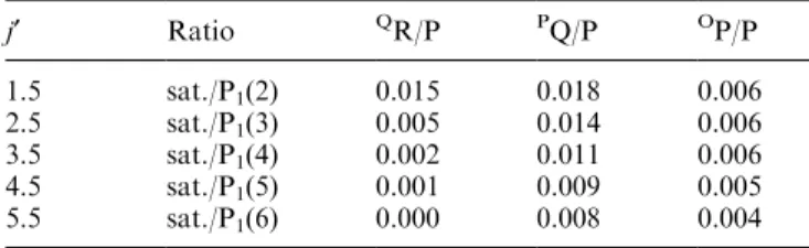
Dj= 0, with the lower state having a k quantum number of 2. Goldman (1982) gives transition proba-bilities for satellite lines relative to the Mies values for the main branch transitions. These are listed as ratios of the appropriate OH(6±2) P1-branch line intensities in Table 2.
Upper rotational states may thus emit via three possible transitions within their initial electronic state, or via three weak transitions between electronic states. It is the relative proportions emitted via these possible transitions that is allowed for by the Aa/Ab ratios of Eq. (1).
At some level of j¢, the rotation state populations become non-thermal (see e.g. Pendleton et al., 1993). States of high j¢ from one hydroxyl band may have wavelengths suciently dierent from the dominant band lines to extend into another band (see Osterbrock
et al., 1997; Greetet al., 1998).
3 Instrumentation and data
A Czerny-Turner scanning spectrophotometer (CZT) has been run for a number of years at Davis, Antarctica (68.6°S, 78.0°E). For the measurements reported here, the spectrophotometer had a six degree ®eld-of-view (fov) in the zenith. A cooled ()28°C) GaAs
photomul-tiplier tube was used for photon detection. A blocking ®lter (rejects k< 475 nm) was used, limiting observa-tions to the ®rst order. The instrument is described more completely by Greetet al. (1998).
The spectral response was determined by scanning a low brightness source (LBS) which uniformly illuminated
Table 1. Q1/P1 and R1/P1 ratios inferred from Mies, LWR and
T&L compared with measured values
j¢ Ratio T&L Mies LWR Experiment
1.5 Q1(1)/P1(2) 1.42 1.365 1.33 1.261 0.012
2.5 Q1(2)/P1(3) 0.49 0.46 0.44 0.389 0.006
3.5 Q1(3)/P1(4) 0.244 0.228 0.213 0.173 0.011
4.5 Q1(4)/P1(5) 0.145 0.132 0.123 0.094 0.004
5.5 Q1(5)/P1(6) 0.094 0.086 0.078
2.5 R1(1)/P1(3) 0.540 0.486 0.451 0.436 0.017
3.5 R1(2)/P1(4) 0.678 0.590 0.523 0.510 0.010
4.5 R1(3)/P1(5) 0.732 0.615 0.522 0.483 0.018
5.5 R1(4)/P1(6) 0.756 0.613 0.500
Table 2. Satellite line ratios with respect to the appropriate P-branch line, as inferred from Goldman (1982)
j¢ Ratio QR/P PQ/P OP/P
1.5 sat./P1(2) 0.015 0.018 0.006
2.5 sat./P1(3) 0.005 0.014 0.006
3.5 sat./P1(4) 0.002 0.011 0.006
4.5 sat./P1(5) 0.001 0.009 0.005
the CZT fov. The LBS was calibrated against a spectral standard by the Australian Measurement Laboratories. The CZT was used to spectrally scan the LBS a total of 121 times on ®ve separate occasions throughout the 1997 observation season (February±October). The LBS intensities at k828 nm and k851 nm, the largest separa-tion of lines compared, yielded a consistent ratio over the year to within 0.24%. An average instrument response is suitable for the entire 1997 data set.
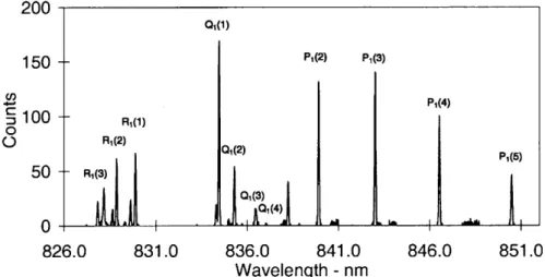
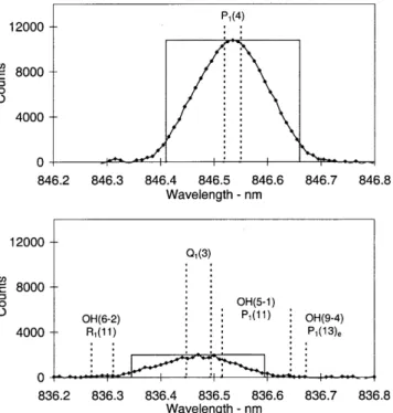
The operating mode for determining OH rotational temperatures during 1997 consisted of successively scanning narrow wavelength intervals incorporating the OH(6±2) P1(2), P1(4) and P1(5) emissions and appropriate background regions. Entrance and exit slit separations of 250 microns were used. Between day-of-year (DOY) 182±229, 1997, additional wavelength regions were successively incorporated, to measure the intensities needed to determine the low rotational quantum number (j¢ £4.5) line ratios. A step size of 0.01 nm and a dwell-time of 1 s were used. Between DOY 230±295, the slit separations were narrowed to 100 microns, reducing the width of the instrument function. This is near the limit to which reasonable parallelism of the entrance and exit slits can be maintained for this instrument. The step size was reduced to 0.005 nm and a dwell-time of 1 s maintained. The additional wavelength regions needed to determine individual line ratios were incorporated in separate campaigns over a number of nights, so that temperature measurements could be maintained. Figure 1 is a compilation of all spectral regions scanned.
Knowledge of the instrument function is needed to allow for contamination by lines not fully separated from adjacent features. A frequency stabilized laser was used to illuminate the entrance aperture and de®ne the instrument function at k632.82 nm. This de®ned the shape of the main passband and the location and magnitude of the ®rst and second Rowland `ghosts' (Longhurst, 1957). The measured instrument function was scaled to the OH(6±2) region, maintaining the shape of the main peak and the relative intensity of the ghosts. The displacement of the ghosts from the main peak was scaled in wavelength according to Dk¢/k¢= Dk/k.
The full-width-at-half-maximum (fwhm) of the instrument function at the OH(6±2) P1(4) wavelength (k846.5 nm) was determined by best ®tting the sum of two equal instrument functions, separated by the P1(4)
L-doublet separation (0.0305 nm) to an average mea-sured P1(4) pro®le. The P1(4) line was chosen for this determination in preference to the more intense P1(2) and P1(3) emissions because of contamination by Q1(5) and OH(5±1) P1(12)e respectively (Greet et al., 1998). The ghosts are assigned a shape similar to that deter-mined for the main peak.
At 100 micron slit separation, a slightly asymmetric, rounded instrument function of fwhm 0.071 nm is appropriate. The ®rst ghosts are approximately 0.33% of the main peak, and displaced by 0.354 nm. For the second ghosts, an approximate magnitude of 0.18% and displacement of 0.71 nm were estimated. At 250 micron slit separation, an instrument function with a fwhm of 0.155 nm was similarly determined.
During 1995 and 1996 spectra were collected as continuous scans from k837.5 nm to k851.5 nm. The step size was 0.005 nm, the dwell-time was 0.1 s and the slit widths were 250 microns. Five scans were combined to give a spectrum for temperature analysis. From this data set, 279 spectra obtained during optimal observing conditions and with no signi®cant auroral contamina-tion were chosen. These spectra are principally used to determine two satellite line ratios and to derive average temperatures from P1 line ratio pairs for a comparison of transition probabilities.
A broad classi®cation of sky conditions (clear, thin cirrus, patchy cloud, overcast, snow) was maintained through visual observation and reference to an all-sky video system. The `thin cirrus' classi®cation describes times when uniform thin high cirrus cloud, through which bright stars are visible, was apparent. In the cold Antarctic winters this is a common condition. Strato-spheric haze is also often present, however as it can only be seen in forward scattered sunlight e.g. at twilight, its presence is ignored.
Only spectra that are free of auroral contamination are used in the intensity ratio determinations. In selecting against auroral contamination, reference was
Fig. 1. A compilation of spectral regions scanned with 100 micron slit separations, normalized to 100 counts for the P1(4) peak
intensity. Major lines of interest arelabelled. Apparent but not labelled are: R1(4 + 5) at
made to wide-angle (60 degree fov), zenith-oriented photometer measurements of the auroral N21NG band atk428 nm.
Meteorological balloon ¯ights, by employees of the Australian Bureau of Meteorology, were conducted twice daily during 1997 at Davis. Measurements taken allow calculation of the equivalent column density of water vapour above the site (Sturman and Tapper, 1996). Reference is made to these data when water absorption of emissions may be signi®cant.
4 Determination of line ratios
The desired line intensities are determined after aligning and summing selected spectra. Unless speci®cally noted, spectra collected with 100 micron slit separations (0.071 nm fwhm instrument function) are used. The counts in a 0.125 nm region centred on the emission of interest are typically determined. The `count region' occasionally varies, as will be indicated, to allow for diculties with some emissions. A background level is determined for each emission of interest in the summed ®les. The fraction of an emission in the count region, and the contamination from nearby emissions, are determined using the instrument function. Allowance is made for L-doubling of the OH lines. It is assumed that individualL-components are of equal intensity. An estimate of the uncertainty in the derived ratios due to the uncertainty in the `®tted-to-P1(4)' instrument func-tion was obtained by comparison with the results obtained using an instrument function derived by scaling the laser wavelength pro®le up in wavelength to the OH(6±2) region. The largest dierence in any ratio was 0.2%, an amount insigni®cant compared with other uncertainties in the measurements.
The only absorber of consequence in the wavelength range covered is H2O. Using high-resolution telluric absorption spectra (HITRAN92; Rothman et al., 1992) and the technique described in Turnbull and Lowe (1983), the transmission of each L-component has been checked. Where absorption by water vapour may be of concern, it is noted in the speci®c ratio determinations.
The CZT is a scanning instrument. The P1(4) emissions in the 1995 and 1996 continuous scans (279 spectra) give an average intensity variation of )0.038% per minute, consistent with a tendency for decreasing hydroxyl intensity across the night at this site (Greetet al., 1998). The time dierence between measuring the line intensities used to determine desired ratios are listed in Table 3. The largest time dierence is 7.4 min [for determining Q1(4)/ P1(5)] and the shortest is 1.2 min [Q1(1)/P1(2)]. For each of the ratios determined, the P1(4) intensity is monitored, and the average P1(4) intensity over the summed spectra is calculated as a `percentage variation per minute'. These values are also listed in Table 3 along with the implied percentage error in the ratio being determined. The greatest uncertainty in the measured ratios, due to the time interval between measuring the individual intensi-ties, is)0.8% for the R1(3)/P1(5) ratio. No allowance is made for the minor variations possible due to the time interval between measuring the emissions.
The spectral response was determined from 121 separate scans of a calibrated LBS with an average curve suitable for our purposes, as previously indicated in Sect. 3. The standard deviation of the individual scans was used to estimate the uncertainty in the derived ratios due to the spectral response calibration. The uncertain-ties, no greater than 0.3% for any ratio, are also listed in Table 3 and are insigni®cant compared to other sources of error for all ratios.
A range of cloud conditions have been accepted for the ratios determined. A value determined from `clear sky' spectra is also presented for all ratios except the two satellite line ratios. No statistically signi®cant dierence is found between ratios determined under cloudy or clear conditions. In Table 3 are listed the number of spectra summed in determining each ratio and the sky conditions under which those spectra were acquired.
In determining some ratios, it was necessary to include spectra collected when the moon was above the horizon (see Table 3). Separate determination of the background for each emission allows for any spectral slope in moon-aected spectra. A solar spectrum was examined to ensure that Fraunhofer absorption did not aect the ratios determined.
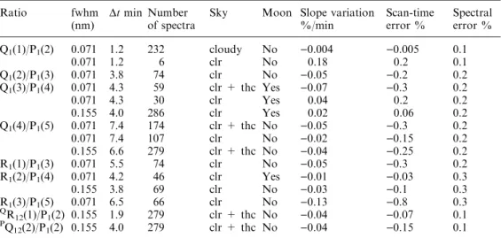
Table 3. Information on the data sets used to derive the in-dicated ratios. Included are the instrument function fwhm, the time taken to scan between the emissions, the number of spectra in the data set, the sky conditions (cloudy, clear = clr or thin cirrus = thc), whether the data set includes spectra collected when the moon was above the horizon, the average slope in the P1(4) intensity for
the data set, the error in the ratio implied by the average intensity slope and the spectral response error
Ratio fwhm
(nm)
Dtmin Number of spectra
Sky Moon Slope variation %/min
Scan-time error %
Spectral error %
Q1(1)/P1(2) 0.071 1.2 232 cloudy No )0.004 )0.005 0.1
0.071 1.2 6 clr No 0.18 0.2 0.1
Q1(2)/P1(3) 0.071 3.8 74 clr No )0.05 )0.2 0.2
Q1(3)/P1(4) 0.071 4.3 59 clr + thc Yes )0.07 )0.3 0.2
0.071 4.3 30 clr Yes 0.04 0.2 0.2
0.155 4.0 286 clr Yes 0.02 0.06 0.2
Q1(4)/P1(5) 0.071 7.4 174 clr + thc No )0.05 )0.3 0.2
0.071 7.4 107 clr No )0.02 )0.15 0.2
0.155 6.6 279 clr + thc No )0.04 )0.25 0.2
R1(1)/P1(3) 0.071 5.5 74 clr No )0.05 )0.3 0.2
R1(2)/P1(4) 0.071 4.2 46 clr Yes )0.01 )0.03 0.3
0.155 3.8 69 clr No )0.03 )0.1 0.3
R1(3)/P1(5) 0.071 6.5 66 clr No )0.13 )0.8 0.3 Q
R12(1)/P1(2) 0.155 1.9 279 clr + thc No )0.04 )0.07 0.1 P
An uncertainty is estimated for each ratio as the square-root of the sum of the squares of the relative errors of the individual line intensities. Emission inten-sity uncertainty includes allowance for counting statis-tics and uncertainties in estimates of the baseline, contamination by nearby emissions and any atmospher-ic absorption.
4.1 Q1(1)/P1(2) [j¢= 1.5]
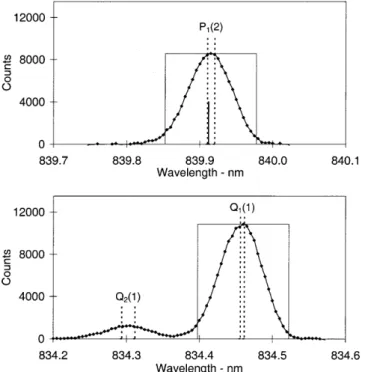
Two hundred and thirty-two spectra were summed to determine this ratio. All cloud conditions were accepted. Figure 2 shows the Q1(1) and P1(2) regions of the summed spectrum. Only 0.2% of the Q2(1) emission falls in the Q1(1) count region. Ninety-six percent of the Q1(5)fline and 1.3% of the Q1(5)e line (atk840.04 nm) lie in the P1(2) count region. For a temperature of 200 K, the estimates of the total intensity of the Q1(5) emission with respect to the P1(2) emission for Mies, LWR and T&L transition probabilities varies between 1.6±1.7%. The range for a temperature of 240 K is 2.7± 2.9%. A reasonable estimate of the Q1(5) intensity relative to the P1(2) intensity for winter temperatures above Davis is 2.2 0.8%. Taking Q1(5) contamina-tion of this level into account, the Q1(1)/P1(2) ratio is measured to be 1.261 0.012. This is the only ratio determined without any selection against cloud condi-tions. There were only six spectra collected under clear skies. These six spectra when combined yield a Q1(1)/ P1(2) ratio of 1.31 0.07. Variations in intensity in the 1.2 min between measuring the two emissions, deter-mined from variations in the P1(4) intensity, average out
to be insigni®cant ()0.005%, see Table 3). Dominant sources of uncertainty come from estimations of the P1(2) background and the Q1(5) contamination.
4.2R1(1)/P1(3) and Q1(2)/P1(3) [j¢= 2.5]
Seventy-four spectra were summed to determine the R1(1)/P1(3) and Q1(2)/P1(3) ratios. Figure 3 shows the R1(1), Q1(2) and P1(3) regions of the summed spectra. An estimated 61% of the unthermalized OH(5±1) P1(12)e line lies in the P1(3) count region. The OH(5±1) P1(12)f line is centred, 0.2 nm towards longer wavelengths from the peak of the P1(3) emission. From the summed spectrum, it is estimated that the OH(5±1) P1(12)fline is 1.0 0.6% of the P1(3) intensity. This is lower than, but within estimated uncertainties, the value determined by Greetet al. (1998).
Ninety-®ve percent of the OH(5±1) P2(10)f line and 55% of the P2(10)eline lie in the R1(1) count region. We
Fig. 2. The `count regions' for determination of the Q1(1)/P1(2) ratio
are indicated by rectangles centred on the relevant emissions. The wavelength of the Q1(5)fline atk839.91 nm, which contaminates the
P1(2) emission, ismarkedbut not labelled
Fig. 3. Spectral regions for evaluation of the Q1(2)/P1(3) and R1(1)/
P1(3) ratios. The locations of the contaminating lines, QP21(3)e at
k829.88 nm, OH(5±1) P2(10)fatk829.88 nm,QP21(3)fatk829.89 nm,
OH(5±1) P2(10)eatk829.95 nm and OH(5±1) P1(12)eatk843.07 nm,
assume that the intensities of these unthermalized lines are equal to the measured OH(5±1)P1(12)fintensity. An uncertainty amounting to 60% of the estimated con-tamination is ascribed. Ninety-®ve percent of the OH (6±2) satellite line QP21(3) also lies in the R1(1) count region. Goldman (1982) gives transition probabilities for the satellite lines consistent with Mies values for the major lines. For a temperature range of 200 K to 240 K, these transition probabilities yield QP21(3)/R1(1) ratios ranging from 0.95% to 1.25%. A ratio of 1.1% is used to estimate the QP21(3) contamination. We assign an uncertainty estimated as half the contamination value. The R1(1)/P1(3) ratio is measured to be 0.436 0.016. The principal uncertainty results from estimations of the contamination of the R1(1) measurement.
The Q1(2)/P1(3) ratio is measured to be 0.389 0.006. The main sources of uncertainty are in the determination of the baseline for the Q1(2) line and in estimating the OH(5±1) P1(12)econtamination of the P1(3) intensity.
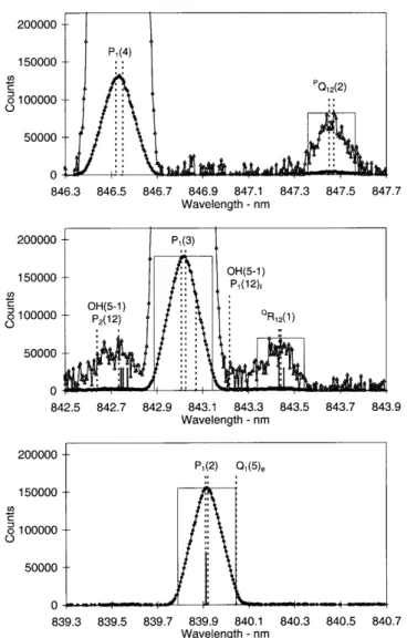
4.3 R1(2)/P1(4) [j¢= 3.5]
Forty-six spectra were summed for determination of the R1(2)/P1(4) ratio. Figure 4 shows the R1(2) and P1(4) regions of the summed spectrum. OH(9±4)P1(12)f is blended with R1(2), but OH(9±4)P1(12)eatk828.725 nm is not discernible (see Fig. 4), therefore no allowance is made for this contaminant. Water vapour is potentially an absorber of the R1(2) emission, but the atmosphere above Davis in winter is very dry. Meteorological balloon ¯ights at Davis station on the days these spectra were collected yield a water vapour column density of
1.8 1 mm cm)2. This implies only a 0.23% absorp-tion of the R1(2) emission. An R1(2)/P1(4) ratio of 0.514 0.013 is obtained from these spectra.
Sixty-nine spectra collected with 250 micron slit separations were also summed to obtain an independent estimation of this ratio. Count regions 0.25 nm wide centred on the respective emissions were selected. With this wider instrument function, it was necessary to allow for 6% of R2(3) under the R1(2) count region. Water vapour content was measured to be 3.5 1.5 mm cm)2, implying a 0.45% R
1(2) absorption. An R1(2)/ P1(4) ratio of 0.510 0.009 is measured. The larger number of suitable spectra, and the higher intensities obtained with the larger slit separations, yield a more accurate determination of the ratio. The principal source of uncertainty in both determinations comes from the background estimate for the R1(2) region.
4.4 Q1(3)/P1(4) [j¢= 3.5]
Fifty-nine spectra were summed to measure the Q1(3)/ P1(4) ratio. Seventy-two percent of the OH(5±1) P1(11)e emission lies in the Q1(3) count region. To obtain some estimate of the contribution of this feature, we assume it is of the same average relative magnitude as OH(5±1) P1(12)f which was measured in Sect. 4.2. Assuming an OH temperature of 220 K, the OH(5±1) P1(11)eemission amounts to 1.3% of the P1(4) intensity. The implied correction to the counts under the Q1(3) summing region is 5.5%. The Q1(3)/P1(4) ratio is measured to be 0.179 0.012. For the 30 `clear-sky' spectra in this data set, the Q1(3)/P1(4) ratio was 0.176 0.017. The principal sources of error come from estimation of the
Fig. 4. Summed spectral pro®les showing the R1(2) and P1(4) spectral
regions. OH(9±4) P1(12)fatk828.89 nm ismarkedwithout label
Fig. 5. Summed pro®les in the regions of Q1(3) and P1(4) obtained
OH(5±1) P1(11) contamination and the low intensity of the Q1(3) emission.
Two hundred and eighty-six ®les acquired with 250 micron slit widths were summed to obtain an indepen-dent estimation of the Q1(3)/P1(4) ratio. Count regions 0.25 nm wide centred on the respective emissions were used. Figure 5 shows the Q1(3) and P1(4) regions of the summed spectrum. Potential contaminants of the Q1(3) emission, measured with this larger instrument function, are OH(5±1) P1(11), OH(6±2) R1(11) and OH(9±4) P1(13)e. The OH(9±4) P1(13)e and OH(6±2) R1(11) contaminations are insigni®cant with respect to the uncertainty in the background level. The OH(5±1) P1(11)e line remains the principal contaminant, with 89% of its total intensity in the Q1(3) count region. Twenty-three percent of the OH(5±1) P1(11)f intensity also contaminates Q1(3). By assuming each is equivalent in average intensity to the measurement made of the OH(5±1) P1(12)f line, 7.7% of the counts in the Q1(3) count region are estimated to result from the OH(5±1) P1(11) emission. The Q1(3)/P1(4) ratio is thus 0.168 0.011. The principal uncertainty is in estima-tion of the OH(5±1) P1(11) contamination.
The similarity of the uncertainties associated with the Q1(3)/P1(4) determinations imply an average value, 0.173 0.011, is appropriate. We have not reduced the uncertainty, due to its strong dependence on the method used to estimate the OH(5±1) contamination.
4.5 R1(3)/P1(5) [j¢= 4.5]
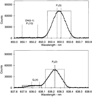
Sixty-six spectra were summed to determine the R1(3)/ P1(5) ratio. Figure 6 shows the R1(3) and P1(5) regions of the summed spectrum. The R1(3) region is very
crowded. An additional diculty is that R1(3) may be signi®cantly absorbed by atmospheric water vapour. The water column density over Davis when these spectra were acquired was measured to be 1.5 1 mm cm)2. For this level of atmospheric water vapour, the R1(3)f line at 828.164 nm is 0.45% absorbed and the R1(3)e component at 828.171 nm is 0.7% absorbed.
The R1(3) emission is signi®cantly contaminated on the low wavelength side by R2(4). Some allowance is made for this contamination by using an asymmetric R1(3) count region, from 0.0225 nm below the R1(3) centre wavelength to 0.0625 nm above. This reduces the R2(4) contamination of the R1(3) count region to 6.8% of the total R2(4) intensity. The R2(4) intensity is estimated by counting from the R2(4) centre wavelength, 0.0625 nm towards lower wavelengths. Ten percent of the total R1(6) intensity lies within the R1(3) count region. The R1(6) intensity is estimated using a count region from its centre wavelength, 0.0625 nm towards higher wavelengths. The R1(3)/P1(5) ratio is measured as 0.483 0.017. Uncertainties in the estimation of the R1(3) contaminants are the principal source of error.
4.6 Q1(4)/P1(5) [j¢= 4.5]
One hundred and seventy-four spectra were summed to determine a Q1(4)/P1(5) ratio of 0.107 0.009. The principal source of error is the low intensity of the Q1(4) emission.
The two hundred and seventy-nine spectra from 1995 and 1996 were used to independently determine the Q1(4)/P1(5) ratio. Figure 7 shows the Q1(4) and P1(5)
Fig. 6. Summed pro®les of the R1(3) and P1(5) spectral regions. The
R1(6)L-components are suciently close to be indistinguishable
Fig. 7. Summed pro®les of the Q1(4) and P1(5) regions obtained with
spectral regions of the summed ®le. The larger instru-ment function leads to an overlap of the P2(2) emission with the less intense Q1(4) emission. This is partially compensated by de®ning an asymmetric Q1(4) count region, from 0.1425 nm below the Q1(4) central wave-length to 0.0625 nm above (see Fig. 7). Less than 0.8% of the P2(2) emission contaminates this Q1(4) count region. A Q1(4)/P1(5) ratio of 0.094 0.004 is deter-mined. The uncertainty estimate is lower than for the 100 micron spectra due to increased Q1(4) photon counts. We use this more reliable estimate of the Q1(4)/ P1(5) ratio in further evaluations.
4.7 Satellite line ratios:PQ12(2)/P1(2)
andQR12(1)/P1(2) [j¢= 1.5]
The 279 spectra from 1995 and 1996 were used to estimate the ratios of two of the OH(6±2) satellite lines. Figure 8
shows the P1(2), QR12(1) [near P1(3)] and PQ12(2) [near P1(4)] regions of the summed spectrum. Also shown are the QR12(1) and
P
Q12(2) regions at 20 times magni®ca-tion, so as to better display the satellite lines.
The PQ12(2) intensity is estimated from a centred count region, 0.205 nm wide, and the P1(2) intensity is measured using a centred count region, 0.255 nm wide. The P1(2) count region is contaminated by 72.5% of the Q1(5) emission. The Q1(5) intensity is estimated to be 2.2 0.8% of the P1(2) intensity, as per Sect. 4.1. A P
Q12(2)/P1(2) ratio of 0.022 0.001 is determined. This is signi®cantly larger than the theoretical value of 0.018 determined from Goldman (1982). We have conserva-tively estimated the uncertainties possible from all known contaminants to the measured ratios, but if unknown contaminants exist their possible impact would be greatest on the lowest intensity features measured, such as the satellite lines.
TheQR12(1) emission has a number of contaminants. A count region 0.205 nm wide, centred on the QR12(1) emission was used. Contamination from the OH(5±1) P1(12) L-components is relatively minor, with 1.2% of the OH(5±1) P1(12) intensity contaminating theQR12(1) count region. As in Sect. 4.2, OH(5±1) P1(12)f was estimated as 1.0 0.6% of the total P1(3) intensity. More signi®cantly, the ®rst ghost of P1(3) contaminates the QR12(1) count region. This contamination amounts to 0.23% of the P1(3) intensity. The QR12(1) line is blended with QR12(4) (see Fig. 8). Goldman's (1982) transition probabilities give theQR12(4) intensity as 2.3% ofQR12(1) at 200 K and 3.1% at 240 K. A value of 2.7% was used to estimate theQR12(4) contamination. In total, 22% of the QR12(1) count region is estimated to come from contaminants. A QR12(1)/P1(2) ratio of 0.014 0.002 is determined. This is not signi®cantly dierent from the Goldman (1982) theoretical value of 0.015. Estimating the contamination of the QR12(1) count region is the greatest source of error, with the P1(3) ghost being the most signi®cant contaminant.
4.8 Comparison with published line ratios
Table 1 lists the line ratios calculated from the published transition probabilities of T&L, Mies and LWR, and the experimentally determined values. Experimental Q1/P1 ratios form a sequence signi®cantly lower than any of the theoretical values, but closest to LWR values. Measured R1/P1ratios are not signi®cantly dierent from the LWR values, but signi®cantly lower than those derived from T&L and Mies. The measured QR12(1)/P1(2) ratio of 0.014 0.002 is not signi®cantly dierent from the Goldman (1982) value, while thePQ12(2)/P1(2) value of 0.022 0.001 is signi®cantly higher. Table 2 lists the satellite line ratios calculated from Goldman (1982).
5 Comparison of temperature determinations
To derive a temperature from an OH(6±2) spectrum it is necessary to know the relative splitting of the upper
Fig. 8. Summed pro®les of the P1(2),QR12(1) and PQ12(2) regions
obtained with a 0.155 nm instrument function. The QR12(1) and P
Q12(2) regions are also shown at 20 times enhancement to enhance
the less intense emissions. The locations of the lines: Q1(5)f at k839.91 nm, QR12(2) at k842.74 nm and k842.75 nm, QR12(3)
at k842.77 nm, OH(5±1) P1(12)e at k843.07 nm, and QR 12(4) at
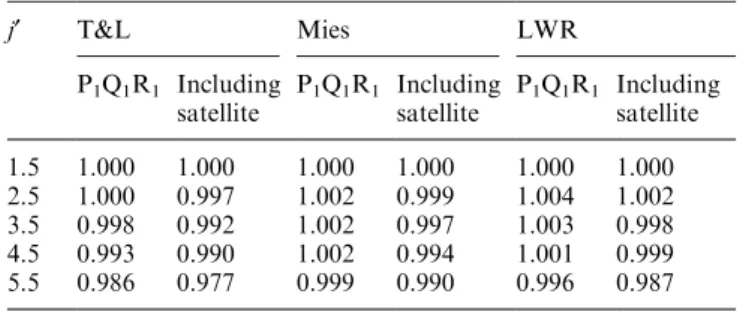
states of the emissions considered. The OH molecule is known to exhibit strong coupling of rotational and vibrational components (see e.g., Mies). If the relative proportions of the upper state that decay via the P, Q and R branches dier depending on theDvof the band, then the temperature independent ratios across all bands from the same vibrational upper state need to be measured before the relative splitting needed to deter-mine hydroxyl rotation temperatures can be derived. However, the strongest departure from branch balance between bands is exhibited by the weak Dv= 1 transitions. Table 4 lists the relativej¢-component sums of the of P1, Q1 and R1 branch transition probabilities across the (6±2) band for T&L, Mies and LWR. The variation between the upper states is less than 1%, up to
j¢= 4.5. A 1% error in the OH(6±2) P1(2)/P1(5) ratio corresponds to a 1 K error in the derived temperature. T&L, Mies and LWR do not list transition probabilities for the weak satellite lines, but if we incorporate Goldman (1982) values for the satellite lines as a proportion of the P1-branch transition (see also Table 4), the disparity up toj¢= 4.5 remains less than 1%. It is thus reasonable to estimate the relative proportions of the upper state that decay via the various branches within the (6±2) band as a percentage of the transitions within that band.
It has not been possible to measure all the ratios required up to the desired level of j¢= 4.5, but those missing are mainly low-intensity satellite lines. The measurements that have been made can be extrapolated to estimate the ratios required, or the best available theoretical estimates can be used to supplement the experimental measurements. The QR12(1)/P1(2) ratio measured was equal to the Goldman (1982) theoretical value. No measured estimates of OP12/P1 ratios are available. Thus, for the required QR12/P1 and OP12/P1 ratios, the values of Goldman (1982) are used. For the P
Q12/P1ratios, the measured value is used for P
Q12(2)/ P1(2) [j¢= 1.5] and the other required values are scaled proportionally. An uncertainty of half the estimated intensity is used for satellite lines for which no direct measurement is available. In this manner we can derive the fraction of the upper state that decays via each transition, up to j¢= 4.5. To make an allowance for Q1(5) which is blended with the P1(2) emission, values forj¢= 5.5 are required. A R1(4)/P1(6) ratio of 0.48 and
a Q1(5)/P1(6) ratio of 0.06 are selected as consistent with the trends of the measured ratios. Table 5 lists the fraction of the upper state that decays via each transi-tion up toj¢= 5.5.
Average temperatures for each of the six possible intensity ratios from the four brightest P1-branch lines from the 279 1995 and 1996 spectra are presented in Table 6 for Mies, LWR and T&L transition probabilities, and for the experimentally determined probabilities. The uncertainties listed in Table 6 are the standard deviations divided by the square-root of the number of spectra. A `weighted sum' temperature is derived as a sum of the average temperatures determined from the P1(2)/P1(4), P1(2)/P1(5) and P1(4)/P1(5) ratios, weighted inversely as the square of the standard deviation for those ratios. Temperatures derived using the P1(3) intensity are not included in the weighted sum because of contamination by non-thermalized OH(5±1) P1(12). As noted by other authors (for example: Turnbull and Lowe, 1989; Greetet al., 1998), the average temperature derived using the T&L transition probabilities is 6 K higher than for Mies values and 11 K higher than for LWR values. The temperature inferred from the experimentally deter-mined `same-upper-state' line ratios is within the mea-surement uncertainty of the LWR value.
The average temperatures derived from ratios using the P1(3) intensity with Mies and T&L transition probabilities show evidence of the OH(5±1) P1(12) contamination. Greet et al. (1998) used this evidence, and T&L transition probabilities, to estimate the average magnitude of the OH(5±1) P1(12) contamination. The average temperatures derived using the LWR transition probabilities show reduced evidence of this contamina-tion, indicating that the magnitude of the contamination estimated in this manner is dependent on the choice of
Table 4. The relativej¢-component sums of the of P1, Q1and R1
branch transition probabilities across the (6±2) band for T&L, Mies and LWR. Also shown are the relative sums determined by including the satellite lines from Goldman (1982). Each ratio is set to 1 forj¢= 1.5
j¢ T&L Mies LWR
P1Q1R1 Including
satellite
P1Q1R1 Including
satellite
P1Q1R1 Including
satellite
1.5 1.000 1.000 1.000 1.000 1.000 1.000 2.5 1.000 0.997 1.002 0.999 1.004 1.002 3.5 0.998 0.992 1.002 0.997 1.003 0.998 4.5 0.993 0.990 1.002 0.994 1.001 0.999 5.5 0.986 0.977 0.999 0.990 0.996 0.987
Table 5. Experimentally determined fractions of the upper state that decays via each branch within the OH(6±2) band
j¢ P1-branch Q1-branch R1-branch
1.5 0.434 0.002 0.548 0.003
2.5 0.539 0.008 0.209 0.003 0.235 0.009 3.5 0.587 0.007 0.101 0.006 0.299 0.004 4.5 0.627 0.008 0.059 0.002 0.303 0.011
5.5 0.643 0.039 0.308
Table 6. Average temperatures derived from the 279 1995 and 1996 spectra using the T&L, Mies and LWR transition probabil-ities, compared with the values obtained using the experimentally determined relative intensity ratios. Ratios that include P1(3) do
not contribute to the `weighted sum'. (see text)
Ratio T&L Mies LWR Experiment
P1(2)/P1(3) 222.0 1.5 211.7 1.3 204.3 1.3 200.7 1.2
P1(2)/P1(4) 213.5 0.8 206.2 0.7 200.3 0.7 198.8 0.7
P1(2)/P1(5) 212.7 0.7 206.4 0.7 201.6 0.6 199.4 0.6
P1(3)/P1(4) 209.3 0.9 203.7 0.8 198.8 0.8 198.8 0.8
P1(3)/P1(5) 210.5 0.7 205.3 0.7 201.3 0.6 199.4 0.6
P1(4)/P1(5) 212.5 1.0 207.5 1.0 204.1 0.9 200.8 0.9
transition probabilities. The temperatures inferred from the P1(2)/P1(3) ratio are most sensitive to contamination of P1(3). That there is no evidence for OH(5±1) P1(12) contamination in the averages of the experimentally determined temperatures may result from underestima-tion of the Q1(5) contamination of P1(2). Thej¢= 5.5 experimental estimates are extrapolations, and the intra-band balance of this state (see Table 4) is least certain. If this is the reason for the lack of a signature of the OH(5± 1) P1(12) contamination, then the implied error in the experimentally derived weighted temperature average is of the order of )1 K. The principal conclusion that the
OH(6±2) rotational temperatures are signi®cantly lower than are determined using Mies and T&L transition probabilities remains valid.
6 Conclusions
Q1/P1ratios for OH(6±2) band lines withj¢up to 4.5 are measured to be signi®cantly lower than implied by the three published sets of transition probabilities consi-dered.
R1/P1ratios for OH(6±2) band lines withj¢up to 4.5 are measured to be signi®cantly lower than implied by T&L and Mies transition probabilities, and lower than LWR values but on the borderline of signi®cance.
Two satellite line ratios are measured. The measured Q
R12(1)/P1(2) ratio is consistent with, while PQ12(2)/ P1(2) is measured to be 20% larger than, Goldman (1982) theoretical values.
OH(6±2) band rotational temperatures inferred from a set of experimentally determined fractions of j¢-state transitions are 2 K lower than temperatures derived using LWR transition probabilities, 7 K lower than temperatures derived using Mies values and 13 K lower than values derived using T&L values.
It is important to note that no implication can be drawn from our experimental measurements with re-spect to the absolute values of the transition probabil-ities. The variation in the absolute values between the three published sets of OH(6±2) transition probabilities is far greater than the variation in their temperature-invariant line ratios. T&L transition probabilities are approximately 350%, 395% and 460% greater than LWR ratios for the low j¢, P1-, Q1- and R1-branch transition probabilities respectively. The Mies transition probabilities are similarly approximately 130%, 140% and 150% greater than the LWR values. For compar-ison, the Q1/P1and R1/P1Mies, T&L and LWR ratios compared dier by between 3% and 18%. Our conclu-sion that LWR OH(6±2) transition probabilities yield rotational temperatures most consistent with experi-mental measurements provides no direct evidence that the absolute values of LWR transitional probabilities are experimentally preferred.
Acknowledgements. This project has been supported by the Ant-arctic Science Advisory Committee and the Australian AntAnt-arctic Division. The Australian Bureau of Meteorology provided mete-orological balloon data from Davis, Antarctica. A.R. Klekociuk provided valuable assistance with discussions and access to
programs for deriving H2O column densities. Davis station
Australian National Antarctic Research Expeditioners from 1995±1997 have supported the collection of these data.
Topical Editor F. Vial thanks M.J. Taylor and F.J. Mulligan for their help in evaluating this paper.
References
Baker,D. J.,and A. T. Stair,Rocket measurements of the altitude distributions of the hydroxyl airglow,Phys. Scr.,37,611±622, 1988.
Chamberlain,J. W.,Physics of the aurora and the airglow, Academic, New York, 1961.
Coxon,J. A.,and S. C. Foster,Rotational analysis of hydroxyl vibration-rotation emission bands: molecular constants for OH X2P, 6£v£10,Can. J. Phys.,60,41±48, 1982.
Goldman,A.,Line parameters for the atmospheric band system of OH,Appl. Opt.,21,2100±2102, 1982.
Greet,P. A.,W. J. R. French,G. B. Burns,P. F. B. Williams, R. P. Lowe,and K. Finlayson,OH(6±2) spectra and rotational temperature measurements at Davis, Antarctica,Ann. Geophys-icae,16,77±89, 1998.
Hecht,J. H.,S. K. Ramsay Howat,R. L. Waltershied,and J. R. Isler, Observations of variations in airglow emissions during ALOHA-93,Geophys. Res. Lett.,22(20), 2817±2820, 1995. Hobbs,B. G.,I. M. Reid,and P. A. Greet,Mesospheric rotational
temperatures determined from the OH(6±2) emission above Adelaide, Australia,J. Atmos. Terr. Phys.,58(12), 1337±1344, 1996.
Langho,S. R.,H.-J. Werner,and P. Rosmus,Theoretical transition probabilities for the OH Meinel system, J. Mol. Spectr.,118,507±529, 1986.
Longhurst,R. S.,Geometrical and physical optics, Longmans, London, 1957.
Lowe,R. P.,K. L. Gilbert,and D. N. Turnbull,High-latitude summer observations of the hydroxyl airglow, Planet. Space Sci.,39(9), 1263±1270, 1991.
Mies,F. H.,Calculated vibrational transition probabilities of OH(X2P),J. Mol. Spectrosc.,
53,150±180, 1974.
Mulligan,F. J.,D. F. Horgan,J. G. Galligan,and E. M. Grin, Mesopause temperatures and integrated band brightnesses calculated from airglow OH emissions recorded at Maynooth (53.2°N, 6.4°W) during 1993, J. Atmos. Terr. Phys., 57(13), 1623±1637, 1995.
Myrabo,H. K.,and O. E. Harang,Temperatures and tides in the high-latitude mesopause region as observed in the OH night airglow emissions,J. Atmos. Terr. Phys.,50(8), 739±748, 1988. Nelson,Jr.,D. D.,A. Schiman,and D. J. Nesbitt,H + O3
Fourier-transform infrared emission and laser absorption stud-ies of OH(X2P) radical: an experimental dipole moment function and state-to-state Einstein A coecients, J. Chem. Phys.,93(10), 7003±7019, 1990.
Oermann,D.,and R. Gerndt,Upper-mesosphere temperatures from OH* emissions, Adv. Space Res.,10(12), 217±221, 1990. Osterbrock,D. E.,and A. R. Martel,Sky spectra at a light-polluted
site and the use of atomic and OH sky emission lines for wavelength calibration,Publ. Astron. Soc. Pac.,104,76±82, 1992. Osterbrock,D. E.,J. P. Fulbright,and T. A. Bida,Night-sky high-resolution spectral atlas of OH and O2emission lines for Echelle
spectrograph wavelength calibration II,Publ. Astron. Soc. Pac., 109,614±627, 1997.
Osterbrock,D. E.,J. P. Fulbright,A. R. Martel,M. J. Keane,S. C. Trader,and G. Basri,Night-sky high-resolution spectral atlas of OH and O2emission lines for Echelle spectrograph wavelength
calibration,Publ. Astron. Soc. Pac.,108,277±308, 1996. Pendleton,W. R.,P. J. Espy,and M. R. Hammond,Evidence for
non-local-thermodynamic-equilibrium rotation in the OH nightglow,J. Geophys. Res.,98,11 567±11 579, 1993.
A. Perrin,A. Glodman,S. Massie,L. Brown,and R. Toth,The HITRAN molecular data base: Editions of 1991 and 1992, J. Quant. Spectrosc. Radiat. Transfer,48,469±507, 1992. Scheer,J.,What can be learned from rotational temperatures
derived from ground-based airglow observations about the aeronomy of the southern hemisphere,Adv. Space Res.,16(5), 61±69, 1995.
Sivjee,G. G.,Airglow hydroxyl emissions,Planet. Space Sci.,40, 235±242, 1992.
Sivjee,G. G.,and R. L. Waltershied,Six-hourly zonally symmetric tidal oscillations of the winter mesopause over the South Pole station,Planet. Space Sci.,42,447±453, 1994.
Sturman,A. P.,and N. J. Tapper,The weather and climate of Australia and New Zealand, Oxford University Press, Mel-bourne, 1996.
Takahashi,H.,and P. P. Batista,Simultaneous measurements of OH(9,4), (8,3), (7,2), (6,2) and (5,1) bands in the airglow, J. Geophys. Res.,86(A7), 5632±5642, 1981.
Turnbull,D. N.,and R. P. Lowe,Vibrational population distribu-tion in the hydroxyl night airglow,Can. J. Phys.,61,244±250, 1983.
Turnbull,D. N.,and R. P. Lowe,New hydroxyl transition probabilities and their importance in airglow studies,Planet. Space Sci.,37,723±738, 1989.
Viereck,R. A.,and C. S. Deehr,On the interaction between gravity waves and the OH Meinel (6±2) and the O2Atmospheric (0±1)