www.scielo.br/rbg
COMPARISON OF THE OH (8-3) AND (6-2) BAND ROTATIONAL TEMPERATURE
OF THE MESOSPHERIC AIRGLOW EMISSIONS
Cristiano Max Wrasse
1, Hisao Takahashi
2and Delano Gobbi
3Recebido em 8 outubro, 2004 / Aceito em 10 novembro, 2004 Received October 8, 2004 / Accepted November 10, 2004
ABSTRACT.The airglow OH (8-3) and (6-2) band rotational temperatures were measured and compared using two scanning photometer at Cachoeira Paulista (23˚S, 45˚W) in 1999. The rotational temperature were obtained from the ratio between the P1(5) and P1(3) in the case of the (8-3) band and P1(4) and P1(2) lines for the (6-2) band. Three different Einstein coefficients, of Mies (1974), Langhoff et al., (1986) and Turnbull & Lowe (1989) were used and compared between them. It was shown that both the temperature did agree well with in an error range when the Langhoff et al.’s coefficients were used.
Keywords: Mesosphere, hydroxyl, rotational temperature, Einstein coefficients.
RESUMO.A temperatura rotacional das bandas da OH(8-3) e OH(6-2) foram medidas e comparadas utilizando dois fot ˆometros de filtro inclin´avel, em Cachoeira Paulista (23˚S, 45˚O) no ano de 1999. A temperatura rotacional foi determinada atrav´es da raz˜ao entre as linhas rotacionais P1(5) and P1(3) para o caso da banda (8-3) e entre as linhas rotacionais P1(4) e P1(2) para a banda (6-2). Os coeficientes de Einstein publicados por Mies (1974), Langhoff et al., (1986) e Turnbull & Lowe (1989) foram utilizados para o c´alculo da temperatura e seus resultados foram comparados. Os resultados encontrados mostram que as temperaturas das bandas OH(8-3) e OH(6-2) s˜ao similares, dentro da margem de erro, quando os coeficientes de Einstein de Langhoff et al. foram utilizados.
Palavras-chave: Mesosfera, hidroxila, temperatura rotacional, coeficientes de Einstein.
Instituto Nacional de Pesquisas Espaciais (INPE), Caixa Postal: 515; CEP: 12245-970 – S˜ao Jos´e dos Campos, SP, Brasil. Phone: (12) 3945-7167; Fax: (12) 3945-6740. 1E-mail: [email protected]
INTRODUCTION
The airglow Hydroxyl emissions have been extensively used for studying atmospheric temperature variation in the mesopause re-gion since Meinel (1950) published its usefulness (Greet et al., 1998, Bittner et al., 2000). The OH emission originates from a layer near 87 km of altitude with a thickness of around 8 km (Baker & Stair, 1988). The temperature in the mesopause region is highly variable, between 150 and 250 K, depending on the geo-graphic location, local time, season and dynamical processes, such as tides and gravity waves (Waltersheid et al., 1987). The OH rotational temperature is one of useful parameters to monitor such variable atmospheric temperature in the mesopause region.
There are several reasons for using the OH rotational line spectrum to measure the mesopause temperature. The collision frequency of OH with the neutral atmosphere in the vicinity of 90 km of altitude should be in an order to 104s−1and the life
time of the excited OH is around 3 to 10 msec. (Mies, 1974). It indicates that the excited OH molecules in the rotational energy levels are in a thermal equilibrium with the atmospheric ambient gas (Sivjee & Hamwey, 1987, Takahashi et al., 1998). The other reason to use the OH spectra is that the rotational line spectra is open structure, separating 1 to 2 nm between the lines, which makes easy to measure individual lines by even low resolution (∼1 nm) spectrometer. Further, the line intensities of a band are only a function of the rotational temperature. Therefore using two lines from a single band one can estimate the rotational tempera-ture by the following equation (Mies, 1974):
Tn,m=
Eν′(Jm′)−Eν′(Jn′)
klnIn
Im
A(J′
m,ν′→J
′′
m+1,ν′′)
A(J′
n,ν′→Jn′′+1,ν′′)
2J′
m+1
2J′
n+1
(1)
Where Tn,m is the rotational temperature estimated from two
line intensities, In and Im, from rotational levels J′ n, J
′ m in
the upper vibrational levelν′, to J′′ n+1, J
′′
m+1in the lower
vi-brational level ν′′. Eν(J) is the energy of the level(J, ν). A(Jn′, ν′ → J′′
n+1, ν
′′)is the Einstein coefficient, for the
tran-sition fromJn′, ν′toJm′′, ν′′.
The OH rotational temperatures have been measured using several different bands, for example, (9-4), (8-3), (6-2), (4-2) and (3-1) bands with a combination of different Einstein coefficients, Mies (1974) (hereafter Mies); Langhoff et al. (1986) (hereafter LWR); Turnbull & Lowe (1989) (hereafter TL); and Nelson et al. (1990). This different combination of measurement has been gi-ving significant ambiguity in determination of the rotational tem-perature as pointed out by French et al. (2000). Table 1 shows
re-cent OH temperature measurement carried out by different groups in the world.
It seems that the Einstein coefficients for the OH ground state and lower vibrational levels are consistent between the different calculations (Nelson et al., 1990). For the upper vibrational le-vels, however, the coefficients show a certain discrepancy between them. The relative intensities calculated by the TL coefficients are the highest and those calculated by LWR are the lowest (Golden, 1997). Calculation of the Einstein coefficients depends on preci-sion of the electric dipole moment function and the wave function used. Error range of the two functions will increase in the higher vibrational and rotational levels. These are the factors that intro-duce discrepancy between the rotational temperatures.
Table 1– OH temperature measurement by different groups, different bands and different Einstein coefficients.
Tabela 1–Temperatura da OH medida por diferentes grupos de pesquisas, utilizando diferentes bandas da OH e diferentes Coeficientes de Einstein.
Author Band Coefficient French et al. (2000) OH (6-2) LWR Scheer & Reisin (2000) OH (6-2) Mies Takahashi et al. (1999) OH (6-2) Mies Taylor et al. (1999) OH (6-2) Mies and LWR Shiokawa et al. (1999) OH (6-2) TL Greet et al. (1998) OH (6-2) TL Williams (1996) OH (8-3) Mies Bittner et al. (2000) OH (3-1) Mies Espy & Huppi (1997) OH (3-1), OH (4-2) Mies Mulligan et al. (1995) OH (3-1), OH (4-2) TL and Nelson
et al. (1990)
We designed and constructed a portable OH(8-3) rotational temperature photometer and installed it at Brazilian Antarctic sta-tion at King George Is. (62˚S, 50˚W) in 2000. Prior to that the photometer has been operated at Cachoeira Paulista airglow ob-servatory (23˚S, 45˚W) for 4 months in 1999 in order to compare with the OH (6-2) rotational temperature observed at the same lo-cation. In the present work, therefore, we calculate the OH ro-tational temperature using the OH (8-3) and (6-2) band spectra, and compare between them using different Einstein coefficients published by Mies, TL and LWR.
INSTRUMENTATION AND DATA ACQUISITION
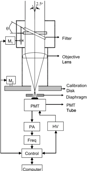
systems. Figure 1 shows the schematic diagram of the photo-meter illustrating main part of the instrument. The optical system is composed by a near infrared interference filter with a diameter of 45 mm, 1.0 nm wavelength resolution, an objective lens, an internal calibration disk, a field stop diaphragm and a S20 PMT tube. The field of view is2.5×8◦, which corresponds to an area
of about4×12km at the OH emission layer (around 87 km of
altitude). The electronics controls PMT high voltage (HV), pre-amplifier (PA) and discriminator (Freq), as well as the step motor M1 for filter tilting and M2 for calibration disk rotating. All of the systems are controlled by a computer.
2.5o Calibration Disk Diaphragm Filter Objective Lens θ PMT Tube M2 M1 Computer PMT Control Freq PA HV 2.5o Calibration Disk Diaphragm Filter Objective Lens θ PMT Tube M2 M1 Computer PMT Control Freq PA HV
Figure 1– Schematic diagram of the portable photometer illustrating the main parts of the equipment.
Figura 1–Esquema ´optico e diagrama de blocos do fotˆometro port´atil.
The photometer absolute sensitivity, counts/Rayleigh, was ca-librated using a MgO screen illuminated by a laboratory sub-standard light source (Eppley ES 8315 calibration lamp). A
tri-tium gas activated phosphor light source mounted in the disc was used for the day to day calibration of the sensitivity. The overall photometer sensitivity was around 3 counts/Rayleigh. This is low compared to the other ordinary airglow photometers, and requests longer time integration in order to get a good signal to noise ratio. One wavelength scan to get the P1(5) and P1(3) line spectra takes
20 seconds. After 10 continuous scanning an integrated spectrum is obtained, then the temperature was calculated. Estimated ins-trumental errors originating from filter transmission functions and uncertainty in the absolute sensitivity for the intensity and tempe-rature are±6% and±3 K, respectively, and the random error are
±5% and±6 K.
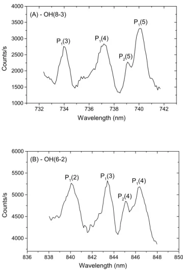
Fig. 2(A) shows an example of the OH(8,3) spectrum mea-sured by the photometer, where the OH(8-3) P branch lines can be identified. The P1(3), P1(4) and P1(5)lines can be traced by
tilting the filter scanning the wavelength from 732 to 742 nm. The intensity ratio between P1(5) and P1(3) was used to calculate the
rotational temperature, and this ratio has a larger temperature de-pendence compared to the other combination.
On the other hand, the OH (6-2) band P1(2), P1(3) and P1(4)
lines were measured by MULTI-2, a tilting filter photometer, de-signed to scan the wavelength from 838 to 848 nm with the wave-length resolution of 1.0 nm (Melo et al., 1993). Fig. 2(B) shows a measured spectra of the OH(6-2) P branch. A large optical di-ameter (60 mm) and a high sensitivity PMT tube (GaAs) made it possible to achieve a reasonably high throughput, around 20 counts/Rayleigh, which is much higher than that of the portable photometer. A rectangular field of view of2×7◦covers the OH
emission layer with an area of3×11km over the zenith at∼87 km
of altitude. The intensity ratio between P1(4) and P1(2) was used
to calculate the rotational temperature, which has a large tempe-rature dependence compared to the other combinations such as P1(3) and P1(2). The P1(3) line was not used because of that
there are P1(12) and P2(12) lines of the OH (5-1) band near of it at
843 nm, and it is difficult to estimate the contamination of these li-nes. Only a single scan was necessary to determine a temperature. Estimated instrumental errors originating from filter transmission functions and uncertainty in the absolute sensitivity for the inten-sity and temperature are±10% and±2 K, respectively, and the random error ranges are±2% and±3.5 K for each measurement (Takahashi, 1999).
The observations of the OH (6-2) band emission has been carried out at Cachoeira Paulista (23◦S,45◦W), during 1998 and
emis-732 734 736 738 740 742 1000
1500 2000 2500 3000 3500 4000
(A) - OH(8-3)
P1(5)
P1(4)
P2(5) P1(3)
C
o
u
n
ts
/s
Wavelength (nm)
836 838 840 842 844 846 848 850
4000 4500 5000 5500 6000
(B) - OH(6-2)
P1(4) P1(3)
P2(4) P1(2)
C
o
u
n
ts/
s
Wavelength (nm)
Figure 2– (A) Typical spectra of the OH (8-3) observed by the portable photometer and (B) the spectra of the OH (6-2) observed by the MULTI-2 photometer, where are showing the main rotational lines in the P branch used to calculate the temperature of the (8-3) and (6-2) OH bands.
Figura 2–Em (A) ´e apresentado o espectro do OH (8-3) observado pelo fotˆometro port´atil e em (B) ´e apresentado o es-pectro do OH (6-2) observado pelo fotˆometro MULTI-2, mostrando as principais linhas de emiss˜ao utilizadas para o c´alculo da temperatura do OH(8-3) e OH(6-2).
sions were carried out at the same place from August to November 1999. A total of 19 nights of data was obtained and used for the comparison. The three Einstein coefficients, Mies, TL and LWR, were used to compare the rotational temperature between them.
RESULTS AND DISCUSSION
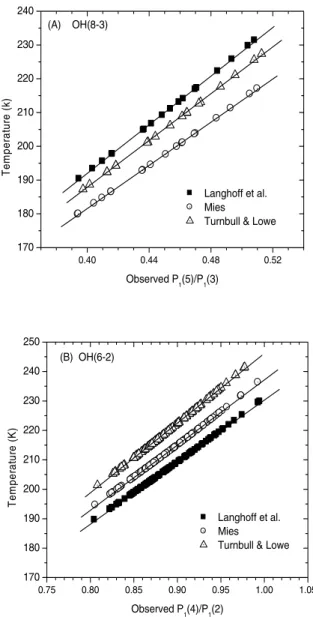
The nocturnal mean values of the OH (8-3) rotational temperature (hereafter T83)observed by the portable photometer from August
to November 1999 are shown in Fig. 3(A). Temperatures calcu-lated by using Mies, TL and LWR are plotted as a function of the observed intensity ratio between P1(5) and P1(3). The straight
li-nes in the figure represent a linear trend of the temperatures. The
figure shows that the temperatures calculated by the Mies coeffi-cients are the lowest (circles) and the temperatures of the LWR co-efficients are the highest (squares). The difference between them is not constant, but increasing with temperature, i.e., from 10 K around 180 K to 15 K around 230 K.
The nocturnal mean rotational temperatures of the OH (6-2) band (hereafter T62)observed by MULTI-2 photometer between
In Table 2 overall averaged temperatures and the standard de-viations of T83 and T62, for the data from August to November
1999 are summarized. For T83calculated using the LWR
coeffi-cient is 12 K higher than Mies and 3 K higher than TL. T62using
the TL coefficients is 13 K higher than LWR and 8 K higher than Mies.
Table 2– Overall averaged rotational temperatures of the OH (8-3), T83, and OH (6-2), T62, and the standard deviation (SD), in Kelvin. Data: 19 nights from August to November 1999.
Tabela 2–Temperatura rotacional m´edia de todas as noites da OH(8-3), T83, e OH (6-2), T62, e o desvio padr˜ao (SD) em Kelvin. Dados coletados em 19 noites entre agosto e setembro de 1999.
T83(K) T62(K)
Mean SD Mean SD Mies 196.8 11.5 214.1 8.3 TL 205.6 12.2 221.9 8.3 LWR 209.1 12.8 209.3 9.2
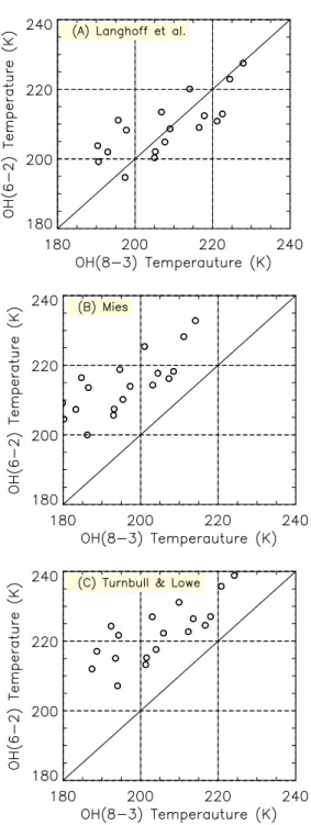
In order to compare the temperatures of the OH (8-3) and (6-2) emissions, the nocturnal mean values are plotted for the diffe-rent transition probability groups, Mies, LWR, and TL, in Figure 4. As expected from the Figure 3, there is a good agreement in the mean temperatures between T83and T62for the LWR coefficients
(209 K). For the Mies and TL coefficients, however, large differen-ces in the temperatures, around 16 K, can be seen. The plots are rather scattered around the linear relation line in the figure. This might be due to the difference of random error range of the two dif-ferent photometers. In Table 3, the difference in the temperature between T83and T62are summarized.
Table 3– Temperature difference between OH (8-3) and OH (6-2) band.
Tabela 3–Diferenc¸a entre as temperaturas das bandas da OH (8-3) e OH (6-2).
Einstein Coefficients T62-T83(K)
LWR +0.2
Mies +17.2
TL +16.2
The difference of temperature between the three transition probabilities, Mies, LWR and TL, shown in Fig. 3 are not obser-vational result, but it came from the difference of the transition probabilities used as can be seen in the Eq.(1). It should be noted that the difference, more than 12 K, is large and we should keep in mind it when the OH rotational temperature is used to monitor the atmospheric temperature in a vicinity of the mesopause around 85 to 90 km.
170 180 190 200 210 220 230 240
0.40 0.44 0.48 0.52
Langhoff et al. Mies
Turnbull & Lowe
Observed P1(5)/P1(3)
Te m p er a tur e ( k )
(A) OH(8-3)
170 180 190 200 210 220 230 240 250
0.75 0.80 0.85 0.90 0.95 1.00 1.05
Langhoff et al. Mies Turnbull & Lowe
Observed P1(4)/P1(2)
Te m p er at ur e ( K )
(B) OH(6-2)
Figure 3– Nocturnal mean rotational temperatures as a function of the obser-ved intensity ratio for the different Einstein coefficients, Mies (1974), Langhoff et al. (1986) and Turnbull & Lowe (1989), of the OH (8-3) band (A), and (B) of the OH (6-2) band, observed at Cachoeira Paulista (23˚S, 45˚W).
Figura 3–(A) M´edia noturna da temperatura rotacional da OH (8-3) em func¸˜ao das raz˜oes de intensidades observadas para os diferentes coeficientes de Eins-tein de Mies(1974), Langhoff et al. (1986) e Turnbull & Lowe (1989). Em (B) o mesmo para a banda da OH (6-2). Os dados foram obtidos em Cachoeira Paulista (23˚S, 45˚O).
The difference of temperature between the OH (8-3) and (6-2) emissions from one transition probability to the others showed in the Fig. 4 is significant. A good agreement between the two tem-peratures can be seen in the case of LWR. The small difference of 0.2 K should not be called much attention if we look into the scattered points in the Fig. 4 and the instrumental error ranges of the two photometers, which is around±5 K. The temperature
tran-sition probabilities, however, are much larger than expected from the instrumental error range.
Figure 4– Comparison of the observed OH (8-3) and (6-2) temperatures using Langhoff et al. (1986) transition probabilities (A), Mies (1974) (B), and Turnbull & Lowe (1989) (C).
Figura 4–Comparac¸˜ao da temperatura rotacional das bandas da OH (8-3) e (6-2) usando os coeficientes de Einstein de Langhoff et al em (A), Mies (1974) em (B) e Turnbull & Lowe (1989) em (C).
There is another possibility to give a different temperature in the two emissions. If the emission heights are different and the
atmospheric temperature has a gradient with height, the weigh-ted mean temperatures of the two bands could be different. Past rocket measurements (Lopez-Moreno et al., 1987) report that the difference between the emissions from the upper vibrational levels
(ν=7)and the lower ones(ν=2)could be as much as 5 km.
On the other hand, McDade (1991), concluded that the height dif-ference from the upper vibrational level(ν = 9)to the lower
one(ν = 1)should not be more than one or two kilometers.
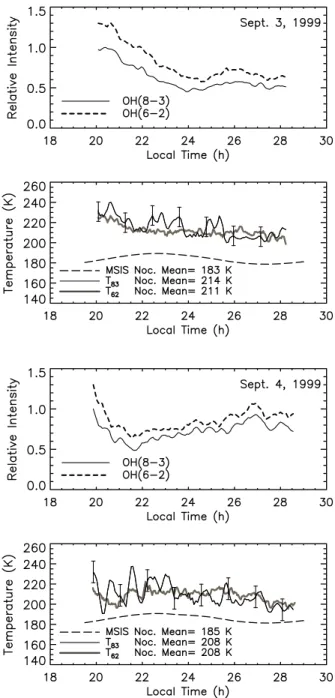
Whether the two emission layers are different with height or not, we can check it by looking into phase difference of their nocturnal intensity variations. In case of the gravity waves and tidal oscil-lations, their phase propagations are normally from the upper to lower heights. If the OH (8-3) emission profile is higher than OH (6-2), the former leads the latter. In order to check it, the intensity variations of the 19 nights were investigated using time lagged cross correlation analysis. No significant time lag (larger than 10 minutes) between the two emissions was found. In Fig. 5 typical nocturnal variations of the intensity and the rotational temperature on the night of September 3 and 4 are shown. Well correlated va-riation patterns of the OH (8-3) and (6-2) intensities can be seen. For the temperature calculation the LWR coefficients were used for both the emissions. The large variance of T83is due to the low
sig-nal to noise ratio of the OH (8-3) band observation on this night, resulting in a larger random error. From these results we conclude that the difference in the temperature between OH (8-3) and (6-2) should not be caused by their height difference and possible temperature gradient, neither the instrumental errors. The diffe-rence should be originated from the transition probabilities used. French et al. (2000) reported that the OH (6-2) band temperature calculated by LWR had a better agreement with their experimental values than those calculated by Mies and TL. Our present results and their discussion, therefore, lead a conclusion of that the LWR transition probabilities should provide a temperature of the OH emission layer better than the others, at least for the case of OH (8-3) and (6-2) band observations. For comparison of the present OH rotational temperatures with model atmosphere, the tempera-tures of MSIS-90 (Hedin, 1991) are also plotted in the figure. The MSIS-90 temperature shows similar nocturnal variation, but with much lower values,∼20 K, compared to the OH rotational tem-perature, which should be further investigated.
CONCLUSION
diffe-Figure 5– Nocturnal variations of the OH (8-3) and (6-2) band intensities and rotational temperatures observed at Cachoeira Paulista on September 3rd and 4th, 1999. Transition probabilities used are given by Langhoff et al. (1986). The rotational temperatures are also compared with the MSIS-90 model that showed the lowest values of temperature. The local time is expressed in decimal time and varies from 18 to 30 hours (18 to 06 hours of the next day).
rent Einstein coefficients show that the LWR coefficients provide the highest values and the Mies provides the lowest values. For the OH (6-2) band the higher temperatures values are from the TL coefficients and the lowers due the LWR coefficients. A good agre-ement in the rotational temperatures between the OH (8-3) and (6-2) bands was obtained when the LWR coefficients were used. The portable OH temperature photometer is in operation at Brazilian Antarctic Station (62˚S, 58˚W) since 200. The temperature data are available under request to authors.
ACKNOWLEDGEMENTS
The present work has been supported by CAPES and CNPq, under contract PROANTAR project No. 55.0355/02-2.
REFERENCES
BAKER DJ & STAIR JAT. 1988. Rocket Measurements of the Altitude Dis-tributions of the Hydroxyl Airglow. Physica Scripta, 37(4): 611–622.
BITTNER M, OFFERMANN D & GRAEF H. 2000. Mesopause temperature variability above a midlatitude station in Europe. Journal of Geophysical Research, 105(D2): 2045–2058.
ESPY PP & HUPPI R. 1997. The intertropical convergence zone as a source of short-period mesospheric gravity waves near the equator. Jour-nal of Atmospheric and Solar-Terrestrial Physics, 59(13): 1665–1671.
FRENCH WJR, BURNS GB, FINLAYSON K, GREET PA, LOWE RP & WIL-LIAMS PFB. 2000. Hydroxyl (6-2) airglow emission intensity ratios for rotational temperature determination, Annales Geophysicae, 18(10): 1293–1303.
GOLDEN SA. 1997. Kinetic parameters for OH nightglow consistent with recent laboratory measurements. Journal of Geophysical Research, 102(A9): 19969–19976.
GREET PA, FRENCH WJR, BURNS GB, WILLIAMS PFB, LOWE RP & FIN-LAYSON K. 1998. OH (6-2) spectra and rotational temperature measure-ments at Davis, Antarctica. Annales Geophysicae, 16(1): 77–89.
HEDIN AE. 1991. Extension of the MSIS Thermosphere Model into the Middle and Lower Atmosphere, Journal of Geophysical Research, 96(A2): 1159–1172.
LANGHOFF SR, WERNER HJ & ROSMUS P. 1986. Theorical transitions-probabilities for the OH Meinel system. Journal of Molecular Spectros-copy, 188(2): 507–529.
LOPEZ-MORENO JJ, RODRIGO R, MORENO F, LOPEZ-PUERTAS M & MOLINA A. 1987. Altitude distribution of vibrationally excited states of atmospheric hydroxyl at levels v = 2 to v = 7, Planet. Space Sci., 35: 1029–1038.
MCDADE IC. 1991. The altitude dependence of the OH (X2PI) vibrational distribution in the Nightglow: Some model expectations., Planet. Space Sci., 39: 1049–1057.
MEINEL AB. 1950. OH Emission Bands in the Spectrum of the Night Sky. I, Transactions-American Geophysical Union, 31 (21).
MIES FH. 1974. Calculated vibrational transitions probabilities of OH (X2). Journal of Molecular Spectroscopy, 53: 150–188.
MELO SML, GOBBI D, TAKAHASHI H, TEIXEIRA NR, LOBO R. 1993. O fotˆometro MULTI-2 Experiˆencia de calibrac¸˜ao – 1992. S˜ao Jos´e dos Campos: INPE, (INPE-5526, NCT/310).
MULLIGAN FJ, HORGAN DF, GALLIGAN JG & GRIFFIN EM. 1995. Meso-pause temperatures and integrated band brightness calculated from air-glow OH emission recorded at Maynooth (53,2˚N, 6.4˚W) during 1993. Journal of Atmospheric and Solar-Terrestrial Physics, 57(13): 1623– 1637.
NELSON DD, SCHIFFMAN A, NESBIT DJ, ORLANDO JJ & BURKHOL-DER JB. 1990. H + O3Fourier-transform infrared emission and laser
ab-sorption studies of OH (X2)radical: An experimental dipole moment
function and state-to-state Einstein A coefficients. Journal of Chemical Physics, 93(10): 7003–7019.
SCHEER J & REISIN SR. 2000. Unsual low airglow intensities in the Southern Hemisphere midlatitude mesopaude region. Earth Planets and Space, 52(4): 261–266.
SHIOKAWA K, KATOH Y, SATOH M, EJIRI MK, OGAWA T, NAKAMURA T, TSUDA T & WIENS RH. 1999. Development of Optical Mesosphere Ther-mosphere Imagers (OMTI). Earth Planets and Space, 51(7-8): 887–896.
SIVJEE GG & HAMWEY RM. 1987. Temperature and chemistry of the polar mesopause OH. Journal of Geophysical Research, 92(A5): 4663– 4672.
TAKAHASHI H, BATISTA PP, BURITI RA, GOBBI D, NAKAMURA T, TSUDA T & FUKAO S. 1998. Simultaneous measurements of airglow OH emis-sion and meteor wind by a scanning photometer and the MU radar. Jour-nal of Atmospheric and Solar-Terrestrial Physics, 60(17): 1649–1668.
TAKAHASHI H, BATISTA PP, BURITI RA, GOBBI D, NAKAMURA T, TSUDA T & FUKAO S. 1999. Response of the airglow OH emission, temperature and mesopause wind to the atmospheric wave propagation over Shinga-raki, Japan. Earth Planets and Space, 51(7-8): 863–875.
TAYLOR MJ, PENDLETON WR-JR., GARDNER CS & STATES RJ. 1999. Comparison of diurnal tidal oscillations in mesospheric OH rotational temperature and Na lidar temperature measurements at mid-latitudes for fall/spring conditions. Earth Planets and Space, 51(7-8): 877–885. TURNBULL DN & LOWE RP. 1989. New hydroxyl transitions probabili-ties and this importance in airglow studies. Planetary and Space Science, 37(6): 723–738.
WALTERSCHEID RL, SCHUBERT G & STRAUS JM. 1987. A dynamical-chemical model of the wave-driven fluctuations in the OH nightglow. Journal of Geophysical Research, 92(A2): 1241–1254.
NOTES ABOUT THE AUTHORS
Cristiano Max Wrasse.Physicist at Universidade Federal de Santa Maria (UFSM), 1997. Msc (Space Geophysics) at Instituto Nacional de Pesquisas Espaciais (INPE), 2000. PhD (Space Geophysics) at Instituto Nacional de Pesquisas Espaciais (INPE), 2004. Areas of interest: Equatorial and Polar Optical Aeronomy.
Hisao Takahashi.Bsc (Physics) at Niigata University – Japan, 1968. Msc (Upper Atmosphere) at Niigata University – Japan, 1970. PhD. (Space Science) at Instituto de Pesquisas Espaciais – INPE, 1980. Areas of interest: Optical Aeronomy.