Infrastructure privatization in a neoclassical economy: macroeconomic impact and welfare computation

..

ｾＣＢｆｕｎｄａￇￃｏ＠

ｾ＠

GETULIO VARGAS

EPGE

Escola de Pós-Graduação em

Economia

"Il\TI'BAS'l'BUC'l!UBE

PBIV A'l'IZA'l'IOl\T 1l\T A

l\TEOCLASSICAI· ECOl\TOlVIY:

ｄｬａｃｂｏｅｃｏｬ｜ｔｏｾｃｉｍｐａｃＧｬＧ＠

AlID WBLJ' ARE COMPUTA'l'IOl\T"

PEDRO CA V ALCANTI FERREIRA

(EPGE/FGV)

LOCAL

Fundação Getulio Vargas

Praia de Botafogo, 190 - 10° andar - Auditório

DATA

23/01/97 (5

a

_feira)

,

HORARIO

16:00h

Infrastructure Privatization in a Neoclassical Economy:

Macroeconomic Impact and Welfare Computation*

Pedro C. Ferreira

Escola de Pós-Graduação em Economia Fundação Getulio VargaslRJ

Abstract

In this paper a competi tive general equilibrium model is used to investigate the welfare and long run allocation impacts of privatization. There are two types of capital in this model economy, one private and the other initially public ("infrastructure"), and a positive extemality due to the latter is assumed. A benevolent governrnent can improve upon decentralized allocation intemalizing the extemality, but it introduces distortions in the economy through the finance of its investments. It

is shown that even making the best case for public action - maximization of individuais' welfare, no operation inefficiency and free supply to society of infrastructure services - privatization is welfare improving for a large set of economies. Hence, arguments against privatization based solely on under-investment are incorrect, as this maybe the optimal action when the financing of public investment are considered. When operation inefficiency is introduced in the public sector, gains from privatization are much higher and positive for most reasonable combinations of parameters.

•

1 -_Introduction

Infrastructure and privatization of public utilities have been, in the past years,

subject of a large literature and moved to the center of the policy debate in countries

around the world, both developed and developing. On the one hand, the productive impact

of infrastructure has been investigated lately by an increasing number of studies, starting

with Aschauer's pioneer paper(l989). These studies use different econometric techniques and data samples to estimate the output and productivity elasticity to public capital.

Overall, although the magnitudes found vary considerably, the estimates (e.g. Aschauer

(1989), Ferreira(l993), Duffy-Deno and Eberts(l991), Easterly and Rebelo(1993)) tend to

confirm the hypothesis that infrastructure capital positively affects productivity and

output, despite some important exceptions (e.g. Holtz-Eakin(l992) and Hulten and

Swchartz(l992)} On the other hand, the perception of poor performance of public owned infrastructure utilities, among other reasons, led to a flurry of privatization and

concessions in a large and increasing number of countries. For instance, from 1988 to

1992, revenue from infrastructure privatization in developing countries summed 19.8

billions of dollars (World Bank(l994)) and since then its pace has accelerated remarkably.

In this paper we use a competitive general equilibrium model, basically a variation

of the neoc1assical growth model, to investigate the welfare and Iong run allocation impacts ofprivatization. There are two types of capital in this modeI economy, one private

and the other public ("infrastructure"), and a positive externality due to the latter is

assumed. A benevolent govemment can improve upon decentralized allocation

internalizing the externality. However, it is assumed that lump sum taxation is not an option and that the govemment uses distortionary taxes to finance investment. This Iast

feature introduces a trade-off in the public provision of infrastructure, as distortionary

taxes may offset the productive effect - internaI and externaI - of public capital. The net

effect of privatization and other quantitative properties of this theoretical economy depend to a large extend on the relative strength of the two effects .

This model economy was solved using simulation techniques on the lines of

Kidland and Prescott( 1982), although the model is non stochastic. Model' s parameters and functional forms were calibrated following the tradition of real business cyc1e models of

•

values of the internaI and externaI effect of infrastructure capital, given the large and

conflicting nurnber of estimates in the literature. We chose, therefore, to use more than one

value for the externaI effect parameter and compare the results.

After solving the mode!, it was used to measure the welfare effect of privatization

under alternative sets of parameters and to compare long run allocations. One of the main

results is that, even making the best case for public action - maximization of individuaIs'

welfare, no operation inefficiency and free supply to society of infrastructure services

-privatization maybe welfare improving. Hence, argurnents against -privatization based

solely on under-investment are mistaken, as this maybe the optimal action when the

financing of public investment are considered. When operation inefficiency is introduced,

gains from privatization are much higher and positive for most reasonable combinations of

parameters.

On apure theoretical ground, Devarajan, Xie and Zou(1995) investigate alternative

systems of infrastructure services provision using distortionary taxes and part of our model

borrow heavily from theirs. However, they work in an endogenous growth environment

while we work with the traditional neoclassical growth mode!. This framework was chosen

because, in order to obtain sustainable growth, it is necessary to assume empirically

implausible values for the infrastructure coefficient in the production function. In other

worlds: if we consider the usual capital share of 0.36, the coefficient of infrastructure in a

Cobb-Douglas production function would have to be 0.64 for the model to display

sustainable growth. But the values estimated in the literature range from zero to 0.4, and

even this last value (Aschauer's (1989) estimate) was discredited on methodological

grounds (Gramlich(1994».

This paper is organized as follows. Section two presents the model with public

provision of infrastructure, section three presents the model without govemment ( i.e.,

after privatization), section 4 brief1y discusses calibration and section 5 discusses

methodology and presents the main results of the simulations. Finally, in section 6 some

•

2 -Model I: Public Infrastructure

In this economy a single final good is produced by finns from labor, H, and two types of capital, K and G. There is a positive extemality generated by the average of

capital G, G, so that the technology of a representative finn is given by:

(1)

In this first model, labor and K, private capital, are owned by individuaIs who rent

them to finns. The second type of capital, infrastructure (G), is owned by the governrnent,

who finance its investments by tax collection and supply G for free to finns. Hence, the

problem of a representative finn is to pick at each period the leveIs of private capital and

labor that maximize its profit, taking G, G and prices as given:

From the solution of this simple problem we obtain the expressions for the rental rate ofprivate capital, r, and wages, w:

(2)

(3)

A representative agent is endowed with one unit of time which he divides between

labor and leisure (l). His utility at each period is defined over sequences of consumption and leisure, and it is assumed that preferences are logarithm in both its argumentsl

:

U[c_o ,cp ... ,h_o ,h p ... ]

=

!

p

1 [ln(c,)

+

A ln(l-h,)]

1=0

..

Income from capital and labor are taxed by the governrnent at tax rates 'tk and _'th,

respectively, and total disposable income is used by agents for consumption and investment (i). Note that households take as given the tax rates, which are assumed to be

constant over time. Hence, households' budget constraint is given by:

(4)

(5) (6)

It is assumed that households know the law ofmotion ofprivate and public capital:

kt+ 1 = (l-5) kt + it Gt+ 1 = (l-8gJGt

+

Jt

where

o

and Og are depreciation rates of private and public capital, respectively, and J is investment in public capital. Consumers take governrnent actions - tax rates and investment - as given and it is imposed that the governrnent budget constraint is always in equilibrium (so that we mIe out public debt):

(7)

We can write the household's problem in a recursive formo The optimality equations can then be written as:

v(k, K, G, G) = max{[ln(c) + A ln(l-h)] + pv(k' ,K', G', G')}, O <P<l,

c.h,!

S.t. c + i ｾ＠ (l-rkJ r(K, G, G)k + (l-rhJ w(K, G, G)h t7t

k' = (l-5)k + i

K'

=

(l-5)k + I

G' = (l-8gJG + J

1k rtKt

+

TIz WtH( = J

kO and GO > O given

It can be shown that, after some simple manipulations, solutions for this problem

satisfy the following conditions:

I

(8)

---c c'

A

(9)

l-h c

Both equations are standard. The first one is an Euler equation that says that the

cost of giving up one unit of consumption today in equilibrium has to be equal to the

discounted net return of the investment in k of this unit. Equation 8 equates the return of

one extra unit of leisure with the net return, in terms of consumption, of one extra unit of labor.

A recursive competitive equilibrium for this economy is a value function v(s), s

given by (k,K, G, G), a set of decision rules for the household, c(s), h(s) and i(s), a corresponding set of aggregate per capita decision rules, C(S), H(S) and 1(S), S given by

(K,G,G), and factor prices functions, w(S) and r(S), such that these functions satisfy: a) the household's problem; b) firm's problem and equations 2 and 3; c) consistency of

individual and aggregate decisions, i.e., C(S)

=

c(s), H(S)

=

h(s) and 1(S)

=

i(s); d) the aggregate resource constraint, C(S) + 1(S) + J(S) = Y(S), V S; e) and the governrnent budget constraint clears.

Governrnent takes the individuaIs' actions as given in order to maximize their

welfare. In this model, therefore, it is assumed a benevolent governrnent. As we ruled out lump sum taxation, governrnent actions create a trade-off between welfare and allocations.

On the one hand, it distorts, through taxation, optimal decisions and reduces labor and capital returns. On the other hand, it supplies infrastructure taking into account the

externality effect due to G, which has a positive effect on returns and consequent1y on the

equilibrium leveIs of capital, labor and output. Given that public infrastructure is supplied

polítical unrealistic solutions). Note that, in the economy without govemment, the externaI

effect due to G is not taken into account when individuaIs decide how much to spend in J,

so that the isolated effect is under-investment in infrastructure. Of course, the absence of

taxation may offset this negative effect.

Govemment therefore picks Tk and Th in order to maximize individual's welfare, taking as given optimal decision rules and the equilibrium expressions for wages and

rental rate of capital. It solves the following problem:

a::>

Max

Eo

LP

1 [ln((c, (T)) + A In(1-h, (T))],

Tk ,T. 1=0

S.t.: Ct(r)+ it (r) = (l-TJcJrdr)kt (r)+ (l-rJJwdr)ht (r)

w,

=

(1-fjJ - (J)K8 H,-8-;Gtr

Tk rtkt + Th Wtht

=

Jt

T= {TIv Th},

In the expression of w and r it is taken into account the positive externaI effect due

to G. For the sake of simplicity, only in the first line of the restrictions we wrote variables explicitly as function of tax rates.

3 - Model 11: Privatization

We aim to use this model economy to investigate the welfare and allocation effects

of privatization. For privatization in the present general equilibrium environrnent we mean

changing from public to private the operation and ownership of infrastructure (type G capital), so that we are moving to an economy without tax distortions and govemment. Technology and the laws of motion of both capitaIs remain the same, but the problem of

firms and households change.

..

Max

K"H"G,

K 8G; HI-8-; G

,

_" Y

,

- WtHt - rtKt -PtGt

The expressions for the rental rate of capital K and wages, obtained from the

solution of this problem, reproduces equations 2 and 3, while the expression for the rental

rate oftype G capital G is:

(lO)

Consumer's utility function remains the same but not hislher budget constraint. In

addition to consumption and investment in capital k, the consumer expends part of hislher

income on investment in capital g, labeled j. Moreover, he/she receives now rents from g

used by firms, so that hislher budget constraint is given by:

(11) Ct

+

ir

+

ir = rtkt

+

Wtht

+

POt \7r

The solution of the present problem - and also of the previous one - is not

equivalent to the allocations chosen by a social planner that acts to maximize the welfare

of a representative agent, because of distortions. In both cases the solution follows

recursive methods for distortionary economies, as explained in Hansen and Prescott(I995),

and the equilibrium concept is the recursive competitive equilibrium due to Prescott and

Mehra(I980). Writing the household's problem in a recursive form, the optimality

equations can then be written as:

v(k,K,g, G, G) =

ｾｾＨ｛＠

In(c )

+

A In(l-h)]

+

fi

v(k' ,K', g', G', G')},

S.t. c

+ i

+

i S r(K, G, G)k

+

w(K, G, G)h

+

p(K, G, G)g \7t

k'

=

(l-Õ)k + i K' = (l-Õ)k

+

I

G' = (l-8gJG

+

J

g' = (l-8gJg

+

i

c cO, O sh

s

J

It can be shown that, after some simple manipulations, solutions for this problem

satisfies the following conditions:

1

p(e

(o/Hr-1(o/Hr GY

+(1-0))

(12)

-c' c

1

p(f/J

(o/Hr(%r-1GY

+(1-0g ) )

(13)

-c' c

A (1 _ f/J -

e)(

%)

e (

%);

G

Y

(14)

-l-h c

The second expression above was not present in the solution of the previous problem and it is an Euler equation for capital g. The two remaining expressions, except

for the absence of taxes, are equivalent to equations 8 and 9. From equations 12 and 13 it

can be seen that consumers pick K and G so that their marginal productivity in every

period are equal. The definition of a recursive competitive equilibrium follows closely the definition in section 3, with minors changes due to the presence of one additional state variable, g.

4 -Calibration

Quantitative properties of this theoretical economy depend to a large extend on the values of the models' parameters. Depreciation rate for K and the sum of capital shares

(theta + phi) are taken from Kidland and Prescott's (1982) closed-economy study, and are

set equal to 0.025 per quarter and 0.36 respectively. We divided capital shares setting

e,

the private capital share, equal to 0.31 and ｾＬ＠ type g capital share, equal to 0.05. The last

value matches post-war share of public investment (JN) in the V.S. and it is the benchmark value used by Baxter and King(1993). The depreciation rate of infrastructure

Preference parameters follow Cooley and Hansen(1989):

P

is set to 0.99 per

quarter, which implies steady state interest rate equal to 6.5%, and A is set to 2, which

implies that households spend 1/3 of his/her time working. Tax rates are free parameters and chosen endogenously in order to maximize individual's welfare, so that they are not

calibrated to match observed values.

There are multiple estimations of gamma, the coefficient of the extemality effect

due to G, in the literature2_{. Ferreira(l993) using maximum likelihood methods estimates}

values ranging from 0.02 to 0.05 depending on the series and specific methodology used.

Duffy-Deno and Eberts( 1991) estimate similar values using data for 5 metropolitan areas ofthe V.S., as well as Canning and Fay(l993), using a variety of cross-country data bases,

Baffes and Shah(l993), who worked with OECD and developing country data, among

others. Aschauer(l989) estimated much larger values, gamma around 0.30. He used,

however, the OLS method, which may have biased his results because of endogeneity of variables. The method used, as pointed out by Gramlich(1994), also has a problem of

common trends between the infrastructure series and the output series used. Moreover, the

rate of return on public capital implied by these estimates lies above that of private capital,

a very implausible result. Munnel( 1990) finds values of the same order of magnitude and uses similar methods3

• On the other hand, Holtz-Eakin(l992) and Hulten and

Swchartz(1992) found no evidence ofpublic capital affecting productivity.

Given the variety of magnitudes estimated we chose to use several values for the parameter gamma, although our intuition and most estimates point to values between

0.025 and 0.5. In most of our experiments we used gamma equal to zero (no externaI

effect), 0.025, 0.05, 0.075, 0.10 and 0.30. The last value corresponds to Aschauer's

estimates.

2 As a matter offact, most papers estimate ｹＫｾ＠ jointly. We subtracted 0.05, the calibrated value ofphi, from

these estimates in order to obtain a value for gamma.

5 - Results

5.1 Long Term AlIocations

The behavior of these economies is very sensible to changes in gamma and in the

tax structure used to finance public investment. In general, the higher gamma the stronger

the case for public provision of infrastructure. On the other hand, the more distorcive is

public financing, greater will be the gains from privatization.

Let' s assume initially that t_k and t _h are the same, so that the govemment just picks

one value labeled t. For any given gamma, steady state utility increases initially with t,

reaches a maximum at some t*, and then monotonically decreases with t. This is so

because, for values below t*, the positive effect of infrastructure on productivity outweigh

the negative impact of taxation on returns, so that private capital, output, consumption and

utility leveis increase with tax rates. For tax rates large enough (t > t*) the negative effect

of taxation dominates. This can be seen in figure 1 below, where gamma was set to be

equal to 0.05.

Figure 1

Steady State Utility Leveis (y = 0.05) -'.0 ｲＭＭＭＭＭＭＭＭＭｾＭＭＭＭＭＭＭＭｾＭＭＭＭＭＭＭＭｾＭＭＭＭＭＭｾ＠

-,

.'

- , .2

- , .3

- , .4

ＭＬＮｾ＠ ｾｾＭＭＭＭｾｾＭＭＭＭＭＭｾｾＭＭＭＭＭＭｾｾＭＭＭＭＭＭｾ＠

TI<. and Tn

The optimal tax rate increases with gamma. In the above case t* is 0.10. For

gamma equal to 0.0 (no extemality) t* is 0.05 and for gamma equal to 0.025 it is 0.07.

When gamma is equal to 0.075 and 0.10, t* is 0.13 and 0.15, respectively. In the case of

large extemality effect, y

=

0.3 for instance, the optimal tax rate is 0.35, which implies that

public sector share. On the other hand, for gamma between zero and 10 per cent, the

optimal public sector share is smaller than the observed share.

Steady state equilibrium leveIs of K, G and Y also increase with gamma, even considering, in the case of public provision of infrastructure, that higher gammas imply

higher (optimal ) tax rates. Table one below shows that capital types K and G and output

increase with gamma in both models.

Table 1

Long Run Allocations

Public G Private G

y K G Y K G Y

0.0 7.53 1.70 0.89 7.84 1.26 0.89

0.025 7.77 2.90 0.95 7.90 1.28 0.90

0.05 8.16 3.90 1.02 8.00 1.29 0.91

0.075 8.72 5.60 l.13 8.10 1.31 0.92

0.30 43.36 109.29 7.77 9.65 1.56 1.06

Note that the effect of changes in gamma is much higher in the model with public provision ofinfrastructure. While these three variables increase at most 3.9% when gamma

goes from zero to 0.075 in the economy with private G, K increases 15%, Y 26% and G

more than tripped its value in the model with public infrastructure. The reason for this

result, of course, is the fact that in the last model the positive extemality is taken into account but not in the economy with private G. In the last case, the provision of type G

capital is function of its (private) marginal product, which depends directly on phi, but not

on gamma, as it can be seen in expression 9. This fact also explains why there is always under-investment on G in the model where it is private provided, even for small values of

gamma: when its value is 0.025, G and J are twice as large when they are public provided then when they are private provided. Note, however, that under-investment is the optimal

action for this economy and for some values of the extemality parameter it is welfare

There are two additional facts worth mention. The first is the huge dimension of

public capital when gamma is 0.30 - when compared to private capital and also to G of

economies with smaller gammas. In this case it is more than twice K. The second fact is related to the K-G ratio. In 1990, non-military public net capital stock was something

between 41 % of private net stock, using a broad measure, or 24%, when we only consider equipment and "core" infrastructure (highways, sewer system, utilities, water supply

system, airport and transit system) at State and local govemment leveIs (Munnel(l994)).

From table 1 we could make the point, therefore, that these values imply gammas below

0.05 as G/K is 0.47 when gamma is 0.05 and 0.37 when gamma is 0.025. Care must be taken, however, when comparing first moments, as the capital output ratios displayed in table 1 are well above the actual ratios for the V.S. economy.

5.2 Welfare Effects ofPrivatization

The welfare measure used compares steady states and it is based on the change in

consumption required to keep the consumer as well-off under the new policy (privatization) as under the original one, when infrastructure was public provided. The

measure of welfare loss (or gain) associated with the new policy is obtained by solving for

x in the following equation:

U

=

ln( C· (1 + x}) + A ln( 1-H·)

In the above expression U is steady-state utility leveI under the original policy, C*

and H* are consumption and hours worked associated with the new policy. Welfare

changes will be expressed as a percent of steady-state output ( Il C/Y ), where IlC (

=

C*·x ) is the total change in consumption required to restore an individual to his/her previous

utility leveI.

Figure 2

Steady State Utility Leveis

with Public and Private Infrastructure (gamma=O.05)

-0.11 , - - - _ . _ - - - - , . . . - - . . , . . . . - _ - - . . . - -... --T---_._----,

-1.8

-2.0 0.00 0.05 0.10 0.15 0.20 0.25 O.lO 0.l5 0.40 0.45

TK and TH

Figure 3

Steady State Utility Leveis

with Public and Private Infrastructure (gamma=O.075)

-0.11 , - - - - . - - - , . . . - - . . , . . . . - - - - . . . - -... - - . . . - -... - - ,

-1.8

-2.0 ｾＭＭＭＺｾＭｾＭｾｾｾｾｾｾｾＮ［Ｚ］ＺＺ［Ｚ］［Ｚ［］ｾ＠_{0.00 0.05 0.10 0.15 0.20 0.25 O.lO 0.l5 0.40 0.45}

TK and TH

The horizontal line represents consumer' s utility leveI in the economy with private

infrastructure. Utility is, of course, invariant to tax rates in this model. The other line

represents utility leveIs in the economy with govemment. In figure 2 gamma is 0.05 and

the economy with public infrastructure is dominated, in terms of utility, by the economy with private provision of infrastructure, for any tax rate. On the other hand, for gamma equal to 0.075, there is a tax interval where utility leveis are greater in the economy with

govemment than in the economy without it. Hence, in the first case there is potential for

welfare gains from privatization while in the second case society may lose with it (if the

Table 2 below displays the result of the welfare calculations. In all cases labor and

tax rates are the same and were picked so that they maximize the representative agent's

utility as explained in section 2.

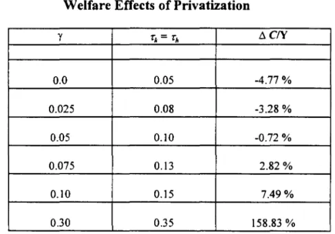
Table 2

Welfare Effects of Privatization

y _{Tk = Th} 6. CfY

0.0 0.05 -4.77 %

0.025 0.08 -3.28 %

0.05 0.10 -0.72 %

0.075 0.13 2.82%

0.10 0.15 7.49 %

0.30 0.35 158.83 %

Positive numbers mean a welfare cost - it is necessary to glve back, after

privatization, x% of consumption to agents in order to keep them as well off as they were

before privatization - while negative numbers mean a welfare gain, as consumption should

decrease for utilities to be equalized. Hence, according to the model simulations, if the true

value of gamma is less than 0.05 (actually, less than 0.055) society would benefit with

privatization. This gain is decreasing with gamma, which makes sense: for small gammas

the fact that the benevolent govemment takes the positive extemality due to G into

account when picking T is of minor importance when compared to the distortion

introduced to finance public investment.

Note that if the true gamma is 0.025 - a value estimated in a large number of

studies - the welfare gain is 3.28% of GNP, which is indeed very significant. As a

proportion of consumption, instead of GNP, it was ca1culated to be 4.89%. Taking the

consumption per capita in 1994 for the U .S. as being approximately 18.500 dollars, this

result implies that each individual would increase his/her consumption in the long °run,

after privatization, in 904.6 dollars a year. This numbers also mean that even making the

inefficiency and free supply to society of infrastructure services - privatization maybe

welfare improving and arguments against it based solely on under-investment are

incorrect, as this maybe the optimal action when the financing of public investment are

considered.

This result is however very sensible to parameters choice, specialIy gamma. If the

true gamma is 0.075, not far from some estimates in the literature - and welI below

Aschauer' s and Munnel' s estimates - society loses with privatization of infrastructure capital. In this case there is a welfare cost of2.82% ofGNP. Note also that the estimate of

welfare cost when garnrna is 0.30 is unrealistic high, one and a halftimes the GNP. This is

because the positive externality due to aggregate G

(G)

is so high that the gains from

public operation of infrastructure are huge - even taking into account that sizable

distortions are introduced in the economy, as optimal taxes rates are 0.35 - so that there is no question that govemment is more efficient in providing it.

If it is assumed that the tax structure is still more distorcive than the structure

above, the benefits from privatization increases. Suppose just as an illustration that public investment is entirely financed by capital taxo Although an extreme assumption, this idea

may capture the fact that in many countries, Brazil for one, savings, finance intermediation and even gross revenues are heavily taxed. We let alI other parameters remain the same

and repeated the experiment of table 2, which consists of estimating the welfare gains from

privatization when govemment chooses optimalIy tax rates. The results are displayed in table 3 below:

Table 3

Welfare Effects ofPrivatization (capital tax only)

y

_'k

!J.CN

0,00 0,11 -6.19

0,025 0,17 -5.63

0,05 0,21 -4.19

0,075 0,27 -1.92

0,10 0,31 1.17

The welfare gains from privatization in this economy where the tax structure is

more distorcive are much higher, as one could expect. For garnma equal to 0.025 the gains are now 5.63% of GNP, or 7.88% of total consumption, which arnounts to an increase of $1.458 dollars in the annual per capita consumption in the long run. At the sarne time,

welfare losses with privatization will only occur now for garnrnas above 0.091. It is also

shown in the table that when garnrna is 0.075, instead of a loss of 2.82% as in the previous case, there is now a gain of 1.92% of GNP. The reason for these results are simple, the

gains from intemalizing the positive extemality are now offset by higher distortions, so that you need higher extemalities ( garnrnas) for privatization to be welfare improving. Of

course, assuming a tax structure less distorcive (e.g., only tax on labor income) would

imply the opposite results and weaken the case of privatization.

5.3 Welfare effects of privatization with investment losses

Maybe the most popular argument favoring privatization is based on the supposed

inefficiency of public companies when compared to private counterparts. In a way or another, the idea is that those firms are not profit maximizing. They may operate according

to some political objective (inflation control or patronage), they may operate aiming to maximize the income of their employees or they may operate with higher leveIs of red tape

or employment. In all these cases operational costs are well above minimization leveI, so that society as a whole could gain ifthose firms are transferred to the private sector.

A tentative and simple way of modeling these inefficiencies is to suppose that

investment costs are higher in the public sector. There is informal evidence that this is in

fact the case, and the reason is not necessarily corruption but the very nature of govemment' s business and their relationship with the private sector. In a number of

countries in Latin America, for instance, private firms charge an over-price to govemment' s companies as an insurance against payment delay or default risk, two

common practices. In addition to that, most purchases from public companies has to be done through public bids and in general this is a long and bureaucratic processo Those

•

•

huge number of legal procedures that take time and cost money. For instance, the official

development bank of the Brazilian central govemment (BNDES) calculated that the

constmction of a hidro-eletrical plant they would finance for a public firm had its cost

dropped by half after it was transferred to private hands. The cost of investment projects of

a privatized steel mill in Brazil, in certain extreme cases, dropped to one third of its

original figures. The mIe of thumb, in Brazil at least, is that investment costs are at least

20% lower after privatization .

We modeled this fact in a very simple way. Suppose that instead of equation 7 we

have

(15)

so that a fraction lambda oftax revenues is lost and only (I-À.) is effectively invested. This

is equivalent to suppose that public investment is I /( l-À.) more expensive than private

investment. All the other features of the model, and the parameters values, are maintained.

We reproduced the privatization experiments of table 2, but now we want to know if

introducing investment losses in the public sector will imply in considerable larger gains

from privatization. In table 4 below, two values of lambda, 0.2 and 0.5, are used,

supposing moderate and high losses, and results from table 2 ( lambda equal to zero ) are

reproduced for the sake of comparison:

Table 4

Welfare Effects of Privatization with Investment Losses in the Public Sector

y flCfY

À=O À=0.20 À=0.50

0.00 -4.77 % -5.89% -8.17%

0.025 -3.28 % -4.99% -8.45%

0.05 -0.72 % -3.12% -7.91%

0.075 2.82% -0.37% -6.59%

0.10 7.49 % 3.31% -4.67%

•

•

•

The results above show that even a moderate investment 10ss may imply sizable

differences when considering privatization. If investment in the public sector is 25% more costly than in the private sector (lambda = 0.20) privatization is welfare improving for

gammas up to 0.075, a value in the upper bound of most estimates of this parameter. In

this case, a welfare loss of 2.82% of GNP is turned into a small gain of 0.37% after

assuming investment losses. Moreover, the gains are now much larger in the interval

where privatization is welfare improving: for gamma equal to 0.05, the welfare gains from

privatization increased more than 4 times.

As one could expect, in the extreme case of a very inefficient public sector - i.e.,

investment cost twice as large as in the private sector ( À = 0.5) - the case for privatization

is much stronger, even for high values of gamma. When gamma is 0.1, for instance,

society benefit from privatization is 4.67% of GNP or 7.5% of consumption. The

distortion introduced by the tax system and the high inefficiency of investment operations offsets the gains of internalizing the externaI effect of infrastructure capital, even for high

values of the externality parameter.

6 - Conclusion and Summary

It may seems that the model and its simulations left unanswered the basic question

it was supposed to answer: what are the allocation and welfare implications of privatization? However, this model economy, aIthough in certain dimensions highly

simplified, do deliver some lessons and intuitions that allow us to answer this questiono

The first lesson, also present in Devarajan et alli(l995), is that privatization can be welfare-enhancing in one country and welfare-decreasing in another, depending on the

relative importance of distortionary taxation and the positive externality due to

infrastructure. For instance, if we believe that the actual value of the sum of the externai and internai effect of public capital is on the lines of the estimates of Ferreira(l993),

Duffy-Deno and Eberts(l991), Canning and Fay(l993) and Baffes and Shah(l993) - who

•

hypothesis that favor the case of public provision of infrastructure, such as a benevolent

governrnent maximizing individuaIs' welfare, no operation inefficiency and free supply of

infrastructure services to society. However, if the actual value of the internaI and externaI effect of infrastructure capital is above these estimates then privatization is welfare

decreasing. Our simulations with capital income taxation only, on the other hand, showed

that for a given externality effect, the more distorcive the financing of public investment,

the higher the benefits from privatization.

A second conclusion is that, when inefficiencies in the public sector are allowed,

the case for privatization is considerable strengthened. And inefficiency is without

question a serious problem in the operation of public infrastructure operation. For instance, the World Bank(1994) estimates that timely maintenance expenditures of $12 billion

dollars would have saved road reconstruction costs of $45 billion in Africa in the past

decade, while informal evidence from Brazil showed that investment costs could drop to half after privatization. Although inefficiency was modeled in a very simple way, the

results from the simulations showed that the presence of even a small waste or overprice on investment can imply in sizable benefits from privatization. And would also increase

the set of economies (i.e., economies with larger externalities) that could benefit from it.

There are several ways we could extend this model. An immediate one is to

calculate welfare changes along transition paths and not only steady states, as temporary

losses may well offset long run gains when future is discounted. We could also drop the hypothesis of a benevolent governrnent and of free supply of infrastructure services and suppose that governrnent charges a fix price for it. Firms would take this price as given

and pick the profit maximizing leveI of g. Taxes would be levied in order to cover eventual

losses if prices charged were too low to cover costs, as it is often the case with public

servlces.

References

Aschauer, D., (1989) "Is Public Expenditure Productive?" Journal of Monetary Economics, 23, March, pp. 177 - 200.

v·---I

"

•

Baxter, M. and R. King, (1993) "Fiscal Policy in General Equilibrium " , American Economy Review, 83, pp. 315 - 334.

C anning , D. and M. Fay(1993) "The Effect of Transportation Networks on Economic Growth," manuscript, Columbia University.

Cooley, T. F. and G. D. Hansen (1989) "The Inflation Tax in a Real Business Cycle Model" , American Economy Review, 79, pp. 733 - 48.

Devarajan, Xie and Zou(1995) "Should Public Capital Be Subsidized or Provided?", Manuscript, World Bank.

Duffy-Deno and Eberts(1991), "Public Infrastructure and Regional Economic Development: a Simultaneous Equations Approach," Journal of Urban Economics, 30, pp. 329-43.

Easterly, W e S. Rebelo (1993) "Fiscal Policy and Economic Growth: an Empirical Investigation," Journal of Monetary Economics, 32, pp. 417-458.

Ferreira, P.C.(1993), "Essays on Public Expenditure and Economic Growth," Unpublished Ph. D. dissertation, University ofPennsylvania.

Grarnlich, E.M.(1994) "Infrastructure Investment: a Review Essay," Journal of Economic Literature, 32, pp. 1176-1196.

Hansen, G., e E. Prescott (1995)"Recursive Methods for Computing Equilibria of Business Cycles Models,"in Cooley. T. (org.) Frontiers of Business Cycle Research, Princeton University Press.

Holtz-Eakin, D. (1992), "Public Sector Capital and Productivity puzzle", NBER Working Paper no. 4122.

Hulten, C. and R. Schwab (1992), "Public Capital Formation and the Growth of Regional Manufacturing Industries", National Tax Journal, voI. 45,4, pp. 121 - 143.

Kydland, F. and E.C. Prescott (1982) "Time to Build and Aggregate Fluctuations",

Econometrica, 50, pp. 173 - 208.

Munnel, A.H., (1990) "How Does Public Infrastructure Affect Regional Economic Performance," New England Economic Review, September, pp 11-32.

_ _ _ _ _ (1994) "An Assessment of Trends in and Economics Impacts of Infrastructure Investment," in Infrastructure Policies for the 1990s, OECD.

Prescott, E.

c.,

(1986) "Theory Ahead of Business Cycle Measurement", Federal Reserve Bank of Minneapolis Quartely Review, 10, pp. 9 - 22.

______ and R. Mehra( 1980) "Recursive Competitive Equilibrium: the Case of Homogeneous Households," Econometrica, 48, pp 1356-79.

t,

1439298