REDUCING FALSE ALARM RATES DURING CHANGE DETECTION BY MODELING
RELIEF, SHADE AND SHADOW OF MULTI-TEMPORAL IMAGERY
Ben Gorte, Corné van der Sande
Delft University of Technology Geoscience & Remote Sensing Stevinweg 1, 2629 HS Delft, Netherlands
KEY WORDS:Change detection, Orthorectification, Rendering, Radiometry, Geometry
ABSTRACT:
Change detection on the basis of multi-temporal imagery may lead to false alarms when the image has changed, whereas the scene has not. Geometric image differerences in an unchanged scene may be due to relief displacement, caused by diferent camera positions. Radiometric differences may be caused by changes in illumimation and shadow between the images, caused by a different position of the sun. The effects may be predicted, and after that compensated, if a 3d model of the scene is available. The paper presents an integrated approach to prediction of and compensation for relief displacement, shading and shadow.
1 INTRODUCTION
The task addressed is validation of existing geoinformation using newer aerial imagery, whereby it is assumed that older imagery (used during creation of the information to be validated) is also available. The setting is about highly detailed, large scale topog-raphy in urban environments. Our experiments are at scales in the order of 1:1000 using aerial images of 3.5cm spatial resolution.
Validation is seen as the counterpart of object based change de-tection. The process tests the hypothesis concerning the validity of each object in an existing database against new data. Rejected objects require further investigation eventually leading to an up-date. Confirmed objects, on the other hand, will remain in the database unchanged, whereas the confidence in their validity in-creases. Our objective is making the validation process fully au-tomatic, in such a way that ’confirmed’ objects need no further in-vestigation. Therefore the omission error (of unnoticed changes) should be small. This usually comes at the cost of higher com-mission errors (false alarms), but clearly their number should be as small as possible too.
Change detection on the basis of multi-temporal imagery may lead to false alarms if (A) the scene has changed (and therefore also the image), but the changes are not relevant, or (B) the image has changed, but the scene has not. In both cases changes may be detected, although the existing information is still valid. Case (A) concerns, for example, moving cars, results of painting and gardening, falling leafs, wet vs. dry pavement etc. In the paper, however, we focus on (B).
Image differerences in an unchanged scene can be characterized as geometric or radiometric. Geometric differences are due to different camera positions, causing different relief displacements. The cure is true ortho image rectification, for which a digital sur-face model is required, which models, in addition to the terrain, buildings at level of detail (LOD) 1 or 2, as well as other 3d ob-jects, such as trees. Radiometric differences are caused by illu-mination changes due to the different dates and times of image acquisition. Assuming cloud free conditions these differences manifest themselves as shading and as shadow. Our purpose is to model these effects and try to perform radiometric normalisation of the imagery accordingly. Also this proces, like the true-ortho
Table 1: 3d Model parameters Area extent
min - maxx(RD) 154548 - 154900.11 min - maxy(RD) 462299.28 - 462648.33 min - maxz(NAP) 4.26 - 22.81 Number of triangles
terrain 81576
curbs 65607
walls 2104
roofs 9740
rectification, requires a 3d (surface) model describing the terrain and the objects in the scene.
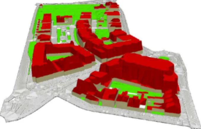
Figure 1: Automatic 3d reconstruction
We assume a DSM or 3d model to be available (Fig.1, Table 1), but part of the research is indeed about the required quality of this information for the purpose described. Note that at this stage it does not matter whether it is the same 3d information is being validated, or that this information is auxillary in the course of a 2d validation. In the latter case the required 3d data could, for ex-ample, be generated from the (old or new) imagery by matching, or by airborne laser scanning.
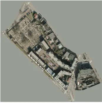
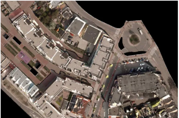
Figure 2: Masked areal image (2010)
per unit surface area depends on the sunlight direction. Assum-ing a (locally) flat surface, this amount is maximum when the normal vector of the surface points exactly towards the sun, and decreases with cos(ϕ) as the angleϕbetween the normal vector and the sun vector increases. The amount of reflected light, as re-ceived by the imaging sensor, strongly depends on the amount of incident light. Assuming Lambertian reflectance the intensity of the reflection from a given surface patch at the sensor is indepen-dent of the sensor position. It linearly depends on the product of incident intensity and reflectivity, whereby the latter is constant in an unchanged scene. In addition to directly incident sunlight, the scene receives diffuse light, coming from all directions out of the blue sky. Its intensity at a certain surface patch is sometimes modeled as the portion of the hemispere that is visible from that patch (but we will not pursue this in this paper).
Shadow occurs if direct sunlight is not reaching certain parts of the scene, because it is blocked by other (non-transparent) ob-jects, which are located between the sun and those shadowed parts. These parts do receive scatterred, diffuse light from the blue sky, and possibly also from reflections at other nearby ob-jects. The indirect light that illuminates shadowed areas is indeed more blueish than direct sunlight. Note that directly-illuminated objects receive scattered light as well.
The emphasis of the paper is on modelling shadow and shading in order to get an estimate of the illumination at each surface visible in an image at the time the image was recorded. The algorithm renders a 3d model, which is represented as a TIN, into a 2d ver-tical view raster dataset with a spatial resolution matching the available imagery. A complication in our case is the size of the resulting datasets: the number of pixels of an aerial photograph is a few orders of magnitude larger than that of a computer screen. In addition, the original aerial photograph itself is true-ortho rec-tified using the same 3d datamodel, into the same resolution as the rendering. After that it is possible to ’normalize’ the images, eliminating radiometric differences from multi-temporal imagery and reduce the false-alarm rate at unchanged objects. Working ’object based’ on the basis of a 3d model allows for taking the accuracy and detailedness of the model, and the possible errors in shading, shadowing and orthorectification resulting from it, into account when deciding about the validity of each object.
Table 2: Aerial Photographs
Image 2010 2011
Camera Vexcel UltraCam-Xp Sensor size 17310 x 11310 pixels
Pixel size 6 x 6µm
Principal distance 105.0 mm Exterior Orientation
Xo 154697.55 154705.76
Yo 462473.45 462473.90
Zo 623.74 581.78
ω(gon) -0.4754 0.0313
ϕ(gon) 0.3008 -0.1212
κ(gon) -99.166 -99.5445
Sun position determinaton
Date Mar 8 2011 Apr 23 2010 Time of day (UTC) 10:27:32 AM 9:46:21 AM
Longitude E 5.38 E 5.38
Lattitude N 52.15 N 52.15
Altitude 5m 5m
Sun Azimuth angle 59.654 45.366
Sun Zenith angle 156.22 140.53
2 AVAILABLE DATA
The 3d model (Fig. 1) used in the experiment below is located in the center of the city of Amersfoort in the Netherlands. It was cre-ated from a combination of large scale 2d topographic data (the Dutch BGT dataset) and a laser altimetry point cloud. The point cloud is part of the Dutch AHN-2 dataset, which was set up by the National Survey Department and the regional Water Boards, mostly for water management purposes. It is a high density (on average more than 20 pts/sq.m.) point cloud, in which terrain points and ’object points’ (buildings, trees etc.) are separated, with systematic error below 6cm, and random error below 6cm as well. The buildings in the model were reconstructed fully au-tomatically by software of Sander Oude Elberink according to his methodology in (Oude Elberink, 2010), in the context of an ur-ban hydrology project (Verbree e.a. 2013). The streets, including curbstones, play a major role in urban hydrology; therefore they are represented with great detail (see Table 1). The sub-model used here is located in a 350x350m square, which, however, is not fully covered by the model (Fig. 2).
The two aerial photographs used in the experiments cover the area of the 3d model. They are part of yearly campaigns flown over the Netherlands, in this case from 2010 and 2011. Red, green and blue channels are available; the ground resolution is about 3.5 cm. The 350m area extend of the 3d model, therefore, require images size of around 10000 x 10000 pixels.
3 ALGORITHMS
The goal of the following section is to remove the effects of relief displacement, as well as of shadow and shading, from aerial im-ages, in order to make these images better comparable in a change detection context.
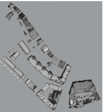
Figure 3: Building (roof) objects 2010
which will be generally described here, before going to the de-tails of the algorithm. TIN to grid conversion is the projection of a 3d triangulated model onto a 2d plane, sampled regularly into a grid. The sampling space in the model coordinate system de-termines the grid resolution. The process works as follows: first, an empty grid is constructed on the basis of the size of the pro-jected area (the minimum and maximum X and Y coordinates) and the wanted resolution. Next the process works one triangle at a time. A bounding box around the projected triangle deter-mines the candidate grid cells for this triangle. Which grid cells are actually involved is decided by submitting each of them to a point-in-triangle test.
Figure 5: Roofs (detail) 2010
Figure 4: Building (roof) objects 2011
Figure 6: Roofs (detail) 2011
Also 3d rendering, which is the visualisation of a triangulated 3d model into an image on a computer screen, can be considered TIN to grid conversion. A camera position is assumed inside the model. This is the projection center, and the projection plane is perpendicular to the camera axis at a distancef(the focal distance of the camera) from the projection center. The grid positions will correspond to the image pixels. While doing the conversion for a certain triangle the distances between the selected grid cells and the camera are computed. It will occur that a single grid cell is involved in the conversion of more than one triangle. Now only the triangle closest to the camera should influence the rendering; all the others are “hidden”. In a so-called Z-buffer this distance is recorded for every grid position. If a closer triangle comes along the Z-buffer is updated; results for farther triangles are simply discarded.
Figure 7: True ortho (detail) 2011; note the double roof edge at the building to the right, due to occlusion.
3.1 True-ortho rectfication
Change detection will be carried out in an object based fashion: each object in the geo-database is considered a hypothesis, and is evaluated against the image content. Of particular relevance is the question whether the support for an hypothesis has decreased between the older and the newer image. Therefore it is neces-sary that an object is covered by exactly the same portion of ei-ther image, irrespective of the object being at terrain level (e.g. streets, gardens, parking lots) or above terrain (e.g. buildings, tree crowns).
The standard way to accomplish this with areal images is by true-ortho rectification. This is a vertical projection of the TIN 3d model onto the (X,Y) plane, which is then sampled into a regular grid. The projection center is at infinite height. For each grid cell, sampled at coordinate (Xp,Yp) in the projection plane, the Zp value can be found, according to the model, at the surface that is visible in the image. By using the exterior orientation parameters of the aerial image the pixel position in that image is known, and the value at that pixel can be copied into the current grid cell of the ortho image.
When using images of different epochs in a change detection con-text, the above will ensure that the correct sets of pixels will be assigned to each object. It is possible the generate a grid for the entire model (all visible objects), or for selected objects only. In Fig. 3 and 4 only roof objects, as seen in both images, are shown, and can be compared one by one in a change detecton algorithm. A detail of both images is show in Fig. 3 and 3. Note that at cer-tain (X,Y) positions the “top” object in the model is not visible in the image due to occlusion. There, the value in the ortho-image is wrong, as in Fig. 7. The entire roofs are correct, but the occluded part of the terrain immedately next to the building is shown incor-rectly (by repeating the roof pixels); the alternative would have been to put theunknownvalue at those places.
3.2 Shadow and Shading
Predicting shadow and shading in an ortho image of a 3d model can be described as a TIN to grid conversion as well. The pixel value at a certain grid position is now determined by the question whether that position receives direct sunlight. If the answer is no, it is a shadow pixel, and if it is yes, the incidence angle of the sunlight onto the surface facet given by the triangle in the model determines the shading.
The process knows the position of the sun during the image record-ing from the lat-long location of the scene and the data and time
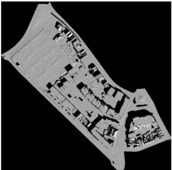
Figure 8: Simulated shade and shadow 2010
Figure 9: Simulated shade and shadow image 2011
of the acquisition. We compute this position (i.e. the azimuth and zenith angles) using the algorithm of Reda and Andreas (2003) in the implementation of Vincent Roy (2009), made available through the Matlab Central.
Introducing cast shadows into rendering is a non-trivial, however solved, problem in computer graphics. Chris Bentley (1995) de-scribes two alternatives, (a) using Z-buffering (Algorithm3.2) and (b) using Ground transformation. Our algorithms is modified Z-buffering (Williams, 1978), having both camera and light source at infinite distance (Blinn 1988).
Algorithm 1Z-buffering (Bentley 1995) Implementation of Shadow Z-buffer Algorithm Precomputing phase
1.0 for each light source
1.1 make light point be center of projection 1.2 calculate transformation matrices 1.3 transform object using light point matrices 1.4 render object using zbuffer - lighting is skipped 1.5 save computed zbuffer (depth info)
Object rendering phase
2.0 make eye point be center of projection 3.0 recalculate transformation matrices 4.0 transform object using eye point matrices 5.0 render object using zbuffer
5.1 for every pixel visible from eye
5.1.1 transform world point of pixel to shadow coordinates 5.1.2 for every light source
5.1.2.1 sample saved zbuffer for that light 5.1.2.2 if shadow coordinates < zbuffer value 5.1.2.2.1 pixel is in shadow
shadow information.
A benefit is that shading information is obtained "on the fly" when modelling shadow: in the rotated model of phase 1 the angle between the normal vector of a triangle (from the plane equa-tion given by the three vertices) and the sun vector, which equals (0,0,1), is easily computed and stored with the triangle list. Dur-ing phase 2 the cosine of this angle is used as the output value in the shading image. Note that shading computation at non-flat building roofs requires an LOD2 building model.
3.3 Shadow and shading compensation
Sun-lit surfaces in the scene receive both direct and indirect (dif-fuse) illumination. Radiation from the sun in cloud-free wheather circumstances partly travels to the earth surface in straight lines (if we ignore refraction). Another part is absorbed by the atmo-sphere, and yet another is scattered. The effects of absorption and scattering are wavelength-dependent. Absorption happens at very specific wavelengths, called absorption bands. Scattering, including the Raleigh scattering considered here, is a broad-band phenomenon; it is stronger, however, as wavelengths get shorter, and therefore in the visible range of the spectrum blue light is scattered more than green and red (to mention just a few). There-fore the sky is blue and, moreover, the illumination at shadowed parts of the scene is, apart from being weaker, contains a rela-tively large amount of ’blue’, compared to the solar spectrum. Consequently, in the directly-illuminated parts of the scene the light contains a slightly larger (relative) amount of green and red, compared to the solar spectrum (which is rarely corrected for, however).
The purpose of modelling shadow, in this paper, is to find out which pixels in the true-ortho rectified image are directly illumi-nated and which ones are in the shadow. If we take the former ones as ’correct’, the shadow effect at the latter can be compen-sated by multiplying their pixel value by a factor that depends on the estimated ratio between direct and diffuse illumination. In or-der to account for wavelenth dependency, different factors could be applied for the red, green and blue image channels. Thanks to the excellent radiometric resolution of nowaday’s digital cameras also shadowed parts of the scene have sufficient contrast to make this multiplication work.
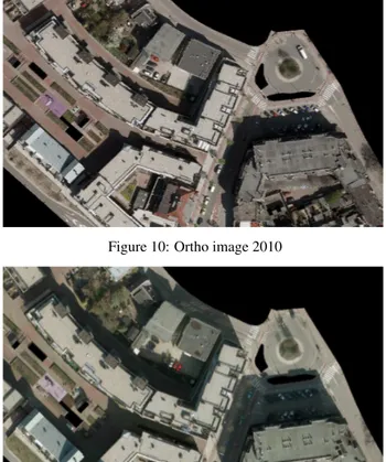
Figure 10: Ortho image 2010
Figure 11: Ortho image 2011
Shading
The amount of direct illumination at sun-lit surfaces is propor-tional of the cosine of the angle between the surface normal and the sun vector. With a zero-angle (the surface being perpendicu-lar to the soperpendicu-lar rays), the intensity is maximum, gradually going down to 0 as the angle tends to 90 degrees. The cosine was com-puted during phase 1 of the shadow algorithm, and stored in the shading image during phase 2.
The amount of diffuse illumination, in a first approximation, can be considered the same in all cases, as diffuse light is coming from all directions. Therefore, the total illumination at a surface can be computed as a constant (for the diffuse component) plus a variable amount, as given by the shading image. The constant is equal to the factor, applied above, for shadow compensation - the shadows have value 0 in the shading image.
4 RESULTS AND DISCUSSION
The above-described algorithms for true-ortho rectification and shadow/shading estimation and compensation are applied to the two Amersfoort images of 2010 and 2011. The variable amount of direct illumination (on a scale of 0-255) was estimated in shad-ing images (Fig. 8 and 9). The shadowed areas in those images have value 0 (black). Fig. 8 has a generally brighter appearance than Fig. 9. This is not an error, as the corresponding aerial im-ages are from end of April vs. beginning of March. Therefore the sun is higher in the first, leading to more intense illumination. On the same scale the amounts of (constant) diffuse illunination was estimated as 80, 90 and 100 for red, green and blue respectively.
Figure 12: Shading/shadow compensation 2010
Figure 13: Shading/shadow compensation 2011
and 11. Unfortunately also some defects are visible, such as the bright areas to the North and East of some of the buildings. These are caused by incorrectly handling the effect of occlusions men-tioned earlier. Also there are some sun-lit tree crowns above shad-owed parts of the terrain surface; those tree crowns are incorrectly ’compensated’. Conversely, shadows cast by trees are not mod-elled, as there are no trees in the model. Therefore compensation at these shadowed areas did not take place.
5 CONCLUSION
The paper presents a integrated method to account for effects oc-curing in areal imagery due to the 3d nature of urban scenes. These effects are relief displacement, shadow and shading. To consider those effects is highly relevant during change detection, as they may manifest themselves differently in subsequent im-ages, due to differences in camera position and Sun position. This may lead to false detection of changes. Increasingly available 3d information in urban environments may be used to predict those effects, leading to the opportunity to compensate for them on the basis of estimates of the ratios between direct and diffuse illumi-nations, also depending on the wavelength.
The next step in our research will be to investigate whether the corrected imagery indeed leads to improved change detection. Meanwhile we will study the extend to which the quality of 3d models influences the results. Lastly, we want to include other objects than buildings, such as trees, in the approach.
REFERENCES
Bentley, Chris (1995), Two Shadow Rendering Algorithms, http://web.cs.wpi.edu/~matt/courses/cs563/talks/shadow/
shadow.html
Blinn, James (1988), "Me and my (fake) shadow", IEEE Com-puter Graphics and Applications, January 1988.
Maren, Gert van and Jinwu Ma (2012) , 3D Analyst – Feature & Volumetric Analysis, Esri International User Conference, San Diego, July 2012.
Oude Elberink (2010), S, Acquisition of 3D topography: auto-mated 3D road and building reconstruction using airborne laser scanner data and topographic maps, PhD. Thesis, University of Twente, 2010.
Reda, I., Andreas, A. (2003) Solar position algorithm for so-lar radiation application. National Renewable Energy Laboratory (NREL) Technical report NREL/TP-560-34302.
Roy, Vincent (2009) , http://http://www.mathworks.com/ matlabcentral/fileexchange/4605-sunposition-m, accessed 28 March 2014.
Verbree, E, M de Vries, B Gorte, S Oude Elberink, G Karimlou (2013) , Semantic 3D city model to raster generalisation for water run-off modelling, SPRS Annals of the Photogrammetry, Remote Sensing and Spatial Information Sciences, Volume II-2/W1.