Hierarchical Bayesian Spatio
–
Temporal
Analysis of Climatic and Socio
–
Economic
Determinants of Rocky Mountain Spotted
Fever
Ram K. Raghavan1,4*, Douglas G. Goodin2, Daniel Neises3, Gary A. Anderson1, Roman R. Ganta4
1Kansas State Veterinary Diagnostic Laboratory, Department of Diagnostic Medicine and Pathobiology, Kansas State University, Manhattan, Kansas, United States of America,2Department of Geography, Kansas State University, Manhattan, Kansas, United States of America,3Bureau of Epidemiology and Public Health Informatics, Kansas Department of Health and Environment, Topeka, Kansas, United States of America,4Center for Excellence in Vector Borne Diseases, Department of Diagnostic Medicine and Pathobiology, Kansas State University, Manhattan, Kansas, United States of America
Abstract
This study aims to examine the spatio-temporal dynamics of Rocky Mountain spotted fever (RMSF) prevalence in four contiguous states of Midwestern United States, and to determine the impact of environmental and socio–economic factors associated with this disease. Bayesian hierarchical models were used to quantify space and time only trends and spatio– temporal interaction effect in the case reports submitted to the state health departments in the region. Various socio–economic, environmental and climatic covariates screeneda
pri-oriin a bivariate procedure were added to a main–effects Bayesian model in progressive steps to evaluate important drivers of RMSF space-time patterns in the region. Our results show a steady increase in RMSF incidence over the study period to newer geographic areas, and the posterior probabilities of county-specific trends indicate clustering of high risk counties in the central and southern parts of the study region. At the spatial scale of a county, the prevalence levels of RMSF is influenced by poverty status, average relative humidity, and average land surface temperature (>35°C) in the region, and the relevance of these factors in the context of climate–change impacts on tick–borne diseases are
discussed.
1. Introduction
Rocky Mountain spotted fever (RMSF) is a life–threatening fulminant tick-borne infection caused by the obligate intercellular bacteriumRickettsia rickettsii(Family: Rickettisiaceae, Order: Rickettsiales) [1]. This disease has been reported from most of the lower 48 states in the United States, with onsets typically occurring during the tick season (April through September)
OPEN ACCESS
Citation:Raghavan RK, Goodin DG, Neises D, Anderson GA, Ganta RR (2016) Hierarchical Bayesian Spatio–Temporal Analysis of Climatic and
Socio–Economic Determinants of Rocky Mountain
Spotted Fever. PLoS ONE 11(3): e0150180. doi:10.1371/journal.pone.0150180
Editor:Shannon L. LaDeau, Cary Institute of Ecosystem Studies, UNITED STATES
Received:November 20, 2015
Accepted:February 10, 2016
Published:March 4, 2016
Copyright:© 2016 Raghavan et al. This is an open access article distributed under the terms of the Creative Commons Attribution License, which permits unrestricted use, distribution, and reproduction in any medium, provided the original author and source are credited.
[1–3]. Despite the name, most RMSF cases occur in the lower Midwest and southern United States, with the states of Oklahoma, Arkansas, Missouri, Tennessee, and North and South Car-olinas reporting most cases per year [4]. The disease is difficult to diagnose since symptoms do not develop until a few days well into infection [5], [6], and a lack of early treatment could lead to death [7]. Young children and the elderly are more frequently affected by RMSF [8], and although case fatality rates have declined during the last decade the incidences of RMSF has increased during the same time period in the United States [9].
Increased incidence of vector–borne diseases could be at least partly due to ongoing cli-mate–change [10–12], and there is considerable interest in attributing climate–change effects on disease incidences. Arthropod life–cycles are highly regulated by climatic conditions, and the changes in recent climate patterns due to climate–change could affect incidences of tick-borne diseases in many ways. Some of these include changing spatial distribution of ticks and tick-borne pathogens [13], [14], and the persistence and replication rates of tick pathogens in their hosts [15]. Influential climatic factors behind increased incidence of RMSF are not clearly understood but are worth considering under a climate–change context.
At least three different tick species are confirmed vectors of RMSF in the United States [3], [16]. The population dynamics and spatial range of these ticks along with those of other arthro-pods may have changed in the past decade [17], [18] as a result of climate–change and other anthropogenic influences. The primary tick that transmitsR.rickettsiito humans east of the Rocky Mountains is suggested to be the American dog tick,Dermacentor variabilis[3], although the role ofD.variabilisticks in the transmission has been contested since several recent reports have not detected the pathogen among field-collected ticks or those that were attached to humans or animals [19], [20]. The Rocky Mountain wood tick,D.andersoniis implicated in transmissions in the Rocky Mountain States and in the Pacific west. And, the brown dog tick,Rhipicephalus sanguineushas been shown to transmit this bacterium in the southwestern United States and along the United States–Mexico border [3], [21].
Determining the associations of influential climate and/or short–term weather factors with vector–borne diseases are problematic since they are often confounded with the effects of phys-ical environment and socio–economic factors [10], [22]. A number of studies have shown rela-tionship between various climatic (temperature, rainfall, humidity) factors and tick-borne illnesses but also physical environmental (land cover, landscape structure) and socio–economic factors [23], [24]. Therefore, attempts to determine climate associations with infectious dis-eases may benefit by simultaneously considering these additional factors. Also, abiotic determi-nants of vector–borne diseases are subject to changes due to influences of varying spatio–
temporal factors, and incidences of vector–borne diseases have strong spatio–temporal depen-dencies, which necessitates evaluations of any associations to be conducted in a spatio– tempo-ral context [25], [26]. Bayesian spatio–temporal models provide a flexible and robust platform for space-time analysis and also for evaluating covariate association with disease incidences between aggregated areal units such as a county. Such models have been used to study other tick-borne disease systems at a county scale [27], [28].
The purpose of this study was to evaluate the spatio–temporal pattern of RMSF incidence in the central United States spanning four contiguous states (Kansas, Missouri, Oklahoma and Arkansas) where this disease has noticeably increased over the past decade. Using case reports submitted to the respective state health departments over the years we asked the following spe-cific questions; Is there an overall trend (increase, decrease or stable) for RMSF in the region comprising these four states? Are there areas within the region where there are the departures from the overall trend, or specifically high‘risk-areas’? And, what are some of the influential factors–including any climate–change indices that are associated with RMSF incidence in this region?
Health (501 280-4433), and Oklahoma State Department of Health (405 271-5600) directly with data requests. The lead author requested data for this study from these departments using the telephone numbers provided.
Funding:This study was supported in part by the PHS grant number AI070908 from the National Institute of Allergy and Infectious Diseases, National Institutes of Health, USA. This article is a contribution (Contribution no. 16-222-J) from the Kansas Agricultural Experiment Station. Publication cost for this article was provided by the K-State Open Access Publishing (KOAPF) program. The funders had no role in study design, data collection and analysis, decision to publish, or preparation of the manuscript.
2.0 Materials and Methods
2.1 Study area
The spatial extent considered in this study included the contiguous states of Kansas, Missouri, Oklahoma and Arkansas in central United States, which have recorded RMSF cases since the first identification of the disease, and has some of the highest number of incidences in the United States. Climate in the study area is transitional from east to west, and as well as south to north, with the southeastern region receiving progressively more rainfall than the west.
2.2 Data
2.2.1 Ethics statement. The RMSF data used in this study was notifiable by individual state health departments to the Centers for Disease Control and Prevention (CDC), and were aggre-gated annually to their respective administrative units. No individually–identifiable information was collected for this study. The use of RMSF data was approved by the Internal Review Board at Kansas State University’s Office of Research Compliance (IRB #7465) and the study was con-sidered exempt from the requirement for full review by the Missouri Department of Health and Senior Services (MDHSS) Institutional Review Board based on 45 CFR 46.101(b)(4).
2.2.2 Epidemiological data. Annual county–level RMSF cases between years 2005 and 2014 were obtained from the state health departments of Kansas, Missouri, Arkansas and Okla-homa. Cases are classified into‘confirmed’,‘probable’, and‘suspected’categories per CDC guidelines. Case classification for RMSF changed once during the study period in 2008 and included the‘suspected’criteria for diagnosis. For the purposes of this study all three categories were considered to indicate positive RMSF diagnosis. In the case of Missouri, cases were pre-dominantly aggregated at county–level; however, they also included three additional public health administrative units that were subsequently used in the disease mapping and Bayesian spatio–temporal analysis. Population data for these jurisdictions were provided by the MDHSS, and for all other jurisdictions an average value of county population recorded for years 2000 and 2010 by the US Census Bureau was used.
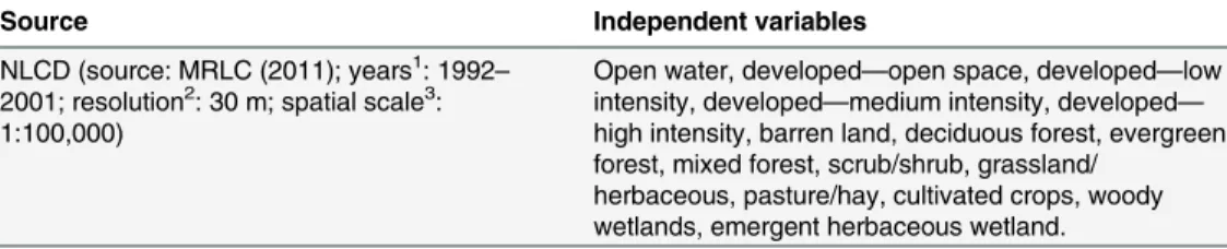
2.2.3 Covariate data. Covariate data for this study was collected from three thematic groups; viz., physical environment, climate, and socio–economic status. For environmental data, the percentage land occupied by different cover types in each county was estimated in a geographical information systems (GIS) environment from the publicly available 2006 National Land Cover Dataset [29] (Table 1). Among climate variables, county averages of annual mean temperature; the maximum normalized vegetation index (NDVI); minimum
Table 1. Physical environment variables screened in the study.
Source Independent variables
NLCD (source: MRLC (2011); years1: 1992
–
2001; resolution2: 30 m; spatial scale3: 1:100,000)
Open water, developed—open space, developed—low
intensity, developed—medium intensity, developed—
high intensity, barren land, deciduous forest, evergreen forest, mixed forest, scrub/shrub, grassland/
herbaceous, pasture/hay, cultivated crops, woody wetlands, emergent herbaceous wetland.
1Years represent the time period during which satellite images of land cover were captured for creating the data set, including multiple images within a year.
2Resolution indicates the
fineness of ground data as captured by a satellite image, shorter resolution meaning higher clarity;
3Spatial scale indicates the scale for which interpretations are appropriate.
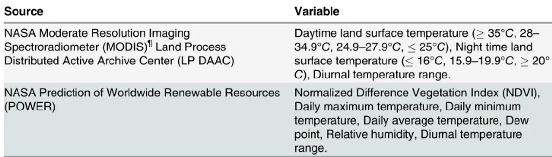
land surface temperature (LST); mean LST; precipitation and relative humidity were extracted in a GIS environment for the corresponding years. The LST and NDVI estimates were derived from MODIS (Moderate Resolution Imaging Spectroradiometer) imagery [30]. Precipitation and relative humidity were derived from the Prediction of Worldwide Renewable Energy (POWER) web portal of the NASA Langley Research Center [31] (Table 2). Climate variables were extracted for a period roughly corresponding to the active tick–season in the region (May through August). For socioeconomic variables, the U.S. Census 2010 data on population and housing were obtained from the National Historical Geographic Information System (NHGIS), a publicly available online resource for U.S. Census Bureau’s historical and current population data [32] (Table 3). Identical census attribute information and geographic bound-ary files for counties were also obtained from the NHGIS. From the tables, 20 housing and 23 population related variables were extracted for each county by spatial query and joined to the census shapefiles using the common GIS codes.
2.3 Statistical analysis
2.3.1 Covariate selection. Candidate explanatory variables to be included in the Bayesian hierarchical models were screeneda prioriin order to avoid model fitting issues. Several fre-quentist bivariate regression models were used to evaluate each variable independently and only variables that were significant at a liberalp0.2 were kept for further analysis. A bivariate regression takes the form,
ðYijÞ ¼b0þ bkvkij:
whereYijis RMSF relative risk,β0the intercept coefficient, andβkthe coefficient for the
explan-atory variablevkij(k=1,. . .,n) and (i= 1,. . ., 105county;and j=year2005,. . ., 2014). Care
was taken not to remove candidate variables that were deemed clinically relevant [33]. Among screened variables the presence of multicollinearity was tested by estimating the variance infl a-tion factor (VIF) and all variables with a (VIF10) were considered to indicate multicollinear-ity, in which case, one of the variables was dropped at a time until multicollinearity was absent. Non–linearity among independent variables was evaluated, and significant variables with non–
linearity were categorized using cutoffs based on scatter–plots.
2.3.2. Bayesian model specification. The observed number of RMSF cases in the study was notated asYijamongNijindividuals at risk in the population of countyi, diagnosed with
Table 2. Climate variables evaluated in the study.
Source Variable
NASA Moderate Resolution Imaging Spectroradiometer (MODIS)¶Land Process Distributed Active Archive Center (LP DAAC)
Daytime land surface temperature (35°C, 28–
34.9°C, 24.9–27.9°C,25°C), Night time land
surface temperature (16°C, 15.9–19.9°C,20°
C), Diurnal temperature range. NASA Prediction of Worldwide Renewable Resources
(POWER)
Normalized Difference Vegetation Index (NDVI), Daily maximum temperature, Daily minimum temperature, Daily average temperature, Dew point, Relative humidity, Diurnal temperature range.
¶Several sixteen day composite MODIS images were downloaded for each year, for a period
corresponding roughly to the tick season in North America (March–September), and county–level averages
were estimated for different variables using pixels completely present within independent county boundaries.
RMSF in yearj.Yijwas assumed to follow a Poisson approximation, (Yij) ~Poisson(Eijθij),
whereEijis the expected number of the population at risk for RMSF andθijis the relative risk.
Although a Binomial approximation could have been used in this context sincenis known, rel-atively only few RMSF infections occur randomly over time with different age groups, whose members vary throughout the study period due to aging; therefore, Poisson distribution was chosen over Binomial since the latter assumes constant population of individuals. And, since RMSF prevalence is disproportionate among different age groups [4], standardized rates were calculated assuming five age classesl, (<5, 5–19, 20–45, 46–65 and>65). Mapping crude
rates can be non–informative or misleading when population in some areal units are small, resulting in large posterior estimates, which in turn render it difficult to distinguish chance var-iability from genuine differences. The expected number of RMSF cases was therefore calculated by
Eij¼
X
l nijl
X
i
X
ijlYijl
X
i
X
ijlNijl
:
A logit link function in an extended generalized linear model (GLM) structure was used that incorporated stochastic spatial and temporal functions and as well as different covariate effects. We first fitted a parametric spatio–temporal model with various random terms to act as surrogate indicators of unobserved risk factors that vary over time, space or both. In a second model, the parametric terms were replaced with nonparametric terms to assess any model improvements. In a third step, we extended the second model with different covariates to explain spatio-temporal patterns.
The parametric model was notated as following,
LogðyijÞ ¼aþuiþviþgjþCij:
Where,α(intercept term) represents the mean prevalence of RMSF in all counties in all years, Table 3. Population and housing variables evaluated in the study.
Census category
Independent variables£
Housing Housing units(total housing units),Tenure(owner occupied, renter occupied),Tenure
(Historic or Latino Householder)(owner occupied, renter occupied),Race of
householder(white alone, Black or African American alone, Asian alone),Household
size(1–person, 2–person, 3–person, 4–person, 5–person, 6–person, or 7–more person
household),Year structure built(Built 2005 or later, 2000 to 2004, 1990 to 1999, 1980 or earlier¶). (20 variables).
Population Population(total population),Race(White alone, Black or African American alone, Asian alone),Household income in the past 12 months(Less than $10,000, $10,000 to $14,999, and thirteen other variables representing $49,999 incremental income thereof up to $199,999, and $200,000 or more),Poverty status in the previous 12 months
(income in the past 12 months below poverty level, income in the past 12 months at or above poverty level). (23 variables).
Definitions of different census variables can be found from their source (NHGIS) website at:https://www. nhgis.org/.
£Observations for all the independent variables are counts, in continuous form, and recorded per areal unit (county). Items in italics are Census Table names, and items within parenthesis are independent variables evaluated in this study.
¶The variable 1980 or earlier was derived by summing all the number of houses built prior to 1980 originally available infive–year increments in census.
anduiandviare random terms accounting for spatially structured variation in RMSF
preva-lence and unstructured heterogeneity, respectively. No interaction was assumed to exist betweenuiandvi, and these terms were assignedui~CAR, andvi Normalð0; s
2
vÞpriors. Spatial dependence inuiwas applied by assuming a conditional autoregressive model (CAR)(γ)
with a Gaussian distribution, which implies that eachuiis conditional on the neighborujwith
varianceðs2
iÞdependent on the number of neighboring countiesniof countyi, i.e.,
uiju;j neighbor of iN
1
ni
gXni
j¼1uj; s2
i ni
:
Theγjterm measured the purely temporal and a linear time trend in the data, which assumed no temporal structurea priori. An independent mean–zero normal prior with unknown vari-ances2
gwas used forγ. In the same model, in order to account for spatio–temporal interaction
effects in RMSF prevalence, a spatially structuredCijterm modeled as an intrinsic Gaussian Markov randomfield (IGMRF) [34] was included, with a joint prior density forψ= (ψ1,. . .,ψI)T
written as
pðcjs2
cÞ / exp
1
2s2
c
X
ii0
ðci ci0Þ
2
" #
:
A major limitation with the above described model is the assumption that there is a linear time trend in each region. Therefore, in a second model the linearity assumption was dropped and a nonparametric term,βjwas included, whose prior density can be written as
pðbjs2
bÞ / exp
1
2s2
b
XT
t¼2
ðbt bt 1Þ
2
" #
:
Theβterm quantified the overall time trend for the region. In addition, a nonparametric Type–IV interaction prior [25], [35] was assigned to theCijterm, which is notated as
pðcjs2
cÞ / exp
1
2s2
c
XT
t¼3 XI
ii0
fðcit 2c
i;t 1þci;t 2Þ ðci0;t 2 2ci0;t 1þci0;t 2Þg 2
" #
:
For the extended models with covariate terms, different covariates were included to the sec-ond model in several steps, starting with a model that included all covariates screened in the bivariate procedure that retained significance at a liberal (p0.2) value followed by the removal of one variable at each step. Individual covariates were retained in the model unless their removal resulted in the increase of Deviance Information Criterion(DIC)value by 5 units or more. The removed covariates did not re–enter the model and all covariates were assigned noninformative priors,Normalð0; s2
vÞ:
The spatiotemporal interaction term,Cijin the covariate model measured the trend after
accounting for purely spatial (α+ui+vi) and purely temporal effects (βij) in addition to the
covariate effects, and reveals the variation in RMSF incidence trends across counties over time. The differential trend (the difference between overall trend and local trend) of a countyifor a given yearjcan also be estimated fromCij, withCij>0 indicating steeper than overall trend
andCij<0 indicating a less steeper the overall trend. Counties whereCij= 0 are areas where
the trends are equal [36].
models that consider many random effects [38]. Thus, in addition toDICtheLSof each model was computed to assess predictive quality of models [39], [40], which is represented by
LS=−log(πij), whereπij=pr(Yij=yij|y-ij) denotes the cross-validated predictive probability.
A smallerLSindicates better predictive quality of a model.
All model posterior parameters were estimated using a Bayesian framework implemented using R–INLA software [41], and the median estimates from the posterior distribution and their corresponding uncertainty measures [95% Credible Intervals (CrI)] were recorded.
3. Results
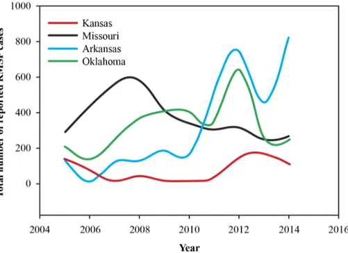
From January 1, 2005 to December 31, 2014, there were a total of (n= 11,062) confirmed, prob-able and suspected cases of RMSF reported to the health departments of the four states included in the study. Missouri recorded the most number of cases (n= 3,766) followed by Arkansas (n= 3,271) and Oklahoma (n= 3,271), and Kansas recorded the least number of cases (n= 754) among the four states during this period. Throughout the study period, and in all four states males were diagnosed at a higher rate than females, with a male female ratio averaging 2.2:1 for all states. Also, the disease was more common among the 46–64 year old age group followed by the65 year old age group. A plot of case numbers in the four states during the study period is illustrated inFig 1. A general upward trend for cases can be observed for Arkansas and Okla-homa, while in Missouri the case numbers have fallen since 2007–2008 period with only a small increase in 2014, and Kansas is largely constant throughout the study period. Also, with the exception of Missouri, all three states have recorded a marked increase in the number of cases during the year 2012. Missouri experienced a similar peak in the year 2007.
Of all the variables evaluated in the bivariate screening procedure in this study, five retained significance at a liberalp0.2 level (Table 4). Two variables,“Year structure built in 2005 or later”and“Year structure built in 2000–2005”were revealed as collinear among the selected var-iables. Non–linearity was not observed among the selected variables. Numerical results of
Fig 1. Plot of reported number of cases submitted to different state health departments in the study region.
Bayesian hierarchical models, the posterior Bayes median estimates and their corresponding 95% CrI are present inTable 5. FromTable 6, we see that Model–1 has the highest deviance information criterion (DIC) value pointing to the presence of additional space–time structure to the data beyond just purely spatial and temporal main effects. The addition of nonparametric terms to the fixed effect spatio–temporal model markedly reduced theDICvalues, and the sub-sequent addition of covariate terms further improved the spatio–temporal model performance.
‘Income in the past 12 months below poverty level’(henceforth, poverty–status),‘average rela-tive humidity’and‘average daytime land surface temperature35°C’were retained in the final, best fitting Bayesian hierarchical covariate model. This showed that the covariate terms are competing to explain the space–time structure in the dataset that are not captured by the main effects alone. Even though the covariate model is not the most parsimonious it was the best among all the models considered, and all interpretations were made based on this model alone.
The posterior Bayes estimates of the final covariate model indicated that all variables except the‘number of houses built in 2005 or before’, and‘percent developed—medium intensity area’were significantly positively related to RMSF levels in the four states. Based on the magni-tude of posterior median estimates, we observe that the socio–economic variable‘poverty–
level’was most important, followed by almost identical influence of‘average relative humidity’
and‘average daytime land surface temperature’(35°C).
Table 4. Results of bivariate regression analysis and candidate variables (p0.2).
Covariate Estimate S.E p–value
Income in the past 12 months below poverty level 0.89 0.31 0.01
Relative humidity 0.62 0.12 0.03
Daytime land surface temperature
35°C, –0.61 –0.13 0.03
28−34.9°C –1.05 –0.53 0.20
24.9–27.9°C 0.92 0.46 0.19
25°C Reference category
Housing: Year structure (house) built in 2005 or later 1.83 0.74 0.20
Percent developed—medium intensity area 1.20 0.58 0.12
All covariates were in a continuous format with the exception of daytime land surface temperature, which was categorized.
doi:10.1371/journal.pone.0150180.t004
Table 5. Model statistics for Bayesian spatio–temporal covariate models evaluating county–level RMSF prevalence in four central Midwestern states (Kansas, Missouri, Arkansas, Oklahoma), United States of America.
Covariate Model–3 Model–4 Model–5
Estimate (95% Bayes Cr.I)
β1 0.31 (0.16, 0.41) 0.32 (0.16, 0.39) 0.31 (0.11, 0.41)
β2 –0.12 (–0.08,–0.13) –0.13 (–0.09,–0.13) –0.13 (–0.07,–0.12)
β3 0.13 (0.06, 0.15) 0.13 (0.07, 0.12) 0.14 (0.06, 0.14)
β4 0.74 (0.02, 0.91) 0.76 (0.02, 0.90) –
β5 0.58 (0.05, 0.12) – –
β1= poverty–status,β2= daytime LST (35°C),β3= relative humidity,β4= number of houses built in 2005 or before,β5= percent developed—medium intensity area.
The posterior median and uncertainty levels (95% CrI) of overall time trend,βjis depicted
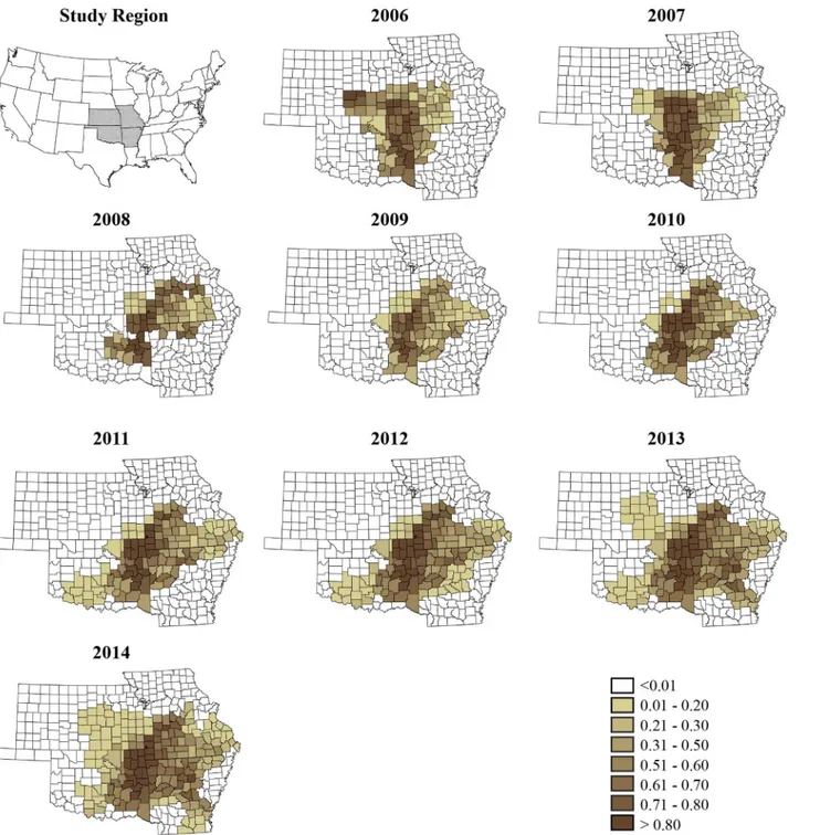
inFig 2, showing a clearly increasing trend for the region with a slight decrease in the later part of the study. Plots of annual crude rate estimates for RMSF prevalence for individual years over the study period is depicted inFig 3, whileFig 4illustrates maps of Bayes smoothed annual RMSF estimated relative risks for the study period after adjusting for the random terms and covariate effects. The estimates are based on the Bayesian geostatistical covariate model with socio–economic and climatic predictors and correspond to the median of the posterior predic-tive distribution. The counties of high risk were identified by mapping county–specific differ-ential trends (posterior median ofCij) with values greater than 0 (Fig 5) after accounting for Table 6. Model fit and comparison criteria.
Model D pD DIC LS
Partial spatio–temporal model
Model–1: Non–parametric terms (γj,ψij) 4654.21 358.31 5012.52 0.31, 0.57
Model–2: Parametric terms (βj,ψij) 4012.34 302.11 4314.45 0.28, 0.51
Covariate model
Model–3:Model–2 +β1,. . .,β5. 4723.59 402.61 5126.20 0.32, 0.59
Model–4:Model–2 +β1,. . .,β4. 3951.27 247.64 4198.91 0.25, 0.48
Model–5:Model–2 +β1,. . .,β3. 3429.73 236.18 3665.91 0.21, 0.43
Dis the expected deviance,pDis the deviance derived from the expected values of parameters,DICis the deviance information criterion, andLSis the logarithmic score.
β1= poverty–status,β2= daytime LST,β3= relative humidity,β4= number of houses built in 2005 or before,β5= percent developed—medium intensity
area. The removal ofβ2, thenβ1one at a time resulted in modelDICvalues of 3984.24 and 3746.65, respectively, and were therefore retained in the Bayesian covariate model.
doi:10.1371/journal.pone.0150180.t006
Fig 2. The posterior median and 95% CrI for the overall time trend in the covariate model.
covariate effects in the final model. Higher values close to zero indicate counties with a high probability of difference from the overall trend.
4. Discussion
The smoothed risk maps of relative risk produced in this study show all areas in the region that are affected by RMSF year after year, and are superior to maps of crude rate estimates, largely Fig 3. County–level crude rate estimates of Rocky Mountain spotted fever prevalence reported to the state health departments for the study period, 2005–2014.
owing to the ability of Bayesian models to efficiently borrow information from neighboring areal units, and in tackling the low–number problem commonly associated with epidemiologi-cal data in some areal units versus others. A primary concern in this study however was to identify the presence of any overall trend for the region, and to isolate high risk counties where disease trend could be increasing. We therefore specified appropriate random effect terms in a Bayesian framework to identify an overall time trend, and any space–time interaction effect, Fig 4. County–specific Bayesian smoothed estimates (posterior median) of Rocky Mountain spotted fever prevalence for the study period between years 2005–2014.
followed by the addition of different covariates that would explain additional variability in the data due to space–time effect. Although a descriptive plot of the reported numbers of cases to the health departments (seeFig 1) show a declining trend for Missouri, and a more or less sta-ble trend for Kansas, this study has identified a steadily increasing overall time trend for RMSF for all four contiguous states combined during the study period, indicating that RMSF has in fact increased year by year in the overall region, which are not visible when simply the crude numbers are plotted. Maps of counties with positive differential trends (Cij>0) represent
Fig 5. Posterior median of county–specific differential trends. Counties with values closer to 0 indicate a higher risk for RMSF.
higher risk for RMSF compared to other counties in the region, and can be seen to have increased in area over the years and expanded outwards from a central focus in 2006 bordering all four states towards all the directions in subsequent years. These findings have implications for prevention and management strategies of RMSF.
The notable abrupt increase in the number of cases during the 2011–2012 period in Arkan-sas and Oklahoma could be attributed to a number of factors, including changes to reporting practices employed by the state health departments in their respective states that may have temporarily increased interest in case reporting, and as well as changes to diagnostic methods adopted by laboratories during this period, which may have improved the accuracy levels by which different tick–borne diseases are identified. It is evident through the state health depart-ments of Arkansas and Oklahoma that they made a strong push for improving submission rates for tick-borne disease cases through awareness and education campaigns during the 2010–2011 period. Also, increasingly more diagnostic laboratories in the region are adopting molecular methods based onin vitroamplification procedures for rapidly detecting multiple tick-borne diseases, reasons that could have played a role in the noticed surge. The presence of environmental or climatic linkages behind this surge is also conceivable, but they could not be adequately evaluated in the present study due to data limitations. However, such evaluation of any associations, particularly with climatic patterns is worthy of further consideration. The winter and spring months of the year 2012 was unusually warm and humid in the Midwestern U.S [42], [43]. Even though a prolonged low pressure system over the Midwest lead to a drought in the summer of 2012, conditions earlier in the tick season may have favored a higher population growth and the proliferation of pathogens.
Poverty status of individuals in the four states was a strong predictor of RMSF in this study. In an earlier study we identified poverty status to be a significant predictor of another tick-borne disease, human monocytic ehrlichiosis in the same region as well [28]. Such associations of tick-borne diseases with socio–economic conditions are rarely evaluated in North America; however, lower socio–economic conditions were stronger predictors of tick-borne encephalitis in Europe compared to climatic and environmental predictors [23], [44]. This recurring associ-ation is perhaps indicative of higher exposure to tick pathogens for low–income individuals, who may work outdoors, and lower literacy levels and less awareness towards preventing tick-borne illnesses could be contributing factors.
There is notable interest in understanding the implications of ongoing climate–change on incidences of vector–borne diseases worldwide [10], [14], [45]. Climatic conditions affect arthropod phenology, population dynamics and their distribution over space, and the recent changes noted in shifting spatial range of some tick vectors [46], extended activity period due to relatively warmer conditions during winter [47], and changes to questing behavior all have been suspected to be influenced by climate–change [48], [49]. Whilst a strong emphasis is placed on researching the effect of climate change on disease–spreading arthropod vectors, the detection and then ascribing climate–change to increased disease incidences is however prob-lematic since there are many confounding players involved in such systems. Even though ongo-ing climate change is conceivably an influential driver in vector–borne disease systems, its relative importance over social, economic and demographic factors is debated [23]. This study further shows that a mixture of factors are important in the spatio–temporal patterns or the eco-epidemiology of tick–borne diseases, including such factors as poverty status and they need to be accounted for in modeling climate–change implications on vector–borne diseases.
conditions are vital for tick survival and it is an important delimiter to their spatial distribution [51], and relative humidity can often be seen associated with the survival and abundance of ticks in the literature, with higher humidity conditions often favoring the long–term survival of some ticks species’life stages through dry seasons [48] among other reasons. The higher day-time land surface temperature identified in this study is likely an indication of the average tem-perature conditions in some counties that are unfavorable forDermacentorticks versus others. Potential temperature effects on ticks and tick–pathogen interactions have been noted [52], and studies aiming to understand any physiological effects onDermacentorticks andR. rickett-siiinteraction in their host are worthy of consideration.
Some limitations of the study need to be mentioned. Even thoughR.rickettsiiis identified as the causative agent for RMSF, multipleRickettsiaspecies are vectored by ticks—many known to infect humans, which lead to similar clinical symptoms to that of RMSF [53]. These other
Rickettsiaspp. also cross-react in diagnostic tests that are currently performed for confirming
RMSF status, leading to poor test specificity [54]. The extent to which cases were wrongly iden-tified as RMSF in the present dataset cannot be reliably verified, although a majority of the cases are likely to beR.rickettsiicausing RMSF. We expect that the use of PCR–based diagnos-tic methods versus the current serology–based diagnosis will alleviate the misdiagnosis in the future and a clearer picture of the space–time dynamics of RMSF will become evident.
5. Conclusions
Results of this study show that Rocky Mountain spotted fever incidence in the central Midwest-ern states of Kansas, Missouri, Oklahoma and Arkansas have increased over the past decade, with high risk counties for this disease lying in the central and southern portions of the region. At the scale of a county, the spatial and spatio-temporal covariates of poverty level and average relative humidity are positively influential for incidence levels, while average day time land sur-face temperatures above 35°C is a limiting factor. Future epidemiological studies on this disease and other tick-borne diseases will benefit by considering socio-economic status of individuals, particularly poverty status. The identification of climate–change indices as important drivers of RMSF in this study is significant in the context of climate–change impacts on infectious diseases.
Acknowledgments
The authors are grateful to the epidemiologists at the state health departments of Kansas, Mis-souri, Oklahoma and Arkansas for providing RMSF data used in this study, and Mal Hoover, and Gina Scott, College of Veterinary Medicine, Kansas State University for providing excellent technical assistance. This study was supported in part by the PHS grant number AI070908 from the National Institute of Allergy and Infectious Diseases, National Institutes of Health, USA. This article is a contribution (Contribution no. 16-222-J) from the Kansas Agricultural Experiment Station. Publication cost for this article was provided by the K-State Open Access Publishing (KOAPF) program.
Author Contributions
References
1. Burgdorfer W. A Review of Rocky Mountain Spotted Fever (Tick-borne Typhus), its agent, and its tick vectors in the United States. J Med Entomol. 1975; 12: 269–278. PMID:810584
2. Dantas–Torres F. Rocky Mountain Spotted Fever. Lancet Infect Dis. 2007; 7: 724–732. PMID:
17961858
3. Centers for Disease Control and Prevention. Rocky Mountain spotted fever (RMSF). Available:http:// www.cdc.gov/rmsf/.
4. Centers for Disease Control and Prevention. Rocky Mountain spotted fever (RMSF). Statistics and epi-demiology. Available:http://www.cdc.gov/rmsf/stats/.
5. Masters EJ, Olson GS, Weiner SJ, Paddock CD. Rocky Mountain spotted fever: A clinician's dilemma. Arch Intern Med. 2003; 163: 769–774. PMID:12695267
6. Chen LF, Sexton DJ. What's new in Rocky Mountain spotted fever? Infect Dis Clin North Am. 2008 Sep; 22(3):415–32, vii–viii. doi:10.1016/j.idc.2008.03.008PMID:18755382
7. Dahlgren FS, Holman RC, Paddock CD, Callinan LS, McQuiston JH. Fatal Rocky Mountain spotted fever in the United States, 1999–2007. Am J Trop Med Hyg. 2012 Apr; 86(4):713–9. doi:10.4269/
ajtmh.2012.11-0453PMID:22492159
8. Treadwell TA, Holman RC, Clarke MJ, Krebs JW, Paddock CD, Childs JE. Rocky Mountain spotted fever in the United States, 1993–1996. Am J Trop Med Hyg. 2000; 63: 21–26. PMID:11357990 9. Openshaw JJ, Swerdlow DL, Krebs JW, Holman RC, Mandel E, Harvey A, et al. Rocky Mountain
spot-ted fever in the Unispot-ted States, 2000–2007: Interpreting contemporary increases in incidence. Am J
Trop Med Hyg. 2010 Jul; 83(1):174–82. doi:10.4269/ajtmh.2010.09-0752PMID:20595498 10. Githeko AK, Lindsay SW, Confalonieri UE, Patz JA. Climate change and vector–borne diseases: A
regional analysis. Bulletin of the World Health Organization 2000; 78: 1136–1147. PMID:11019462 11. Altizer S, Ostfeld RS, Johnson PT, Kutz S, Harvell CD. Climate change and infectious diseases: From
evidence to a predictive framework. Science. 2013 Aug 2; 341(6145):514–519. doi:10.1126/science.
1239401PMID:23908230
12. Thomson MC. Emerging infectious diseases, vector–borne diseases, and climate change. In:
Freed-man B, editor. Global Environmental Change. Netherlands: Springer; 2014. pp. 623–628.
13. Randolph SE, Rogers DJ. Fragile transmission cycles of tick-borne encephalitis virus may be disrupted by predicted climate change. Proc. R. Soc. Lond. B. doi:10.1098/rspb.2000.1204
14. Ogden NH, Mechai S, Margos G. Changing geographic ranges of ticks and tick-borne pathogens: driv-ers, mechanisms and consequences for pathogen diversity. Front Cell Infect Microbiol. 2013 Aug 29; 3:46. doi:10.3389/fcimb.2013.00046eCollection 2013. PMID:24010124
15. Ostfeld RS, Brunner JL. Climate change and Ixodes tick-borne diseases of humans. Philos Trans R Soc Lond B Biol Sci. 2015 Apr 5; 370(1665). pii: 20140051. doi:10.1098/rstb.2014.0051PMID: 25688022
16. Bakken JS, Folk SM, Paddock CD, Bloch KC, Krusell A, Sexton DJ, et al. Diagnosis and management of tickborne rickettsial diseases: Rocky Mountain spotted fever, ehrlichioses, and anaplasmosis–United
States. A practical guide for physicians and other health care and public health professionals. MMWR Recomm Rep. 2006; 55:1–27.
17. Kovats RS, Campbell–Lendrum DH, McMichel AJ, Woodward A, Cox JSH. Early effects of climate
change: Do they include changes in vector–borne disease? Philos T R Soc B. 2001; 356: 1057–1068. 18. McCarty JP. Ecological consequences of recent climate change. Conserv Biol, 2001; 15: 320–331. 19. Moncayo AC, Cohen SB, Fritzen CM, Huang E, Yabsley MJ, Freye JD et al. Absence ofRickettsia
rick-ettsiiand occurrence of other spotted fever group rickettsiae in ticks from Tennessee. The American
journal of tropical medicine and hygiene, 2010; 83: 653–657. doi:10.4269/ajtmh.2010.09-0197PMID:
20810834
20. Stromdahl EY, Jiang J, Vince M, Richards AL. Infrequency ofRickettsia rickettsiiinDermacentor
varia-bilisremoved from humans, with comments on the role of other human-biting ticks associated with
spot-ted fever group rickettsiae in the Unispot-ted States. Vector-borne and Zoonotic Diseases 2011; 11: 969–
977. doi:10.1089/vbz.2010.0099PMID:21142953
21. Demma LJ, Traeger MS, Nicholson WL, Paddock CD, Blau DM, Eremeeva ME, et al. Rocky Mountain spotted fever from an unexpected tick vector in Arizona. New Engl J Med. 2005; 353: 587–594. PMID:
16093467
22. Patz JA, Campbell–Lendrum D, Holloway T, Foley JA. Impact of regional climate change on human
health. Nature 2005; 438: 310–317. PMID:16292302
24. Gray JS, Dautel H, Estrada–Peña A, Kahl O, Lindgren E. Effects of climate change on ticks and
tick-borne diseases in Europe. Interdiscip Perspect Infect Dis. 2009; 2009:593232. doi:10.1155/2009/ 593232Epub 2009 Jan 4. PMID:19277106
25. Knorr–Held L. Bayesian modelling of inseparable space–time variation in disease risk. Stat Med. 1999;
19: 2555–2567
26. Lawson AB. Bayesian disease mapping: hierarchical modeling in spatial epidemiology. 1 st. ed. Boca Raton: CRC press; 2013.
27. Kang SY, McGree J, Mengersen K. Bayesian hierarchical models for analysing spatial point–based
data at a grid level: A comparison of approaches. Environ Ecol Stat. 2014; 22: 297–327.
28. Raghavan RK, Neises D, Goodin DG, Andresen DA, Ganta RR. Bayesian spatio–temporal analysis
and geospatial risk factors of human monocytic ehrlichiosis. PLoS One. 2014 Jul 3; 9(7):e100850. doi: 10.1371/journal.pone.0100850eCollection 2014. PMID:24992684
29. Fry J, Xian G, Jin S, Dewitz J, Homer C, Yang L, et al. Completion of the 2006 National Land Cover Database for the Conterminous United States, PE&RS, 2011; 77: 858–864.
30. Land Processes Distributed Active Archive Center. MODIS overview. Available:https://lpdaac.usgs. gov/products/modis_products_table/modis_overview.
31. White J, Hoogenboom G, Stackhouse P, Hoell J. Evaluation of NASA satellite and assimilation model–
derived long–term daily temperature data over the continental US. Agr Forest Meteorol. 2008; 148:
1574–1584.
32. Minnesota Population Center. National Historical Geographic Information System: Version 2.0. Minne-apolis, MN: University of Minnesota 2011. Available:http://www.nhgis.org.
33. Hosmer DW Jr., Lemeshow S, Sturdivant RX. Model-Building Strategies and Methods for Logistic Regression In: Hosmer DW Jr., Lemeshow S, Sturdivant RX, editors. Applied Logistic Regression, Third Edition, Hoboken: John Wiley & Sons Inc.; 2013. pp. 89–151.
34. Rue H, Held L. Gaussian Markov random fields: Theory and applications. Boca Raton: Chapman & Hall/CRC; 2005.
35. Schrödle B, Held L. Spatio-temporal disease mapping using INLA Environmetrics 2011; 22: 725–734. 36. Bernardinelli LD, Clayton C, Pascutto C, Montomoli M, Ghislandi M Songini M Bayesian analysis of
space–time variation in disease risk. Stat Med. 1995; 14: 2433–2443. PMID:8711279
37. Spiegelhalter DJ, Best NG, Carlin BP, Van Der Linde A Bayesian measures of model complexity and fit. J R Stat Soc B Met. 2002; 64: 583–639.
38. Plummer M Penalized loss functions for Bayesian model comparison. Biostatistics 2008; 9: 523–539.
doi:10.1093/biostatistics/kxm049PMID:18209015
39. Gneiting T, Raftery AE. Strictly proper scoring rules, prediction, and estimation. J Amer Statist Assoc. 2007; 102: 359–378.
40. Rue H, Martino S, Chopin N. Approximate Bayesian inference for latent Gaussian models by using Inte-grated Nested Laplace Approximations. J R Stat Soc B Met. 2009; 71: 319–392.
41. R–INLA Random walk model of order 1. Available:http://www.math.ntnu.no/inla/r-inla.org/doc/latent/
rw1.pdf.
42. NOAA National Climatic Data Center. BAMS state of the climate 2012. Available:http://www.ncdc. noaa.gov/bams-state-of-the-climate/2012.php.
43. Hoerling M, Eischeid J, Kumar A, Leung R, Mariotti A, Mo K, et al. Causes and predictability of the 2012 Great Plains drought. Bull. Am. Meteorol. Soc. 2014; 95: 269–282. doi:10.1175/bams-d-13-00055.1 44. Stefanoff P, Rosinska M, Samuels S, White DJ, Morse DL, Randolph SE A National case–control study
identifies human socio–economic status and activities as risk factors for tick-borne encephalitis in
Poland. PLoS One. 2012; 7(9):e45511. doi:10.1371/journal.pone.0045511Epub 2012 Sep 19. PMID: 23029063
45. Randolph SE. Is Expert Opinion Enough? A critical assessment of the evidence for potential impacts of climate change on tick-borne diseases. Anim Health Res Rev. 2013 Dec; 14(2):133–7. doi:10.1017/
S1466252313000091Epub 2013 Sep 26. PMID:24067445
46. Porretta D, Mastrantonio V, Amendolia S, Gaiarsa S, Epis S, Genchi C, et al. Effects of global changes on the climatic niche of the tick Ixodes ricinus inferred by species distribution modelling. Parasit Vec-tors. 2013 Sep 19; 6:271. doi:10.1186/1756-3305-6-271PMID:24330500
47. Estrada–Peña A, Martinez JM, Sanchez Acedo C, Quilez J, Del Cacho E. Phenology of the tick, Ixodes
ricinus, in its southern distribution range (central Spain). Med Vet Entomol. 2004; 18: 387–397. PMID:
48. Medlock JM, Hansford KM, Bormane A, Derdakova M, Estrada–Peña A, George JC, et al. Driving
forces for changes in geographical distribution ofIxodes ricinusticks in Europe. Parasit Vectors. 2013 Jan 2; 6:1. doi:10.1186/1756-3305-6-1PMID:23281838
49. United States Environmental Protection Agency. Climate change indicators in the united states, 2014. 3 rd. ed. Available:http://www3.epa.gov/climatechange/pdfs/climateindicators-full-2014.pdf.
50. Knulle W, Rudolph D. Humidity relationships and water balance of ticks. In: Obenchain FD, Galun R, editors. Physiology of Ticks, 1982. pp. 43–70.
51. Raghavan RK, Goodin DG, Hanzlicek GA, Zolnerowich G, Dryden MW, Anderson GA, et al. Maximum entropy–based ecological niche model and bio–climatic determinants of lone star tick (Amblyomma
americanum) niche. Vector-Borne Zoonot. doi:10.1089/vbz.2015.1837Epub 2016 Jan 29.
52. Estrada–Peña A, Ayllón N, De La Fuente J. Impact of climate trends on tick-borne pathogen
transmis-sion. Front Physiol. 2012 Mar 27; 3:64. doi:10.3389/fphys.2012.00064eCollection 2012. PMID: 22470348
53. Centers for Disease Control and Prevention. Other Tick-borne Spotted Fever Rickttsial Infections. http://www.cdc.gov/otherspottedfever/.