www.earth-syst-dynam.net/7/535/2016/ doi:10.5194/esd-7-535-2016
© Author(s) 2016. CC Attribution 3.0 License.
Radiative forcing and feedback by forests in warm
climates – a sensitivity study
Ulrike Port1, Martin Claussen1,2, and Victor Brovkin1
1Max Planck Institute for Meteorology, 20146 Hamburg, Germany 2Meteorological Institute, University of Hamburg, 20146 Hamburg, Germany
Correspondence to:Ulrike Port ([email protected])
Received: 20 November 2015 – Published in Earth Syst. Dynam. Discuss.: 14 December 2015 Revised: 23 April 2016 – Accepted: 22 May 2016 – Published: 6 July 2016
Abstract. We evaluate the radiative forcing of forests and the feedbacks triggered by forests in a warm, basically ice-free climate and in a cool climate with permanent high-latitude ice cover using the Max Planck Institute for Meteorology Earth System Model. As a paradigm for a warm climate, we choose the early Eocene, some 54 to 52 million years ago, and for the cool climate, the pre-industrial climate, respectively. To isolate first-order effects, we compare idealised simulations in which all continents are covered either by dense forests or by deserts with either bright or dark soil. In comparison with desert continents covered by bright soil, forested continents warm the planet for the early Eocene climate and for pre-industrial conditions. The warming can be attributed to different feedback processes, though. The lapse-rate and water-vapour feedback is stronger for the early Eocene climate than for the pre-industrial climate, but strong and negative cloud-related feedbacks nearly outweigh the positive lapse-rate and water-vapour feedback for the early Eocene climate. Subsequently, global mean warming by forests is weaker for the early Eocene climate than for pre-industrial conditions. Sea-ice related feedbacks are weak for the almost ice-free climate of the early Eocene, thereby leading to a weaker high-latitude warming by forests than for pre-industrial conditions. When the land is covered with dark soils, and hence, albedo differences between forests and soil are small, forests cool the early Eocene climate more than the pre-industrial climate because the lapse-rate and water-vapour feedbacks are stronger for the early Eocene climate. Cloud-related feedbacks are equally strong in both climates. We conclude that radiative forcing by forests varies little with the climate state, while most subsequent feedbacks depend on the climate state.
1 Introduction
In present-day climate, forests tend to warm the high lati-tudes by masking the bright snow cover leading to a lower surface albedo than with bare soil or grass (Bonan, 1992; Betts and Ball, 1997; Bonan, 2008), and this warming can be amplified by the sea-ice albedo feedback (Claussen et al., 2001; Fraedrich et al., 2005; Brovkin et al., 2009). In the tropics, forests tend to cool the climate by enhancing tran-spiration and evaporation which leads to an increased cloud cover and a higher planetary albedo. The enhanced transpi-ration and evapotranspi-ration by trees increase the latent heat flux resulting in further cooling (Bathiany et al., 2010). In our study, we explore the question whether these
biogeophysi-cal effects of forests remain the same amplitude in a much warmer, ice-free climate. Instead of prescribing an artificially ice-free pre-industrial climate, we choose a palaeo-climate set-up.
and ice cover appears to be strong in the studies by Otto-Bliesner and Upchurch (1997) and Liakka et al. (2014), be-cause substantial snow and sea-ice coverage occurs in win-ter and spring in their simulations. In a climate that was presumably warmer than the late Cretaceous or the Eocene Oligocene Transition and nearly free of ice, the snow mask-ing effect and the ice albedo feedback would vanish leadmask-ing to a considerably different biogeophysical effect by vegeta-tion than in the present-day climate. Alkama et al. (2012) analyse the impact of global desertification in present-day climate, in the cold climate of the last glacial maximum, and in a warm climate caused by an increase in greenhouse gas concentrations. They find that the reduction of upward la-tent heat fluxes dominates the prevailing signal in terms of surface energy budget. In their simulations, desertification yields a similar temperature response for all climate states in regions south of 20◦N. At high latitudes, the effect of
de-sertification differs because of the difference in snow albedo feedback.
Here, we choose the early Eocene climate (54–52 Ma) which was a warm, presumably nearly ice-free climate. Trop-ical temperatures were 5 to 6 K higher than today (Pearson et al., 2007), and polar temperatures were above the freez-ing point durfreez-ing most time of the year leadfreez-ing to almost ice-free poles (Hutchison, 1982; Markwick, 1994; Ivany et al., 2006; Zachos et al., 1992). In agreement with proxy data (Za-chos et al., 1992), no permanent sea ice occurs for the early Eocene climate simulations by Heinemann et al. (2009).
In their modelling studies, Sewall et al. (2000) and Lopt-son et al. (2014) assess the sensitivity of the early Eocene climate to vegetation. Sewall et al. (2000) find that vegeta-tion cools regional climate in coastal Australia, central South America, central North America, and in south-central Africa. They trace the cooling back to an enhanced latent heat flux by vegetation leading to an increased cloud cover. The dynamic vegetation used by Loptson et al. (2014) warms the global mean Eocene climate relative to a homogeneous shrub cover by reducing surface albedo and enhancing humidity leading to a stronger greenhouse effect. Both studies consider the early Eocene climate only, while the studies mentioned at the beginning focus on the biogeophysical effect of vege-tation in present-day climate. Hence, a consistent quantita-tive comparison of the biogeophysical effect of vegetation in the warm, nearly ice-free and snow-free climate of the early Eocene and in the pre-industrial interglacial climate is not possible. To close this gap, we compare the biogeophysical effect of vegetation in both these climates using a consistent experimental set-up for both climates.
To disentangle direct biogeophysical effects and triggered feedbacks, we use the linear regression approach proposed by Gregory et al. (2004). This approach yields an estimate of the radiative forcing by forests and of the subsequent climate feedbacks. We expect that radiative forcing by forests de-pends on the soil albedo. To isolate the impact of soil albedo on the radiative forcing by forests, we specify different soil
albedo. First, we choose a value of 0.1 for soil albedo which is about the albedo of volcanic rocks and granite bedrock (Warner, 2004). In this case, soil and vegetation have sim-ilarly low values of albedo. Second, we assume a homoge-neous soil albedo of 0.4, i.e. a value representative for bright soil, which has a much higher albedo than the forests have.
For the early Eocene climate and the pre-industrial cli-mate, we prescribe an atmospheric CO2 concentration of
560 and 280 ppm, respectively. In other words, we neglect the CO2uptake by forests and focus on the biogeophysical
effect of forests.
2 Model and experiments
2.1 MPI-ESM
The MPI-ESM consists of the atmospheric general circula-tion model ECHAM6 (Stevens et al., 2013), the Max Planck Institute Ocean Model (MPIOM) (Jungclaus et al., 2013), the land surface scheme JSBACH (Reick et al., 2013), and the ocean biogeochemistry model HAMOCC (Ilyina et al., 2013). ECHAM6 and JSBACH run in a horizontal resolution of T31, which corresponds to approximately 3.75◦×3.75◦.
ECHAM6 considers 31 levels in the vertical up to 10 hPa. The ocean grid has a resolution of about 3◦and consists of
40 levels in depth.
The JSBACH model simulates fluxes of energy, water, mo-mentum, and CO2 between the land surface and the
atmo-sphere (Raddatz et al., 2007). To represent vegetation compo-sition, land grid cells in JSBACH are divided into tiles (frac-tions). Those tiles are covered with several plant functional types or PFTs (trees, shrubs, and grasses), and two types of bare surface and seasonally bare soil and permanently bare ground, or desert (Brovkin et al., 2009; Reick et al., 2013). In the JSBACH model setup used in this study, the fraction of land surface covered with particular PFTs is prescribed and phenology (LAI) is kept constant throughout the season in order to simplify the analysis of interactions between land and atmosphere.
2.2 Early Eocene set-up
Table 1.Boundary conditions for the early Eocene climate simula-tions and for pre-industrial condisimula-tions simulasimula-tions.
Pre-industrial Early Eocene CO2concentration 280 ppm 560 ppm
Methane 0.8 ppm 0.8 ppm
Nitrous oxide 0.288 ppm 0.288 ppm Orbit pre-industrial pre-industrial
Bathymetry and orography present-day Bice and Marotzke (2001) Ice sheets pre-industrial none
north pole of the ocean grid to Palaeo-Asia and the grid south pole to Palaeo-South America.
Following Heinemann et al. (2009), the atmospheric CO2
concentration is fixed to 560 ppm (Table 1), which repre-sents the lower limit of reconstructions (Zachos et al., 2001; Beerling and Royer, 2011). Estimates of other greenhouse gases, like methane and nitrous oxide, are absent for the early Eocene. Thus, we proceed as Heinemann et al. (2009) and prescribe pre-industrial values for methane and nitrous oxide for the early Eocene atmosphere (Table 1). We decide to use a pre-industrial orbit in our early Eocene simulations. This ap-proach limits the differences between the early Eocene and the pre-industrial boundary conditions to the distribution of continents, the bathymetry, the appearance of ice sheets, and the atmospheric CO2concentration (Table 1).
To achieve an initial equilibrium climate, we simulate the Eocene climate starting from the equilibrium climate by Heinemann et al. (2009). Like in their simulation, we assume a globally homogeneous savanna vegetation with a desert cover of 40 %, a tree cover of 24 %, and a grass cover of 36 %. After 300 years, near-surface temperature and upper-level ocean temperatures are in equilibrium. Only in the deep ocean, a marginal temperature trend of some 0.04 K per 100 years remains.
To evaluate the equilibrium Eocene climate, which we use as initial state for all Eocene simulations, we compare the simulated climate against the marine and terrestrial temper-ature reconstructions used by Lunt et al. (2012) and Huber and Caballero (2011), respectively. Lunt et al. (2012) merge palaeotemperature estimates at the sea surface, near the sea surface, and in shallow inner-shelf bottom water based on oxygen isotope (δ18O) values, on Magnesium–Calcium ra-tios (Mg/Ca) derived from planktic foraminifera, and on TEX86. In all measurement sites, several methods have been
applied to estimate temperature. Like Lunt et al. (2012), we use the average over all temperature estimates in one site. The compilation includes temperature reconstructions from just before the onset of the Paleocene-Eocene thermal maxi-mum (PETM) (∼55 Ma) until the Early Eocene climatic op-timum (EECO) (∼50–52 Ma). Temperature estimates of the PETM itself and of the EECO are excluded in our compari-son to the simulated Eocene climate.
1
2
Figure 1.Annual mean 2 m temperature for the early Eocene simu-lation in shaded colours. Stars show reconstructed annual mean sea surface temperature (SST) and near-surface temperature of the early Eocene derived fromδ18O, Mg/Ca, and TEX86(Lunt et al., 2012). Numbers 1 and 2 mark SST reconstructions by Sluijs et al. (2006) and Bijl (2009), respectively. Circles refer to terrestrial annual mean temperature estimates based on macrofloral and palynoflora assem-blage data and from teeth, hydrogen isotopes, and oxygen isotopes (Huber and Caballero, 2011).
Huber and Caballero (2011) provide a compilation of annual mean temperature for the early Eocene based on terrestrial proxy data. Most temperature estimates in this compilation result from the analysis of macrofloral assem-blage data using the Climate Leaf Analysis Multivariate Pro-gram (CLAMP) (Wolfe, 1995) and the leaf margin analysis (LMA; Wilf, 1997). Further, the data base includes temper-ature estimates based on teeth, hydrogen isotopes, oxygen isotopes, and palynoflora assemblage data.
The simulated annual mean temperatures show a good agreement with the temperature estimates in the tropics and subtropics (Fig. 1), while discrepancies appear in the mid- to high latitudes. In the mountainous terrain in North America, the temperature estimates vary over small distances because the altitude does. Our model fails to resolve the small-scale orography leading to a mismatch of simulated and recon-structed temperature.
In the northern high latitudes, terrestrial temperature re-constructions are 5 to 11 K higher than the simulated tem-perature. Especially, the marine temperature reconstruction by Sluijs et al. (2006) strongly exceeds the simulated annual mean temperature north of Greenland (Fig. 1). This SST es-timate is based on TEX86, which likely has a bias to
repre-sent summer temperatures (Sluijs et al., 2006). Considering summer temperatures, our model produces a 5 K lower tem-perature than suggested by Sluijs et al. (2006).
In the southern high latitudes, the simulation agrees with marine and terrestrial temperature estimates. The only excep-tion is the SST reconstrucexcep-tion by Bijl (2009) that suggests a temperature of 24◦C at the Tasman Plateau (Fig. 1). Like the estimate by Sluijs et al. (2006), the estimate by Bijl (2009) is based on TEX86 and likely has a bias to summer
Table 2.Simulations performed with boundary conditions for the early Eocene climate and the pre-industrial climate. The listed veg-etation cover is prescribed on all ice-free continents. The values for the land surface albedo refer to snow-free regions. In the desert world, the surface albedo equals the soil albedo. In the forest world, trees cover the soil completely and the albedo of the forests deter-mines land surface albedo.
Vegetation Land surface albedo
Dark desert world none 0.1 Bright desert world none 0.4 Forest world 100 % tree cover 0.12
The cold bias in the high latitudes is a common prob-lem when simulating the early Eocene climate as Lunt et al. (2012) show within the Eocene Modelling Intercomparison Projects (EoMIP). In comparison to the models participating in the EoMIP, our model is within the range of other model results indicating that our background climate represents the early Eocene climate about as well as simulations from other state-of-the-art models do. Further, we seek to investigate the biogeophysical effect of vegetation in a warm, nearly ice-free background climate instead of to simulate the early Eocene as realistically as possible. Since sea ice occurs only in a few years in our simulation and snow appears only during polar night in central Antarctica and in the High North, this Eocene simulation is suitable for our purpose.
2.3 Simulations
Starting from our early Eocene background climate, we per-form three simulations (Table 2). In thedark desert world, we replace the savanna vegetation by deserts with a soil albedo of 0.1. Similarly, no vegetation exists in the bright desert world, but this time, soil albedo is 0.4. In the forest world, all continents are completely covered with forests. The vege-tation cover is static and the leaf area index (LAI) is constant throughout the whole simulation independent of season, tem-perature, and water availability. We distinguish between trop-ical and extra-troptrop-ical trees (Fig. 2). The boundary between tropical trees and extra-tropical trees is prescribed based on the climatic limits of tropical trees computed from off-line simulations by Heinemann et al. (2009) for the Eocene cli-mate and by Port et al. (2012) for the pre-industrial clicli-mate. Tropical trees have a LAI of 7 and a roughness length of 2 m. Extra-tropical trees have a LAI of 5 and a roughness length of 1 m. To facilitate comparison between the Eocene and the pre-industrial simulations, we ignore that the climatic requirements for tropical trees differ between the Eocene and the pre-industrial case. (This will be re-assessed in the last section.) The soil albedo does not matter in the forest world. This was tested by simulating the forest world climate with
Figure 2.Vegetation cover in the forest world for the pre-industrial climate(a)and the early Eocene climate(b). Extra-tropical trees and tropical trees differ concerning their LAI and roughness length.
low and high soil albedo, respectively. Both soil albedo val-ues yield the same climate (not shown) because trees com-pletely mask the soil leading to a land surface albedo of ap-proximately 0.12 in snow-free regions in the forest world.
Consistent with the Eocene simulations, we perform three simulations with industrial boundary conditions. All pre-industrial simulations start from the equilibrium climate by Port et al. (2012), whose pre-industrial simulation ran for 1000 years, with dynamic vegetation cover and an atmo-spheric CO2concentration of about 280 ppm. In the first time
step, we replace the mixed pre-industrial vegetation cover with dark desert, bright desert, and forests in the dark desert world, bright desert world, and forest world simulation, re-spectively. Ice sheets on Greenland and Antarctica remain unchanged.
3 Methods
The simulations – dark desert world, bright desert world, for-est world – last for 400 years. After that period, climate has approached, but not yet reached, an equilibrium at the end of the simulations. To estimate the impact of forests on cli-mate from these (still unequilibrated) simulations, we quan-tify the radiative forcing by forests and the subsequent cli-mate feedbacks by using the linear regression approach by Gregory et al. (2004). This method has proven to be very useful to analyse radiative forcing and feedback triggered by a strong, large-scale perturbation from transient simulations. The advantage of this method is that the first decades after the perturbation are sufficient to estimate radiative forcing and feedbacks, and climate does not need to be simulated until the new equilibrium is reached.
relates approximately linearly to the changes in surface tem-perature,1T,
1R(t)=1Q+λ1T(t). (1)
The instantaneous response of the TOA radiation balance to the modification of the land surface is the radiative forc-ing,1Q. The climate feedback parameter,λ, quantifies the strength of feedbacks between1T and1R.
From the model simulations, we calculate global annual mean values for1R and1T, and obtain pairs of1Ri and
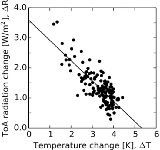
1Ti for each year, i. Figure 3 shows the points of (1Ti,
1Ri) for the early Eocene dark desert world simulation. In the initial equilibrium climate, savanna covers all continents but in the first year of the dark desert simulation, we replace savanna by dark bare soil. During the simulation, the sim-ulated climate progressively approaches a new equilibrium. The straight line fitted to the points of (1Ti,1Ri) reveals the parameters in Eq. (1) (Gregory et al., 2004). At the in-tersection of the regression line with the 1R axis, 1R is the radiative forcing 1Q. The slope of the regression line is the feedback parameter λ. Here, the regression line has a negative slope,λ, indicating that feedbacks counteract the perturbation in the TOA radiation balance. In other words, feedbacks stabilise climate.
The linear regression further allows one to estimate the equilibrium temperature change by deforestation. At the in-tersection of the regression line with the 1T-axis, the per-turbation in TOA radiative flux becomes zero and the tem-perature is in a new equilibrium. The according estimated equilibrium temperature change is
1Teq= −1Q
λ . (2)
Li et al. (2012) assess the question whether the Gregory method reveals a realistic estimate for the equilibrium near-surface warming in response to a doubling of atmospheric CO2 concentration. They find that the Gregory method
un-derestimates equilibrium warming by only 10 % relative to a simulation which runs until equilibrium is reached. Their results let us assume that the Gregory method provides a rea-sonable estimate of the equilibrium temperature change.
The feedback parameter is evaluated from the slope of the regression line which could change with time. For the first decades after a perturbation, however, Gregory et al. (2004) find a constant slope. In line with Andrews et al. (2012), we hence consider the first 150 years of our simulation for the regression.
For the forest world simulation, the linear regression ap-proach reveals the radiative forcing and the feedbacks by af-foresting savanna-like vegetation. However, we aim to esti-mate the radiative forcing and the feedbacks from afforest-ing deserts on all continents. Hence, we modify the linear regression approach in the way that we combine the forest world simulation with the desert world simulations. Let1Rd
0 1 2 3 4 5 6
Temperature change [K],
∆T
0.0
1.0
2.0
3.0
4.0
To
A r
ad
iat
ion
ch
an
ge
[W
/m
2
],
∆
R
Figure 3.Evolution of radiative flux at the top of the atmosphere with temperature changes at the surface in the dark desert world of the early Eocene climate. At the beginning of the simulation, savanna-like vegetation is replaced by bare soil with an albedo of 0.1. The first 150 simulated years are shown. The black line is the fitted regression line.
be the perturbation of the net TOA radiation in the case of replacing savanna with desert, and let1Rfbe the
perturba-tion in the case of replacing savanna with forest. In the linear approach, the difference,1Rfd, is the perturbation due to
re-placing deserts by a complete forest cover. For each year in our simulation,i, we define
1Rfdi =1Rfi−1Rid. (3)
Consistently, we subtract the temperature differences of the two perturbation experiments to obtain
1Tfdi =1Tfi−1Tdi=Tfi−Tdi. (4)
Considering Eq. (1), the regression line to the points (1Tfdi,
1Rfdi ) is
1Rfd=1Qfd+λfd1Tfd. (5)
The radiative forcing of afforesting the desert world is ex-pressed by1Qfd. The according feedback parameter isλfd.
The equilibrium temperature response, 1Tfdeq, is approxi-mated by
1Tfdeq= −1Qfd λfd
. (6)
3.2 Decomposition of the radiation balance
The net perturbation in the TOA radiation balance consists of a long-wave component (LW) and a short-wave compo-nent (SW). Both compocompo-nents consist of a cloud share (cl) and a clear-sky share (cs) leading to
The clear-sky share in radiation represents the radiation when clouds are neglected. The cloud share refers to the difference between the clear-sky radiation and the all-sky radiation. We apply the linear regression technique on each of the four ra-diation components. The corresponding regression lines are described by
1RLWcl=1QLWcl+λLWcl1T , (8)
1RLWcs=1QLWcs+λLWcs1T , (9)
1RSWcl=1QSWcl+λSWcl1T , (10)
1RSWcs=1QSWcs+λSWcs1T . (11)
This approach separates net radiative forcing and feedback into the single components of radiation (Andrews et al., 2012).
The long-wave clear-sky feedback parameter, λLWcs,
quantifies mainly the sum of the Planck feedback, the water-vapour feedback, and the lapse-rate feedback. The Planck feedback refers to the modified emission of long-wave radia-tion when surface and troposphere change their temperature while keeping the vertical temperature gradient. For instance, a warming increases the emission of long-wave radiation by the surface leading to an energy loss at the top of the atmo-sphere. The energy loss counteracts the initial warming and stabilises the climate.
We estimate the Planck feedback parameter,λP, as
λP=
∂R
∂T = −4σ ǫT
3.
(12)
The term on the right-hand side consists of the Stefan-Boltzmann constant,σ, the global mean surface temperature in Kelvin [K],T, and the emissivity of the atmosphere,ǫ. The emissivity describes the strength of the greenhouse effect and varies depending on the climate state. We estimate ǫ from the ratio of long-wave radiation escaping at the top of the at-mosphere to long-wave radiation emitted by the surface. At the beginning of the simulations, ǫ is 0.585 and 0.541 for pre-industrial conditions and for the early Eocene climate, respectively, which reflects a stronger greenhouse effect in the warmer early Eocene climate. The corresponding global mean surface temperatures are 287 and 297 K, respectively. Considering these values, Eq. (12) reveals aλPof−3.1 and
−3.3 W m−2K−1 for pre-industrial conditions and for the early Eocene climate, respectively. Assuming that feedbacks act linearly, we subtractλPfromλLWcl. The remaining
feed-back parameter is mainly the lapse-rate and water-vapour feedback which we nameλWV+LR.
We quantify the uncertainty of radiative forcings and cli-mate feedbacks in terms of the 95 % confidence interval which we assess using bootstrapping. We randomly select 150 pairs of differences in temperature and TOA radiative flux out of the first 150 years of our simulation. Each pair of our simulation can be selected several times. We re-peat the resampling 10 000 times. From each time, we
es-0 1 2 3 4 5 6 7
Temperature difference [K],
∆T
1
3
5
7
To
A r
ad
iat
ion
di
ffe
ren
ce
[W
/m
2
],
∆
R
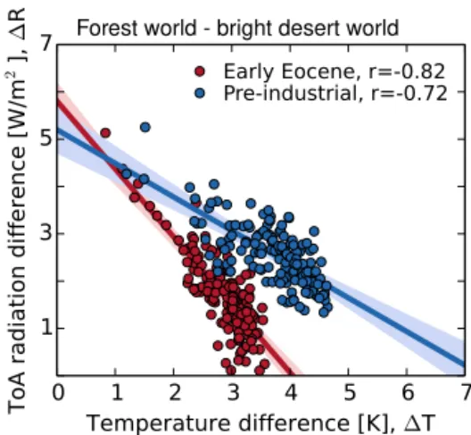
Forest world - bright desert worldEarly Eocene, r=-0.82
Pre-industrial, r=-0.72
Figure 4.Evolution of differences in the TOA radiative flux be-tween the forest world and the bright desert world with corre-sponding differences in near-surface temperature. Global annual-mean values are considered. Red and blue points relate to the early Eocene climate and to the pre-industrial climate, respectively. The first 150 years are shown and considered for the regression and the correlation coefficient,r. The shaded areas refer to the 95 % confi-dence interval for the regression lines.
timate the feedbacks and forcings. Then, we sort the result-ing 10 000 values. Truncatresult-ing the upper and lower 2.5 % pro-vides the 95 % confidence interval.
4 Results and discussion
4.1 Forestation of a bright desert world
Relative to the bright desert world, the forest world is 4.2 and 5.7 K warmer at the end of the early Eocene simulations and at the end of the pre-industrial simulations, respectively (Ta-ble 3). The warming results from a positive radiative forcing by trees which is 5.8 and 5.2 W m−2for the early Eocene cli-mate and for the pre-industrial clicli-mate. The forcings do not differ significantly at the 95 % level as the confidence interval in Fig. 4 illustrates.
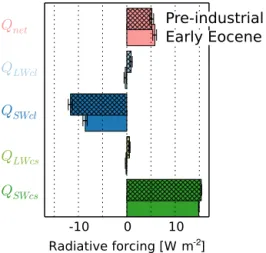
The largest component in net radiative forcing is the short-wave clear-sky radiative forcing,1QSWcs, which amounts to
some 15 W m−2 in both climate states (Fig. 5). The major mechanism leading toQSWcsis the surface albedo reduction
-10
0
10
Radiative forcing [W m ]
-2Pre-industrial
Early Eocene
QnetQLWcl
QSWcl
QLWcs
QSWcs
Figure 5.Net radiative forcing and its single components for the comparison of the forest world to the bright desert world. Hatched and plain bars show the radiative forcings for the pre-industrial cli-mate and the early Eocene clicli-mate, respectively. The error bars refer to the 95 % confidence interval.
albedo changes in both climate states are consistent with large values of1QSWcs.
The second pronounced component in radiative forcing is the short-wave cloud radiative effect, 1QSWcl, which
amounts to−8.6 and−11.6 W m−2for the early Eocene cli-mate and for the pre-industrial clicli-mate, respectively (Fig. 5).
1QSWcl describes the radiative impact of changes in cloud
cover as well as an indirect impact of clouds which we de-fine below as “masking effect”. In our simulations, cloud adjustment mainly refers to an increased cloud cover due to forests leading to a higher planetary albedo and a neg-ative radineg-ative forcing. This effect is especially strong over land, where forests strongly reduce surface albedo and the increased cloud cover compensates the surface albedo reduc-tion. Figure 6 illustrates the compensation of surface albedo reduction. Shown are the difference in planetary albedo and in cloud cover between the first year of the forest world sim-ulation and the first year of the desert world simsim-ulation. In general, planetary albedo over land decreases due to forests, but in the tropics, cloud cover increases which compensates the decrease in planetary albedo.
Beside cloud adjustment, 1QSWcl includes the cloud
masking effect. This effect is an artefact which results from separating full-sky radiation into the clear-sky component and the cloud component. If a dense cloud cover occurs in the forest world and in the desert world, full-sky short-wave radiative forcing will be weak. Clear-sky radiation, however, will be strongly positive due to the lower surface albedo in the forest world than in the desert world. Deriving the cloud forcing from the weak full-sky radiative forcing and the strongly positive clear-sky radiation reveals a strongly negative cloud radiative forcing even though cloud cover did not change. As1QSWclincludes cloud adjustment and cloud
masking, we can not disentangle both effects, and we can not quantify the radiative forcing by cloud adjustment alone.
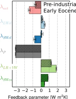
Feedbacks stabilising the climate are stronger for the early Eocene climate than for the pre-industrial case as the steeper slope of the regression line in Fig. 4 illustrates. Stronger sta-bilising feedbacks lead to a weaker warming by forests at the end of the Eocene simulation (Table 3) and to a smaller estimated equilibrium temperature response than for pre-industrial conditions. This result is surprising because the simulations by Caballero and Huber (2013) indicate the op-posite result. They analyse the strength of feedbacks trig-gered by a greenhouse gas forcing for different climate states. The study shows that feedbacks stabilise a warmer climate less than a colder climate leading to a higher climate sensi-tivity in the warmer climate. Presumably, the feedbacks as-sociated with a response to an increase in greenhouse gas concentration cannot directly be compared with feedbacks arising from a response to changes in land surface.
We analyse the single components of the net feedback to identify the reason for the different strengths in net feedback in both climate states. The short-wave clear-sky feedback pa-rameter,λSWcs, is significantly smaller for the early Eocene
climate than for pre-industrial conditions (Fig. 7). This feed-back mainly refers to changes in the sea-ice cover and snow cover together with the short-wave contribution of the water-vapour feedback. We expect that the ice-albedo feedback is weak for the early Eocene climate because permanent sea-ice is absent and snow occurs only seasonally. The smallλSWcs
agrees with this expectation. Also the zonal mean tempera-ture difference between the forest world and the desert world indicates a weak ice-albedo feedback because forests warm the northern high latitudes much less for the early Eocene climate than they do for pre-industrial conditions (Fig. 8).
λWV+LRlargely quantifies the sum of the negative
lapse-rate feedback and the positive water-vapour feedback. This feedback parameter is larger for the early Eocene climate than for pre-industrial conditions indicating either a weaker lapse-rate feedback, a stronger water-vapour feedback, or both. This result agrees with previous studies which find that the water-vapour feedback is stronger the warmer the climate is (Meraner et al., 2013; Loptson et al., 2014).
The largest differences in the feedback parameters ap-pear in the short-wave cloud feedback parameter, λSWcl,
which is−0.8 W m−2K−1for the early Eocene climate and 0.1 W m−2K−1 for the pre-industrial climate. Even
consid-ering the large uncertainty in the estimate,λSWcldiffers
sig-nificantly between the early Eocene and pre-industrial con-ditions. The cloud albedo feedback is stronger and of oppo-site sign for the early Eocene climate than for pre-industrial conditions.λSWcl, however, also includes masking effects of
clouds which weakens the result on the climate-dependent cloud albedo feedback.
To identify the reason for the different sign inλSWclfor the
cold and warm climates considered here, we analyseλSWcl
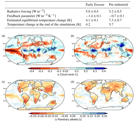
Table 3.Net radiative forcing by afforesting a bright desert world for the early Eocene climate and the pre-industrial climate. Further, the net feedback parameter and the equilibrium temperature change are listed. The values are derived from the comparison of the respective forest world with the respective bright desert world using the linear regression approach (Sect. 3.1). The estimated equilibrium temperature change is based on Eq. (6). The 95 % confidence interval is given. The transient temperature change refers to the temperature difference averaged over the last 30 years of the simulations.
Early Eocene Pre-industrial
Radiative forcing[W m−2] 5.8±0.4 5.2±0.5 Feedback parameter[W m−2K−1] −1.4±0.1 −0.7±0.1 Estimated equilibrium temperature change[K] 4.1±0.1 7.3±0.7 Temperature change at the end of the simulations[K] 4.2 5.7
Figure 6.Difference in cloud cover and planetary albedo between the forest world and the bright desert world averaged over the first year of the simulations. Differences in planetary albedo result from differences in surface albedo and in cloud cover.(a, c)show the differences for the early Eocene climate and(b, d)for the pre-industrial climate.
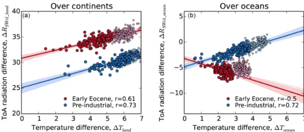
cloud radiative flux between the forest world and the bright desert world,1RSWcl, into1RSWclabove oceans and above
continents (similar to Andrews et al., 2012). We display tem-perature differences over continents with radiation differ-ences over continents (Fig. 9a). Similarly, we display tem-perature differences over oceans with radiation differences over oceans (Fig. 9b).
Over the continents, λSWclis nearly of the same strength
in both climate states as the slopes of the regression lines in Fig. 9a illustrate. Over the oceans, however, λSWcl is
pos-itive for pre-industrial conditions and negative for the early Eocene climate (Fig. 9b). The opposite sign inλSWclover the
ocean indicates that presumably, a different structure in cloud cover changes in both climates (see Fig. 6) is the reason for a state-dependent cloud feedback in our simulations.
A state-dependent cloud feedback is also suggested by Goldner et al. (2013) who estimate the climate sensitiv-ity to the Antarctic ice sheet in today’s climate and in the
Eocene climate. Their simulations suggest that the Antarc-tic ice sheet cools both climates. Changes in low clouds am-plify the cooling in the Eocene climate, while changes in low clouds dampen the cooling in modern climate. Despite the agreement with Goldner et al. (2013), we have to interpret our results with caution because cloud feedbacks are highly model-dependent (Randall et al., 2007; Dufresne and Bony, 2008). As a further word of caution, we should remember that the Gregory approach includes the assumption that feed-backs act linearly. Figure 9b, however, indicates that the TOA cloud short-wave radiation seems to evolve non-linearly with temperature in the early Eocene. We are currently not able to explain this behaviour.
4.2 Forestation of a dark desert world
Table 4.Net radiative forcing by afforesting a dark desert world for the early Eocene climate and for pre-industrial conditions. Further, the net feedback parameter and the equilibrium temperature change are listed. The values are derived from the comparison of the respective forest world with the respective dark desert world using the linear regression approach (Sect. 3.1). The estimated equilibrium temperature change is based on Eq. (6). The 95 % confidence interval is given. The temperature change at the end on the simulations considers the average over the last 30 years of the simulation.
Early Eocene Pre-industrial
Radiative forcing[W m−2] −3.4±0.4 −3.1±0.5 Feedback parameter[W m−2K−1] −0.7±0.1 −0.8±0.2 Estimated equilibrium temperature change[K] −5.3±0.6 −3.8±0.5 Temperature change at the end of the simulations[K] −4.2 −3.0
−3 −2 −1 0 1 2 3
Feedback parameter [W m K]-2
Pre-industrial
Early Eocene
λ
netλ
LWclλ
SWclλ
Pλ
LR +VWλ
SWcsFigure 7.Net feedback parameter and its single components for the comparison of the forest world to the bright desert world. Hatched and plain bars show the feedback parameters for the pre-industrial climate and the early Eocene climate, respectively. The error bars refer to the 95 % confidence interval.
3.0 K until the end of the early Eocene simulations and until the end of the pre-industrial simulations, respectively (Ta-ble 4). The cooling results from a negative radiative forc-ing of about 3 W m−2 in both climate states (Fig. 10). The main contributor to the net radiative forcing is the short-wave cloud component1QSWcl(Fig. 11) which amounts to about
−5 W m−2in both climates. The negative1Q
SWclillustrates
that forests cool the dark desert world by increasing cloud cover.
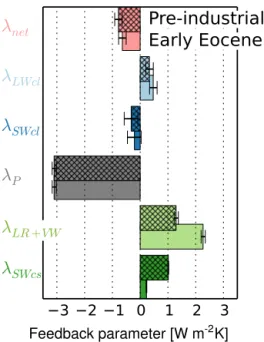
The individual feedbacks are of different strengths for the early Eocene climate and for pre-industrial conditions (Fig. 12). The combined lapse-rate and water-vapour feed-back, λLR+VW, is larger for the early Eocene climate than
for pre-industrial conditions, while the short-wave clear-sky component, λSWcs, is smaller for the early Eocene climate.
The larger λLR+VW for the early Eocene climate indicates
-90 -45
-15
0
15
45
90
Latitudes [ N]
◦0
2
4
6
8
10
12
14
Te
mp
era
tur
e d
iffe
ren
ce
[K
]
Pre-industrial Early Eocene
Figure 8.Zonal mean temperature difference between the forest world and the desert world. Red line and blue line refer to the early Eocene climate and the pre-industrial climate, respectively. The av-erage over the last 30 years of the simulation is considered.
a stronger lapse-rate and water-vapour feedback which am-plifies the cooling by forests on a global scale. The smaller
λSWcs can likely be attributed to a weaker sea-ice albedo
feedback which leads to a weaker polar amplification of the cooling by forests than for pre-industrial conditions.
5 Conclusions
Figure 9.Evolution of the difference in TOA short-wave cloud radiative flux,RSWcl, with differences in near-surface temperature between the forest world and the bright desert world. The evolution ofRSWcl is separated in the evolution above the continents(a)and above the oceans(b). Global annual-mean values are considered. Red and blue points relate to the early Eocene climate and to the pre-industrial climate, respectively. Dark large points and bright small points show the first 150 years and the last 250 years, respectively. The regression and the correlation coefficient,r, consider the first 150 years. The shaded areas refer to the 95 % confidence interval for the regression lines.
−6 −5 −4 −3 −2 −1 0
Temperature difference [K],
∆T
−3.5
−2.5
−1.5
−0.5
T
o
A
r
a
d
ia
ti
o
n
d
if
fe
re
n
c
e
[
W
m
],
-2
∆
R
Early Eocene, r=-0.63
Pre-industrial, r=-0.53
Figure 10.Evolution of differences in the TOA radiative flux be-tween the forest world and the dark desert world with corresponding temperature differences. Global annual mean values are considered. Red and blue points relate to the early Eocene climate and to the pre-industrial climate, respectively. The first 150 years are shown and considered for the regression and the correlation coefficient,r. The shaded areas refer to the 95 % confidence interval for the re-gression lines.
the sea-ice albedo feedback amplifies warming in the north-ern high latitudes.
In the nearly ice-free, warm climate of the early Eocene, we find a similar radiative forcing by forests as in the pre-industrial interglacial climate. Climate feedbacks, however, differ considerably. The sea-ice albedo feedback is weaker for the early Eocene climate than for the pre-industrial cli-mate leading to a weaker warming by forests in the northern high latitudes. The positive lapse-rate and water-vapour feed-back is stronger than for pre-industrial conditions. Negative cloud-related feedbacks, however, are also stronger than for pre-industrial conditions and nearly outweigh the stronger positive lapse-rate and water-vapour feedback. In total,
cli--10 0 10
Radiative forcing [W m-2]
Pre-industrial
Early Eocene
Q
netQ
LWclQ
SWclQ
LWcsQ
SWcsFigure 11.Net radiative forcing and its single components for the comparison of the forest world to the dark desert world. The hatched and the plain bars show the radiative forcings for the pre-industrial climate and the early Eocene climate, respectively. The error bars refer to the 95 % confidence interval.
mate feedbacks stabilising the global climate are stronger for the early Eocene climate than for the pre-industrial case, and forests warm the Eocene climate to a lesser degree than the pre-industrial climate.
−3 −2 −1 0 1 2 3
Feedback parameter [W m-2K]
Pre-industrial
Early Eocene
λ
netλ
LWclλ
SWclλ
Pλ
LR +VWλ
SWcsFigure 12.Net feedback parameter and its single components for the comparison of the forest world to the dark desert world. The hatched and the plain bars show the feedback parameters for the pre-industrial climate and the early Eocene climate, respectively. The error bars refer to the 95 % confidence interval.
for the early Eocene climate results in a stronger global cool-ing than in pre-industrial climate, and a much weaker snow and ice-albedo feedback leads to a weaker high-latitude cool-ing for the early Eocene climate than for pre-industrial con-ditions.
In the real world, the values of surface albedo are within the range of the values prescribed in our sensitivity study. In most regions the surface albedo is much closer to the low value of 0.1 than to the high value. Only in some desert re-gions with desiccated palaeo lakes, like the Bodélé depres-sion in North Africa today, values are as high as 0.4. We assume that this is valid also for the Early Eocene climate. Therefore, we assume that our results for dark soil are ap-plicable to the real world qualitatively albeit with a smaller amplitude of values.
Even though we have presented results from only one model, we assume that our main conclusion – that radiative forcing varies little with the climate state, while subsequent feedbacks depend on the climate state – is valid in general. A weak snow/ice albedo feedback in an almost ice-free cli-mate is what we expect other models to reproduce. A stronger water-vapour feedback in a warmer climate is consistent with previous studies using another model (Loptson et al., 2014). Our results on cloud feedbacks, however, are likely model-dependent because cloud feedbacks differ among models in general (Randall et al., 2007; Dufresne and Bony, 2008).
In our study, plant functional types are considered to be the same for the early Eocene climate as for the pre-industrial climate. We assume that this simplification will only weakly
affect the results of our study, at least in the qualitative sense. We prescribe extreme land cover differences between com-pletely forested and comcom-pletely deserted continents. This dif-ference presumably causes much stronger effects than the difference in the physiology between current forests and early Eocene forests. The topic of changing plant functional types with climate will be subject to further studies.
Acknowledgements. We are grateful for comments by Bjorn Stevens and Thorsten Mauritsen, and we thank Veronika Gayler and Helmuth Haak for technical support. Comments by two anonymous reviewers which improved this paper are greatly appreciated. This work used computational resources by Deutsches Klima Rechenzentrum (DKRZ) and was supported by the Max Planck Gesellschaft (MPG).
The article processing charges for this open-access publication were covered by the Max Planck Society.
Edited by: M. Crucifix
References
Alkama, R., Kagayama, M., and Ramstein, G.: A sensitivity study to global desertification in cold and warm climates: Results from IPSL OAGCM model, Clim. Dynam., 38, 1629–1647, doi:10.1007/s00382-011-1101-6, 2012.
Andrews, T., Gregory, J., Webb, M., and Taylor, K.: Forcing, feed-backs and climate sensitivity in CMIP5 coupled atmosphere-ocean climate models, Geophys. Res. Lett., 39, L09712, doi:10.1029/2012GL051607, 2012.
Bathiany, S., Claussen, M., Brovkin, V., Raddatz, T., and Gayler, V.: Combined biogeophysical and biogeochemical effects of large-scale forest cover changes in the MPI earth system model, Bio-geosciences, 7, 1383–1399, doi:10.5194/bg-7-1383-2010, 2010. Beerling, D. and Royer, D.: Convergent Cenozoic CO2history, Nat.
Geosci., 4, 418–420, doi:10.1038/ngeo1186, 2011.
Betts, A. K. and Ball, J. H.: Albedo over the boreal forest, J. Geo-phys. Res.-Atmos., 102, 28901–28909, doi:10.1029/96JD03876, 1997.
Bice, K. L. and Marotzke, J.: Numerical evidence against reversed thermohaline circulation in the warm Paleocene/Eocene ocean, J. Geophys. Res., 106, 11529–11542, 2001.
Bijl, P. K.: Early Palaeogene temperature evolution of the southwest Pacific Ocean, Nature, 461, 776–779, doi:10.1038/nature08399, 2009.
Bonan, G. B.: Effects of boreal forest vegetation on global climate, Nature, 359, 716–718, 1992.
Bonan, G. B.: Forests and Climate Change: Forcings, Feedbacks, and the Climate Benefits of Forests, Science, 320, 1444–1449, 2008.
Caballero, R. and Huber, M.: State-dependent climate sensitiv-ity in past warm climates and its implications for future cli-mate projections, P. Natl. Acad. Sci. USA, 110, 14162–14167, doi:10.1073/pnas.1303365110, 2013.
Claussen, M., Brovkin, V., and Ganopolski, A.: Biogeophysical ver-sus biogeochemical feedbacks of large-scale land cover change, Geophys. Res. Lett., 28, 1011–1014, 2001.
Dufresne, J. and Bony, S.: An Assessment of the Primary Sources of Spread of Global Warming Estimates from Coupled Atmosphere-Ocean Models, J. Climate, 21, 5135–5144, 2008. Fraedrich, K., Jansen, H., Kirk, E., and Lunkeit, F.: The Planet
Sim-ulator: Green planet and desert world, Meteorol. Z., 14, 305–314, doi:10.1127/0941-2948/2005/0044, 2005.
Goldner, A., Huber, M., and Caballero, R.: Does Antarctic glacia-tion cool the world?, Clim. Past, 9, 173–189, doi:10.5194/cp-9-173-2013, 2013.
Gregory, J., Ingram, W., Palmer, M., Jones, G., and Stott, P.: A new method for diagnosing radiative forcing and climate sensitivity, Geophys. Res. Lett., 31, L03205, doi:10.1029/2003GL018747, 2004.
Heinemann, M., Jungclaus, J. H., and Marotzke, J.: Warm Pale-ocene/Eocene climate as simulated in ECHAM5/MPI-OM, Clim. Past, 5, 785–802, doi:10.5194/cp-5-785-2009, 2009.
Huber, M. and Caballero, R.: The early Eocene equable climate problem revisited, Clim. Past, 7, 603–633, doi:10.5194/cp-7-603-2011, 2011.
Hutchison, J.: Turtle, crocodilian, and champsosaur diversity changes in the Cenozoic of the north-central region of western United States, Palaeogeogr. Palaeocl., 37, 149–164, doi:10.1016/0031-0182(82)90037-2, 1982.
Ilyina, T., Six, K. D., Segschneider, J., Maier-Reimer, E., Li, H., and Nunez-Riboni, I.: Global ocean biogeochemistry model HAMOCC: Model architecture and performance as component of the MPI-Earth System Model in different CMIP5 experi-mental realizations, J. Adv. Model. Earth Syst., 5, 287–315, doi:10.1029/2012MS000178, 2013.
Ivany, L., Simaeys, S. V., Domack, E., and Samson, S.: Evidence for an earliest Oligocene ice sheet on the Antarctic Peninsula, Geology, 34, 377–380, doi:10.1130/G22383.1, 2006.
Jungclaus, J. H., Fischer, N., Haak, H., Lohmann, K., Marotzke, J., Matei, D., Mikolajewicz, U., Notz, D., and von Storch, J. S.: Characteristics of the ocean simulations in the Max Planck Insti-tute Ocean Model (MPIOM) the ocean component of the MPI-Earth system model, J. Adv. Model. MPI-Earth Syst., 5, 422–446, doi:10.1002/jame.20023, 2013.
Li, C., von Storch, J.-S., and Marotzke, J.: Deep-ocean heat up-take and equilibrium climate response, Clim. Dynam., 40, 1071– 1086, doi:10.1007/s00382-012-1350-z, 2012.
Liakka, J., Colleoni, F., Ahrens, B., and Hickler, T.: The im-pact of climate-vegetation interactions on the onset of the Antarctic ice sheet, Geophys. Res. Lett., 41, 1269–1276, doi:10.1002/2013GL058994, 2014.
Loptson, C. A., Lunt, D. J., and Francis, J. E.: Investigating vegetation-climate feedbacks during the early Eocene, Clim. Past, 10, 419–436, doi:10.5194/cp-10-419-2014, 2014.
Lunt, D. J., Jones, T. D., Heinemann, M., Huber, M., LeGrande, A., Winguth, A., Loptson, C., Marotzke, J., Roberts, C. D., Tin-dall, J., Valdes, P., and Winguth, C.: A model-data comparison for a multi-model ensemble of early Eocene atmosphere-ocean simulations: EoMIP, Clim. Past, 8, 1717–1736, doi:10.5194/cp-8-1717-2012, 2012.
Markwick, P.: Equability, continentality, and tertiary cli-mate – the crocodilian perspective, Geology, 22, 613–616, doi:10.1130/0091-7613(1994)022<0613:ECATCT>2.3.CO;2, 1994.
Meraner, K., Mauritsen, T., and Voigt, A.: Robust increase in equi-librium climate sensitivity under global warming, Geophys. Res. Lett., 40, 5944–5948, doi:10.1002/2013GL058118, 2013. Otto-Bliesner, B. L. and Upchurch, G. R.: Vegetation-induced
warming of high-latitude regions during the late Cretaceous pe-riod, Nature, 385, 804–807, 1997.
Pearson, P., van Dongen, B., Nicholas, C., Pancost, R., and Schouten, S.: Stable warm tropical climate through the Eocene Epoch, Geology, 35, 211–214, 2007.
Port, U., Brovkin, V., and Claussen, M.: The influence of vegetation dynamics on anthropogenic climate change, Earth Syst. Dynam., 3, 233–243, doi:10.5194/esd-3-233-2012, 2012.
Raddatz, T. J., Reick, C. H., Knorr, W., Kattge, J., Roeckner, E., Schnur, R., Schnitzler, K.-G., Wetzel, P., and Jungclaus, J.: Will the tropical land biosphere dominate the climate-carbon cycle feedback during the twenty-first century?, Clim. Dynam., 29, 565–574, 2007.
Randall, D. A., Wood, R. A., Bony, S., Colman, R., Fichefet, T., Fyfe, J., Kattsov, V., Pitman, A., Shukla, J., Srinivasan, J., Stouf-fer, R. J., Sumi, A., and Taylor, K. E.: Climate models and their evaluation, in: Climate change 2007: The physical basics. Contri-bution of working group I to the Fourth Assessment Report of the Intergovernmental Panel on Climate Change, Cambridge Univer-sity Press, Cambridge, UK and New York, NY, USA, 589–662, 2007.
Reick, C. H., Raddatz, T., Brovkin, V., and Gayler, V.: Rep-resentation of natural and anthropogenic land cover change in MPI-ESM, J. Adv. Model. Earth Syst., 5, 459–482, doi:10.1002/jame.20022, 2013.
Sewall, J. O., Sloan, L. C., Huber, M., and Wing, S.: Climate sen-sitivity to changes in land surface characteristics, Global Planet. Change, 26, 445–465, 2000.
Sluijs, A., Schouten, S., Pagani, M., Woltering, M., Brinkhuis, H., Sinninghe Damste, J. S., Dickens, G. R., Huber, M., Reichart, G., Stein, R., Matthiessen, J., Lourens, L. J., Pedentchouk, N., Back-man, J., Moran, K., and the Expedition 302 Scientists: Subtrop-ical Arctic Ocean temperatures during the Palaeocene/Eocene thermal maximum, Nature, 441, 610–613, 2006.
Stevens, B., Giorgetta, M., Esch, M., Mauritsen, T., Crueger, T., Rast, S., Salzmann, M., Schmidt, H., Bader, J., Block, K., Brokopf, R., Fast, I., Kinne, S., Kornblueh, L., Lohmann, U., Pin-cus, R., Reichler, T., and Roeckner, E.: Atmospheric component of the MPI-M Earth System Model: ECHAM6, J. Adv. Model. Earth Syst., 5, 146–172, doi:10.1002/jame.20015, 2013. Warner, T. T.: Desert Meteorology, Cambridge University Press,
Wilf, P.: When are leaves good thermometers? A new case for leaf margin analysis, Paleobiology, 23, 373–390, 1997.
Wolfe, J.: Paleoclimatic estimates from Tertiary leaf assemblages, Annu. Rev. Earth Planet Sci., 23, 119–142, 1995.
Zachos, J., Berza, J., and Wise, S.: Early Oligocene ice-sheet expansion on Antarctica – Stable isotope and sed-imentological evidence from Kerguelen Plateau southern Indian-Ocean, Geology, 20, 569–573, doi:10.1130/0091-7613(1992)020<0569:EOISEO>2.3.CO;2, 1992.