www.atmos-chem-phys.net/11/1505/2011/ doi:10.5194/acp-11-1505-2011
© Author(s) 2011. CC Attribution 3.0 License.
Chemistry
and Physics
Quantifying immediate radiative forcing by black carbon and
organic matter with the Specific Forcing Pulse
T. C. Bond1, C. Zarzycki1, M. G. Flanner2, and D. M. Koch3
1Department of Civil and Environmental Engineering, University of Illinois at Urbana-Champaign, Urbana, Illinois, USA 2Department of Atmospheric, Oceanic and Space Sciences, University of Michigan Ann Arbor, Michigan, USA
3NASA Goddard Institute for Space Studies, Columbia University, New York, USA Received: 18 May 2010 – Published in Atmos. Chem. Phys. Discuss.: 28 June 2010 Revised: 12 November 2010 – Accepted: 11 January 2011 – Published: 16 February 2011
Abstract. Climatic effects of short-lived climate forcers (SLCFs) differ from those of long-lived greenhouse gases, because they occur rapidly after emission and because they depend upon the region of emission. The distinctive tem-poral and spatial nature of these impacts is not captured by measures that rely on global averages or long time integra-tions. Here, we propose a simple measure, the Specific Forc-ing Pulse (SFP), to quantify climate warmForc-ing or coolForc-ing by these pollutants, where we define “immediate” as occurring primarily within the first year after emission. SFP is the amount of energy added to or removed from a receptor re-gion in the Earth-atmosphere system by a chemical species, per mass of emission in a source region. We limit the applica-tion of SFP to species that remain in the atmosphere for less than one year. Metrics used in policy discussions, such as total forcing or global warming potential, are easily derived from SFP. However, SFP conveys purely physical informa-tion without incurring the policy implicainforma-tions of choosing a time horizon for the global warming potential.
Using one model (Community Atmosphere Model, or CAM), we calculate values of SFP for black carbon (BC) and organic matter (OM) emitted from 23 source-region com-binations. Global SFP for both atmosphere and cryosphere impacts is divided among receptor latitudes. SFP is usually greater for open-burning emissions than for energy-related (fossil-fuel and biofuel) emissions because of the timing of emission. Global SFP for BC varies by about 45% for energy-related emissions from different regions. This varia-tion would be larger except for compensating effects. When emitted aerosol has larger cryosphere forcing, it often has lower atmosphere forcing because of less deep convection and a shorter atmospheric lifetime.
Correspondence to:T. C. Bond ([email protected])
A single model result is insufficient to capture uncer-tainty. We develop a best estimate and uncertainties for SFP by combining forcing results from 12 additional mod-els. We outline a framework for combining a large num-ber of simple models with a smaller numnum-ber of enhanced models that have greater complexity. Adjustments for black carbon internal mixing and for regional variability are dis-cussed. Emitting regions with more deep convection have greater model diversity. Our best estimate of global-mean SFP is +1.03±0.52 GJ g−1 for direct atmosphere forcing of black carbon, +1.15±0.53 GJ g−1 for black carbon in-cluding direct and cryosphere forcing, and−0.064 (−0.02, −0.13) GJ g−1 for organic matter. These values depend on the region and timing of emission. The lowest OM:BC mass ratio required to produce a neutral effect on top-of-atmosphere direct forcing is 15:1 for any region. Any lower ratio results in positive direct forcing. However, important processes, particularly cloud changes that tend toward cool-ing, have not been included here.
1 Introduction
Atmospheric burdens of chemical species with short atmo-spheric lifetimes respond rapidly to changes in emission. Many of these species, such as aerosols or the precursors of ozone, affect the Earth’s radiative balance, either di-rectly or by interacting with atmospheric chemistry. The ra-diative response to emissions of these “short-lived climate forcers” (SLCFs) differs greatly from the response to long-lived greenhouse gases, for which atmospheric burdens and the resulting forcing lag emission changes by decades.
Because mitigation of SLCFs could rapidly reduce cli-mate warming, the possibility of decreasing them has en-gendered a flurry of interest (Hansen et al., 2000; Grieshop et al., 2009). SLCFs emitted from some locations also impact sensitive regions such as the Arctic (Quinn et al., 2008). However, the impact and, hence, the value of such regionally-dependent reductions has been difficult to express using traditional measures of climate change. For example, global warming potentials (GWPs) are discussed for pur-poses of trading, and have been estimated for some short-lived species, but they do not communicate explicit informa-tion on either the timing or locainforma-tion of climate impact.
In this paper, we propose a method for quantifying tem-poral and regional climate impacts of SLCFs, a first step to-ward valuation. In Sect. 2, we introduce the Specific Forcing Pulse (SFP) to quantify both location and immediacy. We do not propose that SFP should be used to equate the impacts of greenhouse gases and SLCFs, which operate over funda-mentally different temporal and spatial scales. Nevertheless, in Sect. 2, we also discuss the connection between SFP and other common measures of climate impact, such as GWPs and total radiative forcing.
Section 3 presents values of SFP for black carbon (BC) and organic matter (OM) aerosol emitted from several source regions, derived using one chemical transport model. We discuss reasons for differences among regions. We also ac-knowledge that reliance on a single model is insufficient. In Sect. 4, we therefore propose a method of deriving a best es-timate and uncertainties for SFP by adjusting our SFP with an ensemble of other modeled values. Finally, Sect. 5 com-pares the values derived in this work with previous estimates of radiative forcing and GWP.
2 Specific Forcing Pulse
2.1 The distinct nature of immediate forcing
We define “immediate forcing” as a condition in which there is no delay between emission and the delivery of the en-tire forcing impact attributable to that emission. Although forcing is never truly immediate, we argue that it may be considered so when the entire impact occurs within a very short period after emission. The definition of “short” is
ar-bitrary, but we propose thatone year is a reasonable time limit. With this definition, species with e-folding lifetimes of four months produce immediate forcing, because 95% of the forcing occurs within one year after emission. One might argue with this choice of time limit: why not three, five, or ten years? However, this selection is not important. Climate-forcing agents that have major impacts in the current Earth system happen to have lifetimes that are either shorter than one year or much longer. A one-year time limit effectively divides species that have impacts only in the very near future and those for which accumulated burdens are important.
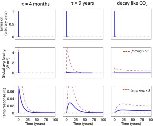
Changes in radiative forcing can often be represented us-ing just a few characteristic time scales. For example, Wild et al. (2001) showed that a pulse of emitted nitrogen oxide caused climate forcing through its interactions with tropo-spheric ozone (lifetime less than one year) and with methane (lifetime greater than 8 years). Like species that interact solely with the ozone chemical system, aerosols alter forcing shortly after emission, and this forcing dies away within a short time when the species no longer interact with radiation. Figure 1 shows the time evolution of forcing and cli-mate response by pulse emissions of different hypothetical species. The left panels show an SLCF with ane-folding time of four months. Middle panels show a substance with a lifetime similar to that of methane (9 years). The right panels show a substance with an atmospheric decay similar to that of CO2. The top panels in Figure 1 are of arbitrary scale and in-dicate that all species here are introduced as pulse emissions. The middle panels show forcing by each species, with mag-nitudes scaled so that the integrated forcing over 100 years is identical for each substance. Compared with the longer-lived species, forcing by SLCFs appears as a pulse of forcing or a burst of energy, although its lifetime is non-zero. Re-sponse to this immediate forcing is very different from re-sponse to longer-lived species. The bottom graphs in Fig. 1 show climate response to each time series of forcing, using the equations provided by Boucher and Reddy (2008). The figures show that the temporal evolution of forcing affects temperature response to a pulse emission. (For this reason, Global Temperature Potentials differ from Global Warming Potentials; see Shine et al., 2005).
Because the timing of forcing is important, it is worthwhile to conduct separate investigations for species that have dis-tinctly different time scales. In this paper, we explore meth-ods of quantifying the impacts of climate-forcing agents that provide immediate forcing.
2.2 Regional dependence of forcing
Fig. 1.Forcing and response to pulse emissions of hypothetical substances with different atmospheric lifetimes. Each trace is discontinued when the signal drops below 10−5of the peak value of the short-lived forcer. Forcing (middle panels) has been scaled so that the area under each of three curves is identical over 100 years. Dashed red trace shows forcing value times 50 to show more detail in the time dependence. Temperature response (lower panels) is estimated with the relationship and parameters given by Boucher and Reddy (2007), and assumes that spatial dependence of forcing is similar to that of CO2.
the United States and from Africa. (The model used to create this figure is discussed further in Sect. 3).
The forcing exerted upon specific regions of interest (re-ceptor regions) also depends on the emitting region. Here, we choose latitude bands as the receptor regions, and these are shown in Fig. 2 with dashed lines. Hansen et al. (1997) showed that climate response is approximately proportional to forcing at specific latitudes, regardless of the nature of the forcing. Shindell and Faluvegi (2009) apportioned tempera-ture responses in the Arctic to forcing within specific latitude bands. Koch et al. (2007) calculated forcing both attributed to specific regions and acting upon specific regions. Here, we provide a formal framework to quantify this spatial nonuni-formity as it relates to both emission and receptor regions.
2.3 Definition of the Specific Forcing Pulse
We define the Specific Forcing Pulse SFPS
E as the
en-ergy added to the Earth-atmosphere system by one gram of speciesS emitted in regionE, during its entire lifetime. We further define the SFP for energy added within a region, SFPS
E(Rj), as the energy added to a regionRj by one gram
ofS emitted in regionE. The units of SFP are joules per gram emitted. SFP provides a policy-relevant measure:
ben-efit, or disbenben-efit, per mass emitted – the “bang for the buck.” The formal equation is:
SFPSE(Rj)=
1 ME,s 0
Z ϕ2
ϕ1 Z θ2
θ1 Z 1yr
t=0
fES(θ,ϕ,t )bES(θ,ϕ,t )
ρ2earthcosθ dθ dϕdt (1) wherefESis the net change in the rate of energy input per mass ofSin the system (W g−1);bS
E is the column burden or
surface loading (g m−2)of the substance at (θ,ϕ) remaining at timet from an emission pulse of magnitudeME,0(g) in regionE,ϕ1 andϕ1are the longitude boundaries ofR,θ1 andθ2are the latitude boundaries ofR, andρearthis the ra-dius of the Earth. The subscriptEis included forf andb because the characteristics of speciesSwithin regionRmay differ with emitting region. The upper integral limit of one year comes from our definition of immediacy in the previous section.
Fig. 2.Demonstration of forcing by BC emitted in a specific region, exerted upon other receptor regions. Here, the receptor regions are latitude bands. Maps to the left show total forcing from energy-related emissions in the United States (top) and open biomass burn-ing in Africa (bottom). Figures to the right show zonal integrals of forcing, normalized to emissions. SFP is the integral over lati-tudes of interest. Shading in the right graphs shows two examples:
SFPBCUSen(30◦–60◦N) andSFPBCAfrOpen(0◦–30◦N).
right show zonal integrals of the forcing, normalized by to-tal regional emissions. There are marked differences in the latitudinal dependence of forcing by emissions from each re-gion. Two examples of SFP calculation are marked in the figure: SFPBCUSen(30◦–60◦N) and SFPBC
AfrOpen(0◦–30◦N). This forcing assumes present-day spatial distribution of emission. We propose that energy (joules) added to a specific region, rather than power (watts, energy per time) or radiative forc-ing (watts per area), is a basic measure for forcforc-ings that begin and end rapidly. While other impacts are best quantified in terms of forcing integrated over time, with units of W yr, units of J indicate that SLCF forcings are fundamentally dif-ferent. They are better represented as delta functions, charac-terized by an area under a curve rather than the curve’s height or width. For a true delta function, the integral is identical for any upper limit of the time integral, ranging from a small time step to infinity. The term “pulse” may also be used when any reasonable choice of the integral limit yields an identical result, as it does for SLCFs.
The pulse representation is limited to climate forcers with relatively short lifetimes. For CO2, integrated forcing during the first year after emission is less than 2% of the integrated forcing over 100 years, so this forcing does not occur as a pulse. While SFP is appropriate for short-lived species, the effects of longer-lived species should be described as inte-grated forcing. Impacts of species that act on both short-lived and long-lived components, such as carbon monoxide acting on ozone and methane, might be partitioned into two compo-nents: a pulse and an integrated forcing.
By convention, the term “forcing” is usually defined with regard to the net perturbation at the top of the atmosphere (TOA). We will present TOA values here unless otherwise stated, but we will also show that the concept of SFP can be used to communicate other changes in energy balance (see Sect. 3.3).
2.4 Connection between SFP and modeled forcing
Although global chemical-transport models usually do not use pulse emission functions, SFP can be determined from their output, with some limitations. An explanation that uses a first-order box model is given in Appendix A (Supplement). Annually-averaged values of SFP can be determined from models with constant emission rates as the ratio of forcing to emission, with a change in units. This calculation is pos-sible only for short-lived species, for which burdens are in equilibrium with emissions.
The box-model derivation also shows that SFP is the prod-uct of forcing per mass (fS)and lifetime (τs). These two values can aid in diagnosing reasons for differences in SFP among seasons or regions.
2.5 Connection between SFP and global warming potentials
In this paper, we present SFP to quantify forcing that de-pends on the regions of emission and of forcing. Such quan-tification may lead to a better understanding of the bene-fits (or costs) of reducing SLCF emissions. We do not pro-pose SFP as a trading metric here, as it captures impacts that cannot be reflected in globally-averaged, integrated metrics. However, many discussions about mitigating climate-active species require trading metrics such as Global Warming Po-tentials (GWPs). Because of this history, we draw connec-tions between SFP and more traditional measures such as GWP.
2.5.1 Absolute global warming potential
units of AGWP are W m−2yr g−1. Its definition can be written:
AGWPS(H ) 1 M0S
Z H
0
fsbs(t )dt (2) where H is a chosen time horizon and all other vari-ables are as in Eq. (1). SFP has some important differences from AGWP, and we propose it to provide quantification that AGWP cannot.
Regionality.SFP refers to forcing within a specific region, not a global average. However, the global sum of SFP (with a change in units) equates to AGWP. For such regional energy flows, SFP must have either units of power (W) or energy (J) instead of forcing units (W m−2), because the latter are not conservative. Fasullo and Trenberth (2008) use watts for regional energy flows in an energy-balance model; we choose joules to express the integral nature of the pulse.
Timing of forcing.When a value is presented as SFP, it is clear that the forcing occurs immediately, by our definition of the word.
Representativeness of steady state.SFP can be multiplied by emission rate to obtain annual forcing, while the same is not true of AGWP for longer-lived pollutants.
Independence of time horizon.We limit the use of SFP to forcings that are effectively pulses, so that a one-year time integral captures 95% of the forcing for short-lived species. Although the upper limit of the time integral in Eq. (1) is one year, the same answer would result from any longer value of the time horizon. This means that SFP does not depend on the value ofH for any reasonable choice. In contrast, the value of AGWP remains ambiguous untilHis chosen. That is,
1 Aearth
X
j
SFPs(Rj)=AGWPs(H ) (3)
for any value ofH.
We have also chosen some different terminology. We avoid the term “global warming” because SFP is neither global nor required to produce warming. We identify the SFP as a “pulse” rather than a “potential” because it is not referenced to a chosen substance, as are global warming po-tentials and ozone depletion popo-tentials. Finally, we choose the term “specific” to have the same meaning as in “specific heat”: the sense of forcing per mass. The term is included as a reminder that the determination of total forcing for SLCFs is inseparable from emission rate.
2.5.2 Global warming potential
The currency of climate mitigation discussions is presently “carbon equivalence” using the global warming potential (GWP), which is defined as:
GWPs(H )= RH
0 fsms(t )dt RH
0 fCO2mCO2(t )dt
(4)
The denominator gives the amount of forcing by CO2 dur-ing the time horizonH, and the numerator is both the AGWP and the global sum of regional SFPs, so that
GWPs(H )= AGWP s(H )
AGWPCO2(H )= P
jSFPs(Rj)
Aearth·AGWPCO2(H ) (5) The choice ofH reflects the value of future climate bene-fits, and the time horizon amounts to a value judgment about the importance of future forcing. Current negotiations use H= 100 years, but others (e.g. 20 or 500 years) are also dis-cussed. The choice ofH matters only when some pollutant remains in the atmosphere at the end of the time period, as is the case for CO2 but not for SLCFs. Vast differences in GWP forH= 20 years versusH= 100 years (Fuglestvedt et al., 2009) result entirely from the denominators in Eqs. (4) and (5). The use of SFP as opposed to AGWP clarifies that forcing occurs immediately and that it is all counted. SFP conveys purely physical information about forcing. It has a direct connection to policy-relevant metrics, yet it requires no choices that favor particular policies or value judgments.
A value of GWP can be obtained by dividing global SFP by a selected value for CO2 integrated forcing. Using the Bern carbon model to represent life cycle,aCO2from IPCC’s Fourth Assessment Report (chp 2), and a zero discount rate for future forcing, the value of the denominator in Eq. (5) is 1.4×10⁻³GJ g−1forτ= 100 years, and 4.0×10⁻⁴GJ g−1 forτ= 20 years.
2.6 Application of SFP to temperature change calculations
A primary use of SFP is connecting decisions regarding mit-igation and future emission in particular regions with the re-sulting climate forcing. The units of SFP are energy added to the Earth system per emission: joules per gram. This fundamental quantity can be used directly in energy-balance approaches to the Earth system (e.g. Murphy et al., 2009). Because it represents forcing per emission, SFP can also be used to estimate immediate forcing reductions caused by mit-igating black carbon or ozone, or decreased negative forcing (“unmasking”) due to sulfur controls. Integrated assessment models (Alcamo et al., 1994; Smith et al., 2000) can use SFP to connect predictions of SLCF emission with radiative forc-ing and climate response.
However, it is important to remember that forcing and warming are not the same. Forcing is an input to the Earth system and does not account for its response (i.e., feedbacks). SFP cannot be divided by the Earth’s heat capacity to deter-mine temperature change. Instantaneous forcing on a system that is not in equilibrium cannot be divided by climate sensi-tivity to determine temperature change, either.
signs. Shindell and Faluvegi (2009) showed that Arctic tem-perature response depended on the forcing latitude, but in a non-intuitive way. In Appendix B, we propose a method to account for the regional dependence of SFP in simple climate models. This derivation there is presented to foreshadow the need for regional SFP, a discussion that will occupy Sect. 3 and onward. Readers who expect to perform simple tem-perature change calculations using SFP should consult Ap-pendix B.
3 Single-model, regional estimates of SFP
In this section, we present values of the Specific Forcing Pulse for black carbon (BC) and organic matter (OM) par-ticles emitted from different regions, obtained from a single model. The idea of representing immediate changes in forc-ing could be used to communicate many changes in the ra-diative balance: warming or cooling of the atmosphere due to direct interaction with sunlight (dir); albedo changes in the cryosphere (snow and ice, cry); changes in warm clouds, and changes in cold or mixed clouds. We quantify only direct and cryosphere impacts here (SFPTOA,dir+cry), noting that warm-cloud and cold-warm-cloud changes could greatly alter the estimate of impact.
3.1 Model description
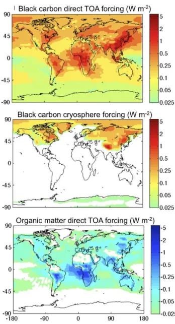
We used the Community Atmosphere Model (CAM, Collins et al., 2006), developed at the National Center for Atmo-spheric Research, to model atmoAtmo-spheric and cryoAtmo-spheric (snow and ice) forcing by black and organic carbon. Fig-ure 3 shows total forcing by BC and organic matter in the atmosphere, and by BC on snow and ice. Atmospheric temperature and pressure were prescribed from NCEP re-analysis data, strongly constraining model winds. Energy-related emissions, from year 2000 in Bond et al. (2007), were 4400 Gg yr−1 and 8900 Gg yr−1 for black and organic car-bon, respectively. Open-burning emissions from the Global Fire Emission Database, version 2 (van der Werf et al., 2006) averaged 2600 Gg yr−1and 21 000 Gg yr−1and included sea-sonality during each model year. The primary purpose of this model run is to produce values of forcing per emission, so the total values of emission are less important. Agricultural burning was not included because it appears in neither emis-sion database.
Aerosol optics were modified to reflect recent recommen-dations for black carbon (Bond and Bergstrom, 2006; Bond et al., 2006), including “coating” or internal mixing. This version of CAM does not have a full aerosol microphysical model, but the effects of coating can be approximated with higher absorption for black carbon particles that have aged. In our model, this transition has a characteristic time of about 1.2 days. The organic matter in CAM has minimal absorp-tion, ignoring the contribution of “brown” carbon, which has
Fig. 3.Forcing by black carbon in atmosphere and on snow, and by organic matter, simulated with the Community Atmosphere Model.
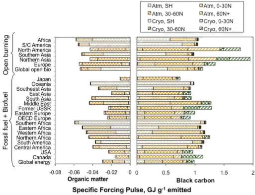
Fig. 4.Specific Forcing Pulse for BC and OM aerosol emitted from 23 region-source combinations, estimated with a single model (NCAR CCSM). SFP includes direct atmospheric and cryosphere impacts only. Note the difference in scale between the positive values for black carbon and negative values for organic matter. The single-model values presented in this figure are adjusted to reflect model ensembles in Table 1.
Emissions from 23 separate region and source combina-tions (17 energy and 6 open burning) were tagged so that concentrations and deposition at each location could be at-tributed to source regions. The 17 regions reflect the group-ings in a common integrated assessment model (IMAGE, Al-camo et al., 1994). We apportioned forcing in each model grid box (1.9◦×2.5◦) to the column burden of the aerosol
from each region. Forcing through changes in ice and snow albedo was also modeled in a separate twenty-year equilib-rium run (Flanner et al., 2009, run PD1). We apportioned this forcing to the 23 emitting regions using deposition of the tagged tracers. Global-average cryosphere forcing is +0.047 W m−2, with 20% of the total occurring in the Arctic (60◦to 90◦N).
3.2 Regional estimates of SFP for black and organic matter
Figure 4 shows SFPTOA,dir+cryfor black carbon and organic matter emitted from each 23 region-sector combination. The magnitude of each bar indicates the global SFP, or the to-tal energy added to the global atmosphere and cryosphere by one gram of emissions from that region. SFP for each region is also divided among the latitudes where forcing oc-curs, as demonstrated in Fig. 2. The apportionment of SFP into forcing regions is less certain than the global sum of SFP, because zonal transport is not well constrained and varies
among models (Textor et al., 2006), Unsurprisingly, domi-nant impacts are found at the same latitude as the region of emission.
BC has positive global SFP (warming), while the negative global SFP shows the cooling effect of reflective OM. There is more than an order of magnitude difference between the cooling per mass of OM and the warming per mass of BC; the latter is far more effective at interacting with visible ra-diation. For energy-related emissions, global SFP of BC and OM averages +0.99 and−0.030 GJ g−1, respectively. Emis-sions from open burning have higher SFPTOA: +1.13 and −0.053 GJ g−1 for BC and OM, respectively. Averages for all emissions are +1.05 GJ g−1 for BC and −0.037 GJ g−1 for OM.
The orange portion of each bar shows direct TOA forc-ing at different latitudes. These are the integrals over the latitude bands indicated in Fig. 2. For example, the diag-onally hatched portion of each bar represents energy added to the atmosphere within the Arctic (latitude 60–90◦N).
Fig. 5.Forcing-per-mass (fS)for black carbon in each month. Solid lines are global averages; dashed lines represent one standard devi-ation of the plotted regions. Arctic group (red) contains 23 regions and represents aerosol transported to the Arctic from all 23 regions. Other groups represent forcing-per-mass of all aerosol emitted from each region not located in the Arctic. NH outside Arctic (blue) con-tains 18 regions; SH outside Arctic (black) concon-tains 5 regions.
BC reduction of snow albedo (SFPcry)increases SFPTOA by about 15% on a global average. This contribution is im-portant for, but not confined to, emissions in northern re-gions: Europe, the former USSR, and North America. De-spite this cryospheforcing contribution, SFP in these re-gions is similar to that in more southerly rere-gions. Cooler regions are closer to snow, but these regions have less deep convection and the aerosol has shorter atmospheric lifetimes. The variation of SFP among regions, and the difference be-tween energy-related and open-burning SFP, is caused by seasonal and environmental differences in forcing per mass (f ) and aerosol lifetime (τ ). SFP is the product of these two factors. Figure 5 shows the seasonality offBC. For BC outside the Arctic, fBC varies by 10–40% throughout the year depending on the emitting region. AveragefBCfor extra-Arctic BC is about 40% higher in summer because the aerosol absorbs more sunlight during longer days. It also increases in summer because deep convection lofts the BC above reflective clouds, causing longerτ and greater fBC. (BC over a reflective surface has higher forcing per mass.) This seasonality explains the higher SFPBC for open burn-ing emissions compared with energy-related emissions, as the former emit preferentially during summer.
For BC within the Arctic, warming per mass is strongly seasonal. Large variations are caused much more by the availability of sunlight in the Arctic than by emitting region. Very little OM cooling occurs in the Arctic, because reflec-tive OM over a bright surface has little effect on the radiareflec-tive balance.
Even when emissions are constant in time, as they are for energy-related emissions, global SFP depends on the region of emission. There is a 45% difference among global SFPBC, and a factor of 4 difference among global SFPOCfor energy-related emissions. The diversity would be greater if Japan were included. Emissions from this island nation have a much lower SFP because of their environment, but we ne-glect it in considering diversity because the emissions are small.
3.3 Vertical energy distribution
In this paper, we mainly discuss how the addition or reduc-tion of energy by aerosols is distributed horizontally across the Earth’s surface. SFP can also represent changes in en-ergy balance in the vertical direction caused by BC absorp-tion. OM has little impact on atmospheric heating, unless it absorbs light, and it is not discussed here.
Figure 6 shows BC-SFPTOA,dir(atmospheric forcing only) for the 23 regions, this time showing the division between atmospheric heating (SFPheating)and negative forcing at the surface (SFPsurf). Top-of-atmosphere forcing is the sum of the two, and is identical to the sum of SFPTOA,dirin Fig. 4. The diversity of SFPheating among regions is similar to that of SFPTOA,dir, and biomass-burning BC again has a stronger impact per emission. Figure 6 demonstrates how BC affects energy redistribution. Each gram of emitted BC adds about 1 GJ to the Earth-atmosphere system, but that energy is dis-tributed as 2.4 GJ of increased atmospheric absorption, coun-teracted by 1.5 GJ that does not reach the surface. As the surface energy budget is relevant to determining changes in the hydrologic cycle (Chung et al., 2002; Meehl et al., 2008), SFPsurfmay also be useful for simple models.
4 Ensemble adjustments to reflect model diversity
In the previous section, we used a single model (CAM) to produce estimates of SFP for emissions from particular re-gions. Single-model estimates are insufficient because inputs and model parameterizations are uncertain. Values that re-flect a multi-model “consensus” would be preferable. How-ever, we face a challenge: no other model has estimated forc-ing for 23 regions, and few incorporate the representation of internal mixing that enhances absorption by BC.
Rather than discarding model results that lack sufficient detail for our purposes, we suggest that diversity among models is still a useful representation of uncertainty when the causes of variation are treated as explicitly as possible. Our goal is to provide best estimates and uncertainties for SFP that retains the features of our CAM estimate, includ-ing regionally-specific forcinclud-ing, but that also captures diver-sity represented by other models.
Fig. 6. SFP for black carbon, showing impact on vertical energy balance. Energy is added to atmosphere (orange bars, positive SFP) and removed from surface (green bars, negative SFP). Top of atmosphere value (black bars) is net of surface and atmosphere and is comparable to Fig. 2.
et al. (2006), to provide best estimates and uncertainties for SFP. Because most models produce only global totals for SFP, we will discuss those before developing regional esti-mates. We first outline the general approach to developing estimates from an ensemble of models (Sect. 4.1), and then describe variability in global SFP indicated by the model en-semble (Sect. 4.2). In later sub-sections, we address how aerosol mixing (Sect. 4.3), regionality (Sect. 4.4), and pole-ward transport (Sect. 4.5) affect our estimates of SFP.
4.1 General approach to simple ensemble adjustments
We separate model diversity into two categories: identi-fied andbaseline. Identified diversity can be attributed to a distinctfactor that varies between models, such as inclu-sion of a process or a change in aerosol optical properties. Baseline diversity includes the remainder of the model diver-sity and its causes remain unknown without further investi-gation. The separate treatment of individual factors is de-sirable when model representations are known to be biased and could be corrected, or when there is interest in explor-ing whether models agree on a particular effect. If a factor causes important changes in forcing, it should be isolated so observational studies can be designed to diagnose it.
We define abaselinesimulation as one in which the fac-tors of interest have similar assumptions for all models. The notion of a common baseline treatment is quite plausible, as many aerosol models use similar parameterizations of re-moval, or optical properties. Next, we defineenhancement predicted by modelm (Em)due to an identified factor (fact)
as the ratio of SFP values determined from two separate sim-ulations, one with the model’s own treatment of the factor, and one with the baseline treatment:
Em,fact=(SFPm/SFPm,base) (6) SFP for all factors predicted by modelmis then
SFPm,full=SFPm,base Y
Em,fact#n (7)
n
This equation assumes that the identified factors have mul-tiplicative effects on forcing, which is true if they affect nor-malized forcing or lifetime. We also assume that factors are independent. If they are not, then correlations must be con-sidered.
the baseline adjustment (Am,base)and the factor adjustment (Am,fact#n)suggested by modelm.
SFPm,full=SFPref,full
SFPm,base SFPref,base
Y
n
Emfact#n Eref,fact#n
=SFPref,fullAm,base Y
n
Am,fact#n (8)
The adjustments,A, are the values by which the reference model’s baseline (SFPref,full) or enhancement (Eref,fact#n) would have to be multiplied to reproduce values given by modelm.
Our goal is to combine as much information as possible from the ensemble of models to obtain a best estimate and uncertainty for SFP. However, we should also discount model results that are less realistic. If a model does not treat a factor appropriately or cannot represent it, the value of Am,fact#n for that model will be disregarded or given a lower weight. Even if a model does not represent all the desired factors properly, it can still provide a value ofAm,base, as well as otherAm,fact#n.
Finally, the best guess of SFP including uncertainty is: SFPbest=SFPref,fullAens,base
Y
n
Aens,fact#n (9)
In Eq. (11), the ensemble baseline adjustment (Aens,base) is determined by examining all values ofAm,baseto produce a central value and uncertainty. If a large number of models contributes to the estimate,Aens,basemay be the mean or me-dian value, and the uncertainty could be given by the standard deviation or interquartile range. Variation in the baseline ad-justment expresses diversity in model formulations that are not captured in any factor adjustment.
Each ensemble factor adjustment (Aens,fact#n)is developed by examining all available values ofEm,proc#n. These values may be provided by only a subset of the models. If modelm predicts the same enhancement as the reference model (i.e. Eref,fact#n=Em,fact#n), thenAm,fact#n= 1. Because of large differences in implementation within each model, it is diffi-cult to give rigid rules for choosing values forAens,proc. Sec-tion 4.2 contains the simplest demonstraSec-tion of this proce-dure.
Our proposed framework provides a more rigorous esti-mate than does simply averaging the 13 model values of SFP, because it identifies the sources of uncertainty. Division of modeled forcing into components is not a new idea; it was ex-plored by Schulz et al. (2006) and Textor et al. (2006). How-ever, this idea has not yet been carried forward to communi-cate forcing per emission. It is possible that this framework could overestimate the uncertainty in SFP, as models may contain compensating errors that allow them to match mea-surements. However, if modeled concentrations from each model are broadly consistent with observations, the diver-sity in modeled emissions, aerosol lifetimes and
forcing-per-mass represents true variability in plausible values for these parameters.
In the sections that follow, we use the values of SFP de-termined in Sect. 3 as SFPref. We first discuss the ensemble adjustmentAbase(Sect. 4.2). Sect. 4.3 discusses mixing be-tween black carbon and non-absorbing aerosol components. This process increases absorption and positive forcing, yet many models do not represent it. We also discuss variabil-ity among regions (Sect. 4.4) and Arctic transport (Sect. 4.5) to investigate whether models agree on regional variability. Other model factors could be explored in this framework. For example, the hygroscopicity of organic matter affects direct radiative forcing. However, no results from fully-sensitive models are available to provide values of the enhancement, so variability resulting from this treatment remains in the model uncertainty.
4.2 Ensemble baseline adjustment, Abase
The group of models that will be discussed here has mostly been tabulated by Schulz et al. (2006) for the AeroCom ini-tiative. This tabulation also includes results of models that did not participate in AeroCom. Models without internal mixing form the baseline ensemble. We discarded values that were later superceded by the same research group, reasoning that if the individual researchers have moved beyond their early estimates, the community should too. We also elimi-nate one model that included only clear-sky forcing (Schulz et al., 2006).
For BC forcing, the baseline ensemble includes models E, H, I, and L-S from Schulz et al. (2006), from Jones et al., 2007, (HadGEM1, +0.39 W m−2or +86 GJ g−1), and our CAM run with no internal mixing (+0.57 GJ g−1). Two mod-els may have chosen relatively high mass absorption cross-sections for BC (UIO-GCM and SPRINTARS) in an attempt to acknowledge absorption increase due to internal mixing. These were adjusted downward by the ratio between the ab-sorption cross-section for unmixed BC (7.5 m2g−1, Bond and Bergstrom, 2006) and the value used in the model to achieve a baseline value.
Figure 7 shows the cumulative distribution of modeled SFP for the 13 models. The figure also shows the value of Abase, or each model’s SFP divided by our reference value of +0.57 GJ g−1. The mean and median for SFPBCare almost identical (0.61 GJ g−1 and 0.62 Gg−1, respectively). The value ofAens,base, using the median as the best guess and the 10-th and 95-th percentiles, is 1.06±0.34. By choosing this value, we set the best guess of baseline SFP to the median of the baseline ensemble.
Fig. 7. Comparison of our baseline model results with AeroCom tabulation. Each figure shows SFPdir derived from 12 models in the AeroCom tabulation, which reported normalized direct radiative forcing and aerosol lifetime. Cumulative graphs indicate the fraction of models reporting SFPdirbelow the indicated value.Am,baseis the SFP for each model divided by SFP for the reference model (red triangle). Figure for black carbon (left) also shows the effect of internal mixing from CAM and one other model (top). Ratio between core-shell SFP and unmixed SFP indicates enhancement (Emix).
of (0.8, 2.2); the adjustment is not symmetric. There is a fac-tor of 13 difference between maximum and minimum, com-pared with a factor of two for BC. This greater disparity for OM may reflect a wider range of choices among the water uptake and light absorption properties that affect forcing.
4.3 Black carbon mixing:EmixandAmix
Mixing of black carbon with other aerosol components within individual particles (“internal mixing”) increases ab-sorption, and hence positive forcing, as first suggested by Ackerman and Toon (1981). This increase in absorption is not controversial. It has been confirmed in laboratory mea-surements (Schnaiter et al., 2005) and mixing occurs quickly after emission (Shiraiwa et al., 2007). This enhancement by mixing is already included in SFPref,full, but it is miss-ing from many published model results. This situation is being rectified as aerosol models advance, but a full suite of upgraded model results is not yet available. We exam-ine only atmospheric forcing to determexam-ineEmix andAmix. To the best of our knowledge, our discussion here covers all published model reports from which enhancements could be derived. Kopp and Mauzerall (2010) also adjusted globally-averaged forcing for models that did not represent internal mixing. Here, we formalize this type of analysis.
CAM simulations without and with mixed aerosol gave SFP of +0.57 and +0.93 GJ g−1, respectively (E
mix= 1.6). The following discussion examines other reported values of Emix. If they report different enhancements, then an adjust-ment would be warranted (Amix6=1). However, other mod-els suggest similar values ofEmix. Jacobson (2000) found
Emix= 2 for core-shell particles compared with unmixed, spherical particles (0.76 versus 0.38 GJ g−1). The greater Emixin this model is qualitatively predictable. His baseline case used spherical particles that have less absorption, while uncoated particles in CAM were given higher absorption be-cause fresh black carbon particles are aggregates (Bond and Bergstrom, 2006). If we had used spherical particles in our unmixed case,Emixwould have been about 1.8 (Bond et al., 2006). Figure 7 demonstrates the effect ofEmix, showing the increase between baseline SFP in our model and that of Jacobson (2001).
Chung and Seinfeld (2002) also modeled mixed particles that were internally homogeneous instead of having a more realistic core-shell configuration. Emix in their model was 1.6. A core-shell model with measured sizes (Moffett and Prather, 2009) foundEmixof 1.4 to 1.6. Recent model results based on measured particle morphology rather than the core-shell assumption (Adachi et al., 2010) give values of about 1.4 forEmix.
We conclude that the increase due to aerosol mixing in our model is reasonable. Although we can explain model differ-ences qualitatively, because of the variation, we giveAmixa value of 1.0±0.2.
4.4 Regional diversity:EregionandAregion
Predicted SFP differs among models due to some combi-nation of forcing-per-mass and lifetime. It is reasonable to expect that diversity among regions might not be the same as those produced by CAM, so that the regional diversity in Fig. 4 could vary among models. Here, we develop ensem-ble adjustments that reflect regional variations. We define values ofEregionas the ratio between regional SFPBCand the most commonly reported value in regional studies: global-average SFPBCfor energy-related emissions. The value cho-sen for the denominator of this ratio is illustrative, but it does not affect the final adjustment (Aregion), which is a ratio be-tween theEregionof various models andEregionof the refer-ence model. TheAregionwill be applied to SFP of individual regions, and the globally-averaged SFP will be determined by emission-weighting the regional SFP values.
Figure 8 shows regional enhancements (Eregion), for SFPBC for CAM and four other models (Oslo-CTM, Berntsen et al., 2006 and Rypdal et al., 2009; GISS, Koch et al., 2007; MOZART, Naik et al., 2007; LMD, Reddy and Boucher, 2009). Energy-related forcing values for the model of Naik et al. (2007) were not available for their most recent model version, so we used a ratio to East Asian SFP derived from Saikawa et al. (2009; SFPBC= +0.95 GJ g−1). Regional definitions are not identical in each model, so the compar-isons are not exact. Reddy and Boucher (2007); Berntsen et al. (2006) and Rypdal et al. (2009) modeled only energy-related emissions, while Naik et al. (2007) examined only open burning.
For energy-related emissions in three regions (East Asia, North America, and Europe), the variation is low. The max-imum and minmax-imum values ofEregion for these regions are within 15%. South Asia is different; the GISS model predicts very high regional enhancement, with the other models lying between GISS and CAM. In GISS and LMD, aerosol lifetime in South Asia is much higher than the global average, while CAM’s lifetime is similar to the global average. Normalized forcing in the GISS model is similar to that in other regions. Thus, the high estimates from the GISS model are entirely due to aerosol lifetime, and the processes governing that life-time should be constrained with observations. The available models, although limited in number, suggest that SFP is rel-atively well-constrained in temperate regions – within about 20%. In tropical regions with deep convection, models dif-fer in regional diversity, possibly due to parameterizations of convective removal and transport at high altitudes.
Regional enhancements are greater and more diverse for open burning emissions than for energy-related emissions. Temperate regions again agree better than tropical regions.
CAM and MOZART agree that SFPBC is elevated above energy-related emissions at northern latitudes. In addition to convective removal, emission injection height could differ among models; GISS and CAM emissions are injected into the boundary layer. Eregion from MOZART is much higher than that from CAM in South Asia and South America.
Most of our regional SFP enhancements for energy-related combustion are within 10% of other models. An exception is South Asia (Aregion= 1.5). For biomass burning, we ap-ply regional adjustments to South Asia, South America, and Africa (Aregion= 1.4, 1.25, and 0.8, respectively). We choose uncertainties inAregion based on model diversity, with high uncertainties also applied when regions have not been iso-lated in models: 15% for North America, Europe, and East Asia; 20% for Central and South America; 40% for South Asia, Middle East, and Africa. For open biomass burning in Europe, Northern Asia, and North America, we use a 15% uncertainty, while South Asia, South America, and Africa have a 40% uncertainty.
Fewer studies are available for regional variations in forc-ing by OM (Berntsen et al., 2006; Naik et al., 2007; Koch et al., 2007). The studies broadly agree that SFP from South Asia, Africa and from biomass burning regions is of larger magnitude. Some unexplained factors include the slight positive SFP in Europe reported by Koch et al. (2007) and the factor of five to eight difference for biomass burning in Naik et al. (2007) as compared with that from East Asia by Saikawa et al. (2009) using the same model. Until these factors are sorted out, a true ensemble adjustment (Aregion) for OM is not possible. However, adjusting SFPBC and not SFPOM for regional differences, many of which are
at-tributable to aerosol lifetime, could overstate positive forcing by an aerosol mixture. With some misgivings, we apply the same regional adjustments given above for BC to the values for OM.
4.5 Arctic transport and deposition
Poleward transport and removal of BC has large uncertainties (Textor et al., 2006), affecting divisions between Arctic and extra-Arctic aerosol in Fig. 4. If our transport to the Arctic were too low, then forcing there will also be too low. Un-certainties in snow albedo change also affect the cryosphere forcing in Fig. 4.
Fig. 8. Regional enhancement values for SFPdirfrom four models. Regional enhancement is the ratio between regional SFP and global average energy-related SFP. Oslo CTM-2 did not provide global average values, so East Asia is used as a normalizing region, because SFP for that region is close to the global average in other models.
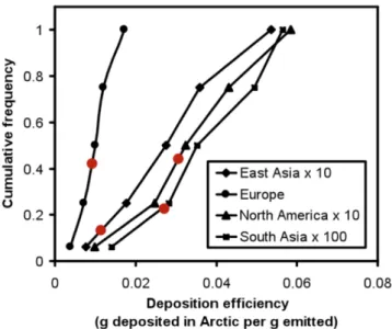
Fig. 9. Distribution of ensemble results for springtime Arctic de-position (March–April–May) (from Shindell et al., 2009), and com-parison of CAM results (red dots).
SFP. The ensemble adjustment for East Asia increases total SFP by only 2% and the change for South Asia is negligible. This transport may be a large uncertainty in Arctic radiative impact, but it is not a large uncertainty in global impact.
4.6 Total cryosphere forcing
Estimates of ice and snow forcing are more variable than those of atmospheric forcing. Koch et al. (2009)
summa-rized cryosphere forcing estimates, which range from +0.01 to +0.16 W m−2 and vary widely with the method of pa-rameterization and the reference value of emission. How-ever, some of these estimates use different emission rates and some are less physically based. Only one of the esti-mates is higher than +0.1 W m−2, and that value has been su-perceded. The lowest estimate comes from a model (GISS) that compared 1995 forcing with 1890. In addition, feed-backs make the response to cryosphere forcing highly uncer-tain. Cryosphere forcing in CAM is +0.037 W m−2from fos-sil fuel and biofuel, and +0.047 W m−2when open biomass burning is added (Flanner et al., 2009). Total fossil and biofuel emissions produce +0.06 W m−2 in GATOR-GCM (Abase,cry= 1.6; Jacobson, 2004; Jacobson, M. Z., personal communication, 2006) and +0.03 W m−2in the GISS model (Abase,cry= 0.8). We conclude that the CAM values used for cryospheric SFP are in the mid-range, but the uncer-tainties are about 100%. Sensitivity analyses by Flanner et al. (2007) give uncertainty as 60% due to three model assumptions, excluding emissions. We therefore choose a value of Acry,base= 1.0±0.6, which encompasses the two other physically-based model estimates.
4.7 Best estimates of SFP for BC and OM
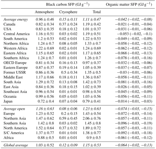
Table 1.Ensemble-adjusted Specific Forcing Pulse (SFP) for black carbon and organic matter. Uncertainties for OM are asymmetric and are presented as ranges.
Black carbon SFP (GJ g−1) Organic matter SFP (GJ g−1)
Atmosphere Cryosphere Total
Average energy 0.96±0.46 0.15±0.11 1.11±0.47 −0.042 (−0.02,−0.08)
Canada 0.82±0.34 0.37±0.24 1.19±0.42 −0.021 (−0.01,−0.04) USA 0.83±0.35 0.18±0.12 1.01±0.37 −0.031 (−0.01,−0.06) Central America 1.16±0.51 0.03±0.02 1.19±0.51 −0.053 (−0.02,−0.1) South America 1.2±0.53 0.02±0.01 1.22±0.53 −0.049 (−0.02,−0.09) Northern Africa 1.24±0.7 0.08±0.05 1.33±0.7 −0.058 (−0.02,−0.12) Western Africa 1.22±0.69 0.02±0.01 1.24±0.69 −0.062 (−0.02,−0.12) Eastern Africa 1.15±0.65 0.02±0.01 1.17±0.65 −0.068 (−0.02,−0.13) Southern Africa 1.24±0.7 0.01±0.01 1.26±0.7 −0.078 (−0.03,−0.16) OECD Europe 0.81±0.34 0.16±0.13 0.97±0.37 −0.032 (−0.02,−0.06) Eastern Europe 0.87±0.37 0.19±0.14 1.05±0.39 −0.037 (−0.02,−0.07) Former USSR 0.86±0.36 0.5±0.34 1.35±0.5 −0.03 (−0.01,−0.06) Middle East 1.17±0.66 0.18±0.11 1.36±0.67 −0.058 (−0.02,−0.11) South Asia 1.29±0.72 0.13±0.08 1.42±0.73 −0.081 (−0.03,−0.16) East Asia 0.84±0.36 0.18±0.15 1.02±0.39 −0.026 (−0.01,−0.05) Southeast Asia 0.96±0.54 0.01±0.01 0.98±0.54 −0.045 (−0.02,−0.09) Oceania 0.99±0.56 0.05±0.03 1.03±0.56 −0.056 (−0.02,−0.11) Japan 0.72±0.4 0.07±0.04 0.79±0.41 −0.014 (−0.01,−0.03)
Average open 1.16±0.63 0.08±0.06 1.23±0.63 −0.074 (−0.03,−0.15)
Europe 1.23±0.52 0.2±0.15 1.43±0.54 −0.072 (−0.03,−0.14) Northern Asia 1.47±0.62 0.59±0.45 2.06±0.76 −0.057 (−0.03,−0.11) Southern Asia 1.42±0.8 0.03±0.02 1.45±0.8 −0.096 (−0.03,−0.19) North America 1.52±0.64 0.37±0.32 1.89±0.72 −0.057 (−0.03,−0.11) S/C America 1.37±0.77 0.01±0.01 1.38±0.77 −0.092 (−0.03,−0.18) Africa 0.88±0.5 0.01±0.01 0.9±0.5 −0.061 (−0.02,−0.12)
Global average 1.03±0.52 0.12±0.09 1.15±0.53 −0.064 (−0.02,−0.13)
mixing adjustments yield large uncertainties in regional SFP even whenArgnis low. We weight regional SFP by emission rate to provide a global average SFPBCdir of 1.03±0.52 GJ/g.
For SFPBC
cry, we apply the baseline uncertainties discussed in Sect. 4.6 and uncertainties in Arctic deposition discussed in Sect. 4.5. Average cryosphere SFP is 0.12±0.09, al-though this varies greatly by region.
SFP for organic matter includes the baseline ensemble ad-justment (1.30 with an uncertainty range of [0.8, 2.2]) and the regional adjustments discussed in Sect. 4.4. As stated earlier, the asymmetric uncertainties are larger in the negative direc-tion.
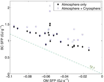
As SFPOM is negative, co-emissions of OM could offset positive forcing by BC. However, the magnitude of SFPBCdir is greater than that of SFPOMdir by about an order of magnitude. Figure 10 shows SFPBCdir plotted against SFPOMdir for each re-gion. The nearly linear relationship between the two is un-surprising, because our model had similar treatments of re-moval for both species. However, the good relationship does suggest that lifetime (τ ), more than varying forcing-per-mass (f ), is a dominant factor in determining SFP.
Relative emission rates of OM and BC differ by source, but the highest OM:BC ratio from a dominant source type is 12:1 for open burning of biomass (see emission rates given in Sect. 5). The ratio of SFPBCdir to SFPOCdir is greater than 12:1 for all regions, so the net effect of BC plus OM from that source is positive forcing. If only OM and BC were emit-ted, and direct plus cryosphere forcing were the only physi-cal effect, an OM:BC ratio of about 15:1 would result in zero or positive top-of-atmosphere direct forcing for any region. Any lower ratio has direct radiative warming, and the “neu-tral” ratio is greater for emissions in some regions. Values of SFPBCdir+cryare also shown in Fig. 10. Given the large un-certainties discussed earlier, there is still a significant proba-bility that some OM:BC ratios could result in cooling. This probability is lower when cryosphere forcing is significant.
Fig. 10.SFP for black carbon plotted versus SFP for organic matter for all 23 source-region combinations. A line which intercepts the origin and which has a slope of the OM:BC ratio from a particular source divides direct warming from direct cooling (above/below) by that source. The 12:1 line is given here because that OM:BC ratio is the highest of all the major sources. Therefore, central estimates for SFP indicate that the OM plus BC mix results in direct warming for all sources, although uncertainties are large.
4.8 Caveats
In our estimates of SFPTOA,dir+cry, we adjust a reference model (CAM) using an ensemble that incorporates multi-ple models. This procedure accounts for the possibility that CAM could be biased relative to other models. However, it does not address the fact that all models could be biased rel-ative to reality because of common, but incorrect, assump-tions about aerosol behavior. A quantitative assessment of the second possibility is greatly needed. To proceed further, the underlying causes of variation within models should be identified and evaluated with measurements, and models that more closely reproduce critical observations should be given a higher weighting.
Additional treatments are also needed to account for emerging knowledge about the properties and impacts of black carbon and organic matter. We incorporated adjust-ments for black carbon mixing and regional dependence of forcing because of the availability of multiple model results. For black carbon mixing, there is also general agreement on the physical nature of the enhancement. However, we did not apply the same treatment to many other possible effects. One example of an effect that needs to be addressed for black car-bon is enhanced forcing due to inclusions in cloud droplets (Jacobson, 2006). Examples for organic matter are absorp-tion due to some types of organic compounds (Kirchstetter et al., 2004) and the emerging understanding of organic aerosol hygroscopicity and particle growth (Jimenez et al., 2009).
5 Comparison of SFP with forcing and GWP values
While the main purpose of this paper is to present SFP for BC and OM, this measure has not previously appeared in the lit-erature. To compare the values provided here to earlier work, we translate SFP to forcing and Global Warming Potential, as discussed in Sect. 2. Globally-averaged measures are shown in Table 2 by emission-weighting regional SFP. Forcing and GWP for emissions from each region can be developed from Table 1 using the procedures outlined here.
5.1 Globally-averaged forcing
We calculate total aerosol forcing as emission rate times SFP. Estimates of year 2000 energy-related emissions by Bond et al. (2007), plus updated emission factors, are 4.8 Tg BC and 15 Tg OM. These values of OM include a source-dependent OM-to-OC ratio. The work presented earlier gives cen-tral values and uncertainties that are carried through SFP, the forcing per emission. Uncertainties in emission rates have been discussed extensively elsewhere (Bond et al., 2004), and we will not include them here. Multiplying the emission rates given above by the average SFP for energy-related emissions, converting units, and dividing by the area of the Earth gives +0.33±0.22 W m−2for BC (in-cluding cryosphere forcing) and−0.04 W m−2for OM, with an asymmetric uncertainty range of (−0.02,−0.08). Like-wise, we obtain forcing by multiplying SFP for open-burning emissions with average emission rates from van der Werf et al. (2006) (2.6 Tg BC and 30 Tg OM). For this source, we as-sume that organic matter is 1.4 times organic carbon for con-sistency with AeroCom emissions (Dentener et al., 2006). Forcing by open-burning emissions is is +0.20±0.08 W m−2 for BC, including cryosphere forcing, and −0.14 (−0.04, −0.27) W m−2 for OM, respectively. Table 2 summarizes these estimates and provides a breakdown between atmo-sphere and cryoatmo-sphere.
IPCC (Forster et al., 2007) reports anthropogenic forc-ing, or the difference between present-day and an atmo-sphere with 1750 emissions. The net anthropogenic emis-sions given by Dentener et al. (2006) are: 4.2 Tg BC and 10.7 Tg OC from energy-related combustion, and 2.1 Tg BC and 21.9 Tg OC from open burning. These emission rates yield anthropogenic forcing of +0.40±0.18 W m−2 for BC without cryosphere, +0.44±0.29 W m−2 for BC with cryosphere, and−0.13 (−0.05,−0.25) W m−2for OM.
Table 2. Global average forcing and global warming potentials derived from SFP combined with estimates of emissions (aerosol and anthropogenic forcing) or carbon dioxide forcing (global warming potentials). Uncertainties for OM are asymmetric and are presented as ranges.
BC TOA BC direct OM TOA direct
direct +cryosphere
Total aerosol forcing (W m2)
Global total 0.47±0.26 0.53± 0.30 −0.17 (−0.07,−0.35) Open biomass 0.19±0.07 0.20±0.08 −0.14 (−0.05,−0.27) Energy−related 0.28±0.19 0.33±0.22 −0.04 (−0.02,−0.08)
Anthropogenic forcing with IPCC−AR4 emissions (W m2)
Global total 0.40±0.18 0.44±0.29 −0.13 (−0.05,−0.25) Open biomass 0.15±0.06 0.16±0.13 −0.10 (−0.04,−0.20) Energy−related 0.25±0.12 0.29±0.16 −0.03 (−0.01,−0.06)
Global warming potential, 100-year
Global average 740±370 830±440 −46 (−18,−92)
Open biomass 830±330 880±370 −53 (−20,−100)
Energy−related 690±450 790±530 −30 (−12,−60)
Global warming potential, 20-year
Global average 2600±1300 2900±1500 −160 (−60,−320)
Open biomass 2900±1100 3100±1300 −180 (−70,−360)
Energy−related 2400±1600 2800±1800 −110 (−40,−210)
(+0.05 W m−2) is smaller than IPCC’s estimate because it includes new, more physically based studies.
5.2 Comparison with Global Warming Potential
Previously, measures of forcing-per-emission have been pre-sented as GWP values. For comparison, Table 2 shows GWPs calculated for 100-year and 20-year time horizons by dividing SFP by 1.4×10⁻³GJ g−1 and 4.0×10⁻⁴GJ g−1, respectively (see Sect. 2.5). In this discussion, we refer mainly to 100-year GWP values. The ratio of 100-year GWPs between two studies would be identical to the ratio of 20-year GWP values.
Compared with previous estimates of GWPBC by our group (Bond and Sun, 2005), the globally averaged value for direct forcing is similar but slightly higher (740±370 vs. 680). Uncertainties are about 50% of the total for BC. Direct GWPBCfor energy-related emissions (fossil fuel and biofuel) is somewhat lower than for open burning (690 vs. 830). Our atmospheric 100-year GWPBC from energy-related emis-sions is about 40% higher than the global mean average cal-culated by Reddy and Boucher (2007) and Fuglestvedt et al. (2009), who provided values of 480 and 460, respec-tively. The difference occurs largely because their models did not include internal mixing of black carbon with other aerosol components. As with direct forcing, addition of the cryosphere component increases globally-averaged GWP by
about 10%. This increase is regionally dependent, as can be inferred from Fig. 10.
Our value of GWPOM is−46 with an uncertainty range of (−18,−92). The average value for open burning (−53) is 80% greater than for energy-related combustion (−30) be-cause of seasonality. Fuglestvedt et al. (2009) used the same multi-model ensemble as we did, so their 100-year GWP for organic matter should be directly comparable. They provide a value of −69 for organic carbon; assuming that organic matter (which includes oxygen and hydrogen) is 1.4 times organic carbon by mass, their value becomes−49, very sim-ilar to ours.
6 Outlook, challenges, and caveats
In this paper, we compare modeled estimates for atmospheric and snow forcing of black and organic carbon, normalizing to emission rates. Our measure is a simple combination of model outputs, the Specific Forcing Pulse. It quantifies the impact per emission from a particular region, either for a global total or within a region, and can be easily translated to other policy-relevant measures. We recommend a method of combining model diversity with model improvements to provide best estimates.
The discussion throughout this paper has demonstrated that forcing values depend critically on emission rate for SLCFs. One should examine varying forcing estimates in light of the emission inventory used to obtain them, as that choice alone may account for large differences. For ex-ample, estimates of black carbon forcing for energy-related emissions alone have been compared with estimates for all emissions, and anthropogenic forcing (which excludes emis-sions in 1750) has been compared with total forcing. These variations reflect disagreement about source strength as well as model physics, and the sources of variation. Likewise, observationally-based estimates of forcing (e.g. Sato et al., 2003; Yu et al., 2006; Ramanathan and Carmichael, 2008) inherently include all emissions, not just those assumed in the model used. When observed and modeled forcing esti-mates differ, discrepancies could result from lifetime, nor-malized forcing, emissions, or some combination. Reducing uncertainties will require isolating the underlying reasons for disagreement and addressing them through focused measure-ments.
Because of continuing interest in SLCFs and their mitiga-tion, model estimates of total, sectoral or individual-source forcing are becoming common. To place new estimates in context of others’ work, individual model results should al-ways be accompanied by a comparison with model ensem-bles. Such comparisons should use normalized values, such as SFP, normalized forcing, or lifetime.
The SFP presented here incorporates model estimates of atmospheric and snow forcing. Future analysis should focus on two improvements:
Cloud changes. Changes in aerosol emissions also cause differences in cloud albedo (“first indirect”), cloud lifetime (“second indirect”), and cloud amount due to atmospheric heating (“semi-direct”). Such changes often result in nega-tive forcing (Chen et al., 2010; Koch and DelGenio, 2010), which would reduce the magnitude of the SFP for black car-bon, and make that of organic carbon even more negative. There is a dearth of model studies examining cloud responses to emission changes, rather than total impacts. Such studies are needed before any measure can incorporate these impor-tant effects.
Incorporating observations. The possibility that all mod-els could be incorrect is a serious one. Observational con-straints and uncertainties should be embedded in the SFP.
Not present in our discussion is a recent model estimate of very high atmospheric forcing by black carbon (Ramanathan and Carmichael, 2008). Their reported total forcing of +0.9 W m−2 is higher than many other modeled estimates. However, because the estimate was partly based on observa-tions, the large observed forcing could also result from actual emissions being higher than modeled emissions. Until the exact causes of difference are isolated, such estimates cannot be used to provide an “impact-per-emission” measure like the SFP. However, the great difference from modeled values should serve as a caution that emissions, model processes, or both contain uncertainties that are not fully reflected in global simulations.
Appendix A
Quantifying immediate radiative forcing by black carbon and organic matter with the Specific Forcing Pulse
Although global chemical-transport models usually do not use pulse emission functions, SFP can be determined from their output, with some limitations. In this section, we demonstrate why this is so using the simple box model shown in Figure A1. In this box, a first-order process with rate con-stant 1/τS is responsible for all removal. The solution to the first-order differential equation describing the concentra-tion has a familiar exponential form. After an emission pulse of magnitudeM0S into the box, the integrated concentration from zero to infinity isτSM0S. This integrated concentration is equivalent to the integral of burden (bS)over surface area and time in Equation 1. If the mass that remains in the box captures energy per time per massfS,, the integrated energy for a box is (τS fSM0S), and the added energy per emitted mass is (τS fS). This would be the calculated SFP for the material in the box model. A positive sign indicates net en-ergy capture, retention, or increase; a negative sign indicates energy rejection, which may occur either by reflection of en-ergy or increased re-emission. In the same box at steady state with a continuous emission rateM¯S(g s−1), the steady-state concentration is (τSM¯S)and the rate of energy addition (or loss) is given by (τSfSM¯S). The latter is commonly called forcing, and the forcing per mass is (τSfS), which also hap-pens to be SFP. Figure A1b illustrates some of the relation-ships betweenτSfS (or SFP) and more commonly reported measures such as column burdenbS, emission rateM¯S, and
total forcing.
1522 T. C. Bond et al.: Immediate radiative forcing by black carbon and organic matter τ
τ
τ
Fig. A1. (a)Simple box model demonstrating factors that govern impacts on energy balance due to addition of a speciesS. Net energy addition per mass (fS) is shown by green arrows indicating incoming and reflected solar radiation, and red arrows indicating absorption and dissipation as heat. Other interactions with radiation (e.g. re-emission of infrared energy, absorption by the species on the Earth’s surface) can be framed in similar terms but are not presented here. First-order removal has rate constant 1/S (inverse of lifetime). (b)Calculation flow for box in steady state, with blue “x” indicating multiplication (e.g., total burden = lifetime multiplied by emission rate). Energy added (Specific Forcing Pulse) does not depend on emission rate.
achieve steady-state conditions for a pollutant with a lifetime of 9 years. Thus, even if we chose to apply the SFP concept to methane, using global models to determine its value would require multi-decade simulations.
Of course, in the Earth system, τS, fS, and emission rate all vary in space and time. SFP derived from mod-eled forcing-to-emission ratios could depend on the emis-sion spatial and temporal distributions used in the model, among other factors. Annually-averaged concentrations and forcing from chemical-transport models can provide average values of SFP, but the same model experiments cannot iso-late seasonally-dependent values of SFP. Instantaneous val-ues offScan be derived from the ratio between total forcing and column burden at any time during the simulation. How-ever,τS(the other component of SFP) cannot be obtained by dividing instantaneous values of burden and emission rate. Nevertheless, values ofτSandfScan aid in diagnosing rea-sons for differences in SFP between searea-sons or regions.
Appendix B
SFP and temperature change
Locations of SLCF concentrations and forcing depend upon the emitting region (Berntsen et al., 2006). Furthermore, gional forcing is not proportional to regional temperature re-sponse. As a first step in representing this complex situation, we propose the following equation:
Ik(t )=
Z τ
0
J
X
j=1
Rk,j·γjS I
X
i=1
SFPS j,i·ei(t )
!
dt (B1)
where SFPSj,iis the forcing in regionj due to an emission of S in regioni,γjS is the ratio between effective forcing and radiative forcing and accounts for the “fast response” (Shine et al., 2003; Forster and Taylor, 2006; Lohmann et al., 2010) to speciesSin regionj, andRk,jS is the response in regionk to a CO2-like forcing in regionj after timet. The termγS encompasses some, but not all, of the effects that are tradi-tionally called “efficacy” or “efficiency.”
In matrix form, I=
Z τ
0
R(t )·γS·SFPS·eS(t )dt (B2) whereI is a vector in which thek-th element represents im-pact in regionk, andeis a vector in which thei-th element represents emission in regioni. SFPis a matrix for which thej-th row and i-th column represent forcing in regionj due to emission in regioni; γ is a diagonal matrix; andR
is a matrix for which thek-th row andj-th column give the response (temperature response or other chosen change) to forcing in regionj. We note that the “regions” in the equa-tion could be smaller than the large regions presented in this paper, even as small as a city. However, uncertainties in at-mospheric transport and impact may preclude such detailed estimates of SFP.