Improved sea level record over the satellite altimetry era (1993–2010) from the Climate Change Initiative Project

(1)

OSD

11, 2029–2071, 2014

Improved sea level record over the satellite altimetry era

M. Ablain et al.

Title Page

Abstract Introduction

Conclusions References

Tables Figures

◭ ◮

Back Close

Full Screen / Esc

Printer-friendly Version Interactive Discussion

Discussion

P

a

per

|

Discus

sion

P

a

per

|

Discussion

P

a

per

|

Discussion

P

a

per

|

Ocean Sci. Discuss., 11, 2029–2071, 2014 www.ocean-sci-discuss.net/11/2029/2014/ doi:10.5194/osd-11-2029-2014

This discussion paper is/has been under review for the journal Ocean Science (OS). Please refer to the corresponding final paper in OS if available.

Improved sea level record over the

satellite altimetry era (1993–2010) from

the Climate Change Initiative Project

M. Ablain1, A. Cazenave2, G. Larnicol1, M. Balmaseda11, P. Cipollini7,

Y. Faugère1, M. J. Fernandes10,14, O. Henry2, J. A. Johannessen3, P. Knudsen6, O. Andersen6, J. Legeais1, B. Meyssignac2, M. Picot12, M. Roca8, S. Rudenko9,

M. G. Schar_ffenberg4, D. Stammer4, G. Timms5, and J. Benveniste13

1

Collecte Localisation Satellite(CLS), Ramoville Saint-Agne, France

2

Laboratoire d’Etudes en Géophysique et Océanographie Spatiales (LEGOS), Toulouse, France

3

Nansen Environmental and Remote Sensing Center (NERSC), Bergen, Norway

4

University of Hamburg, Hamburg, Germany

5

CGI, London, UK

6

Technical University of Denmark (DTU), Lyngby, Denmark

7

National Oceanography Centre (NOC), Southampton, UK

8

isardSAT, Barcelona, Catalunya, Spain

9

(2)

OSD

11, 2029–2071, 2014

M. Ablain et al.

Title Page

Tables Figures

◭ ◮

Back Close

Full Screen / Esc

Discussion

P

a

per

|

Discus

sion

P

a

per

|

Discussion

P

a

per

|

Discussion

P

a

per

10

Faculdade de Ciências, Universidade do Porto, 4169-007 Porto, Portugal

11

European Centre for Medium-Range Weather Forecasts (ECMWF), Reading, UK

12

Centre National d’Etudes Spatiales (CNES), Toulouse, France

13

European Space Agancy (ESA), ESRIN, Frascati, Italy

14

Centro Interdisciplinar de Investigação Marinha e Ambiental (CIIMAR/CIMAR), Universidade do Porto, 4050-123 Porto, Portugal

Received: 7 July 2014 – Accepted: 16 July 2014 – Published: 21 August 2014

Correspondence to: M. Ablain ([email protected])

(3)

OSD

11, 2029–2071, 2014

M. Ablain et al.

Title Page

Tables Figures

◭ ◮

Back Close

Full Screen / Esc

Discussion

P

a

per

|

Discus

sion

P

a

per

|

Discussion

P

a

per

|

Discussion

P

a

per

|

Abstract

Sea level is one of the 50 Essential Climate Variables (ECVs) listed by the Global Cli-mate Observing System (GCOS) in cliCli-mate change monitoring. In the last two decades, sea level has been routinely measured from space using satellite altimetry techniques. In order to address a number of important scientific questions such as: “Is sea level 5

rise accelerating?”, “Can we close the sea level budget?”, “What are the causes of the regional and interannual variability?”, “Can we already detect the anthropogenic forc-ing signature and separate it from the internal/natural climate variability?”, and “What are the coastal impacts of sea level rise?”, the accuracy of altimetry-based sea level records at global and regional scales needs to be significantly improved. For example, 10

the global mean and regional sea level trend uncertainty should become better than 0.3 and 0.5 mm year−1, respectively (currently of 0.6 and 1–2 mm year−1). Similarly, interannual global mean sea level variations (currently uncertain to 2–3 mm) need to be monitored with better accuracy. In this paper, we present various respective data improvements achieved within the European Space Agency (ESA) Climate Change 15

Initiative (ESA CCI) project on “Sea Level” during its first phase (2010–2013), using multi-mission satellite altimetry data over the 1993–2010 time span. In a first step, using a new processing system with dedicated algorithms and adapted data process-ing strategies, an improved set of sea level products has been produced. The main improvements include: reduction of orbit errors and wet/dry atmospheric correction er-20

rors, reduction of instrumental drifts and bias, inter-calibration biases, intercalibration between missions and combination of the different sea level data sets, and an improve-ment of the reference mean sea surface. We also present preliminary independent vali-dations of the SL_cci products, based on tide gauges comparison and sea level budget closure approach, as well as comparisons with ocean re-analyses and climate model 25

(4)

OSD

11, 2029–2071, 2014

M. Ablain et al.

Title Page

Tables Figures

◭ ◮

Back Close

Full Screen / Esc

Discussion

P

a

per

|

Discus

sion

P

a

per

|

Discussion

P

a

per

|

Discussion

P

a

per

1 Introduction

Global warming in response to the anthropogenic green-house gases emissions has already shown several visible consequences, among them the increase of the Earth’s mean air temperature and ocean heat content, melting of glaciers, and loss of ice masses from glaciers and the Greenland and Antarctica ice sheets. Ocean warming 5

and land ice melting in turn are causing sea level to rise, with potentially negative im-pacts in many low-lying regions of the world. The precise measurement of sea level changes as well as its di_fferent components, at global and regional scales, is an impor-tant issue for a number of reasons. It provides information on how the climate system

and its different components respond to global warming and on the relative

contribu-10

tions of anthropogenic forcing and natural/internal climate variability. This also allows validating the climate models developed for projecting future changes as the models are supposed to correctly reproduce present-day and recent-past changes. The Global Climate Observing System (GCOS) has recently defined a set of 50 climate variables (called Essential Climate Variables – ECVs) that need to be precisely monitored on 15

the long-term in order to improve our understanding of the climate system, its function-ing and its response to anthropogenic forcfunction-ing, as well as to provide constraints for cli-mate modelling (GCOS, 2011). In 2010, the European Space Agency (ESA) developed a new program, the Climate Change Initiative (CCI), dedicated to reprocessing a set of 13 ECVs currently observed from space; among them, the satellite altimetry-based sea 20

level ECV. The objective of the CCI sea level project (called SL_cci below) was to pro-duce a consistent and precise sea level record covering the last two decades, based on the reprocessing of all satellite altimetry data available from all missions (including the ERS-1&2 and Envisat missions, in addition to the TOPEX/Poseidon, Jason-1&2 and Geosat Follow-on (GFO) missions). During the 1st phase of the project, that lasted 25

(5)

OSD

11, 2029–2071, 2014

M. Ablain et al.

Title Page

Tables Figures

◭ ◮

Back Close

Full Screen / Esc

Discussion

P

a

per

|

Discus

sion

P

a

per

|

Discussion

P

a

per

|

Discussion

P

a

per

|

geophysical corrections adapted to each satellite mission have been implemented af-ter being evaluated and selected. Other improvements concern the reduction of instru-mental drifts and biases (in particular for the Envisat mission), a new calculation of the mean sea surface used as reference, the method used for geographical averag-ing of sea surface height data and the reduction of systematic bias between missions. 5

The main SL_cci products computed during the phase 1 consist of: (1) a Global Mean Sea Level (GMSL) time series at monthly interval between January 1993 and Decem-ber 2010, and (2) a global gridded sea level time series (resolution 0.25◦

×0.25◦) at the same time interval.

This paper thus intends to provide a global overview of the main results obtained in 10

the frame of the SL_cci project. We firstly describe the validation protocol (Sect. 2) that has been applied to evaluate and select the algorithms and corrections used (Sect. 3) to generate the SL_cci products (described in Sect. 4). Then, Sect. 5 and 6 are focused on the assessment and the error characterization.

2 Definition of a formal validation protocol of validation

15

The altimetry data processing system used to compute sea level (or the Sea Sur-face Height/SSH) integrates a number of components: the altimeter range measure-ment (Range), the satellite orbit height (Orbit) and the instrumeasure-mental and geophysical corrections. The estimation of these components needs additional information

com-ing from di_fferent domains as orbitography (a force model) for the precise orbit

de-20

termination, geodesy (geoid, mean sea surface, global isostatic adjustment (GIA), etc.), atmosphere (pressure, wind, dry and wet troposphere, etc.), and ocean (ocean tides, sea state, etc.). This information may be eventually linked together either di-rectly or indidi-rectly. Because of these complex interactions, sea level estimates (i.e.,

SSH ₌ Orbit RangePN

i=0

(6)

OSD

11, 2029–2071, 2014

M. Ablain et al.

Title Page

Tables Figures

◭ ◮

Back Close

Full Screen / Esc

Discussion

P

a

per

|

Discus

sion

P

a

per

|

Discussion

P

a

per

|

Discussion

P

a

per

an optimized sea level calculation requires a large number of algorithms and correc-tions that need to be rigorously validated and regularly updated.

In the framework of the SL_cci project, we developed a new formal validation protocol which allowed us to evaluate the impact of new altimeter corrections or standards on a sea level record of climate quality, i.e., precise enough for climate studies. It consists 5

in comparing the new altimeter corrections with corrections designed as a reference through their impact on the sea level calculation. This was done using a common set of validation diagnoses defined in such a way that they fulfil the sea level accuracy and precision requirements. The validation diagnoses are distributed into 3 distinct families allowing the assessment of altimetry data with complementary objectives:

10

1. the “global internal analyses” with the aim of checking the internal consistency of a specific mission related-altimetry system by analyzing the computed sea level, its instrumental parameters (from altimeter and radiometer) and associated geo-physical corrections,

2. the “global multi-mission comparisons” allowing evaluation of the coherence be-15

tween two different altimetry systems through comparison of SSH data,

3. the “altimetry-in-situ data comparison” dedicated to the computation of the sea level di_fferences between altimeter data and in-situ sea level measurements; e.g., from tide gauges or Argo-based steric sea level data (Valladeau et al., 2012); this 3rd approach allows for the detection of potential drifts or jumps in the long-term 20

sea level time series.

For each family, several validation diagnoses have been defined using elementary statistical approaches (e.g., mean, standard deviation, linear regression) and data rep-resentation (e.g., global mean time series, maps, histograms, periodograms, etc.). Other tests based on altimeter correction differences, sea surface height differences 25

(7)

OSD

11, 2029–2071, 2014

M. Ablain et al.

Title Page

Tables Figures

◭ ◮

Back Close

Full Screen / Esc

Discussion

P

a

per

|

Discus

sion

P

a

per

|

Discussion

P

a

per

|

Discussion

P

a

per

|

Plan (PVP) report of the SL_cci project (see appendix for all referenced SL_cci reports available on the SL_cci website).

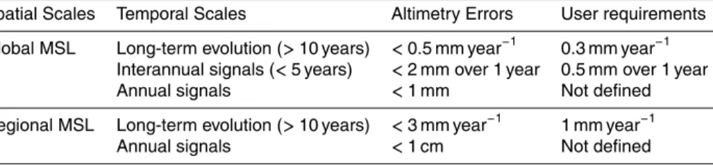
The analyses of these diagnoses were performed for different spatial (global mean

and regional sea level, mesoscale) and temporal scales (Table 1, left panel): long term

>10 years, interannual 2–5 years, and periodic signals-annual, semi-annual scales.

5

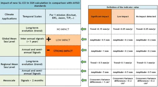
These spatio-temporal scales were chosen according to the sea level user require-ments document (SL_cci User Requirerequire-ments Document, 2010) presented in the last section. This formal validation protocol allows us to determine, for each spatial and tem-poral scale, the level of impact (i.e. low or strong) of the new altimetry corrections on the sea level calculation (Table 1, right panel). For instance, if a new altimetry correction 10

causes a GMSL trend>0.15 mm year−1 _{(over a period} _>_{10 years), we consider that}

the impact is strong, whereas if the trend effect is in the range 0.05–0.15 mm year−1, it is assumed low, and negligible below 0.05 mm year−1.

Our goal is also to check whether the new altimeter corrections improved or degraded the sea level estimates for each time scale. In general, it was possible to clearly de-15

tect either improvement or degradation (illustrated Table 1, left panel, with the symbols

“₊” or “−” meaning improvement or degradation). For example, increased consistency

between GMSL trends derived from two di_fferent altimetry missions or from in-situ mea-surements suggests that the accuracy/precision of sea level data has been improved. In only a few cases, the diagnoses were inconclusive. This occurred when errors of al-20

timetry missions are of the same order of magnitude or correlated (e.g. same error for the regional mean sea level trends). In these rare cases, thorough investigations could be conducted through a “case by case” approach. When no obvious conclusion could be reached, the sea level di_fferences due to the new correction were then allocated to the altimetry error budget (see Sect. 6).

25

(8)

OSD

11, 2029–2071, 2014

M. Ablain et al.

Title Page

Tables Figures

◭ ◮

Back Close

Full Screen / Esc

Discussion

P

a

per

|

Discus

sion

P

a

per

|

Discussion

P

a

per

|

Discussion

P

a

per

quickly relevant information about the impact of each correction on the sea level prod-ucts.

3 Development, validation and selection of new altimeter corrections

and algorithms

In this section, we present applications of the formal validation protocol described in 5

Sect. 2. An important output of the SL_cci project was the development of new altimetry corrections (mentioned in Sect. 2) and algorithms (e.g. for merging data from different altimetry missions). A total of 42 new corrections/algorithms were evaluated within the project using the validation protocol described above. The reference standards were those used for AVIS0 products (Dibarboure et al., 2011) at the beginning of the SL_cci 10

project.

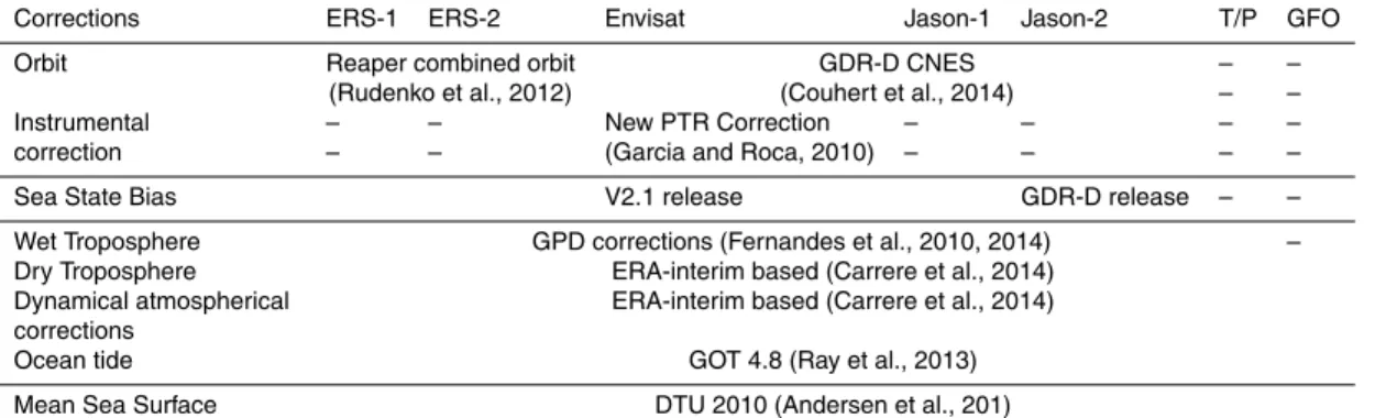
Table 1 presents the selected corrections for each component and altimetry missions (for detailed information, see “SL_cci Validation Report, Executive Summary”, 2013).

One of the most dramatic improvements comes from the use of ERA-interim reanaly-ses (from the European Centre for Medium-Range Weather Forecasts (ECMWF); Dee 15

et al., 2011) instead of operational ECMWF fields to calculate the dry tropospheric and other dynamical atmospheric corrections. Applying our validation protocol, we noted strong improvements at mesoscale and regional spatial scales, over the first altimetry decade (1993–2003) (Carrere et al., 2014; “SL_cci Validation reports, Atmospheric cor-rections”). The GMSL error reduction (Table 2, top) obtained from crossover analyses 20

is of the order of 2.5 cm on the early years of altimetry era (1993–1995). Then, the error decreases linearly until 2004, and remains stable close to 0, during recent years. The improvement observed in the first decade (1993–2003) is stronger at high latitudes (6 cm) where the atmospheric pressure and wind fields have strong high frequency variability. Looking at regional sea level trends (Table 2), significant trend differences 25

(9)

OSD

11, 2029–2071, 2014

M. Ablain et al.

Title Page

Tables Figures

◭ ◮

Back Close

Full Screen / Esc

Discussion

P

a

per

|

Discus

sion

P

a

per

|

Discussion

P

a

per

|

Discussion

P

a

per

|

Similarly, the model-based wet tropospheric correction was also strongly improved (until 1 cm error reduction on the GMSL) before 2002 using ERA-interim instead of ECMWF operational fields (Legeais et al., 2014). While not as good as the wet tro-posphere corrections derived from the on-board microwave radiometers (MWR), the ERA-Interim wet tropospheric correction allows us to better characterise the uncer-5

tainty of wet troposphere content over the long term (Thao et al., 2014; Legeais et al., 2014). However, this was not used in the sea level calculation where the radiometer-based corrections were preferred.

In parallel, the radiometer-based corrections have been improved using combined estimates from valid on-board MWR values, Global Navigation Satellite Systems 10

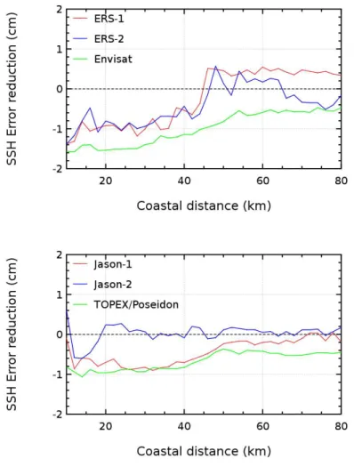
(GNSS) measurements and ECMWF model (ERA Interim fields) in areas where the MWR measurements are degraded due to, e.g., land or ice contamination or instrument malfunction (Fernandes et al., 2010, 2014). This new correction, called GNSS-derived Path Delay (GPD), computed for all ESA and reference missions, brings improvements mainly in coastal areas and in the polar regions. In Fig. 3, the sea level error reduction 15

is plotted vs. the distance to the coast using the new GPD corrections instead of the reference radiometer-based corrections. For almost all missions, except Jason-2 which already benefits from an improved coastal radiometer correction (Brown et al., 2009), there is a significant SSH error reduction, close to 1 cm between 20 and 40–50 km from the coast. Improvements have also been noticed in the open ocean, especially 20

for TOPEX data (Fernandes et al., 2014) where radiometer data gaps degrade the in-terpolation process. Finally, the GPD corrections have been selected for all altimeter missions because of the noted improvement in the sea level calculation at short and long time scales, mainly in coastal and polar regions.

Orbit error is the main source of the error for the long-term sea level evolution at 25

oceanic basin scales (Couhert et al., 2014). Strong e_fforts have been made within

(10)

OSD

11, 2029–2071, 2014

M. Ablain et al.

Title Page

Tables Figures

◭ ◮

Back Close

Full Screen / Esc

Discussion

P

a

per

|

Discus

sion

P

a

per

|

Discussion

P

a

per

|

Discussion

P

a

per

model used in the orbit computation are crucial as far as the quality of orbit solutions is concerned. After analyzing all orbit solutions for all the missions, the REAPER com-bined orbit solutions (Rudenko et al., 2012) have been selected for ERS-1 and ERS-2, with the new CNES GDR-D orbit solutions (Couhert et al., 2014) being selected for

the Jason-1, Jason-2 and Envisat missions. Strong e_ffects were observed on the

re-5

gional sea level trend, in the range of 1–2 mm year−1, with large patterns at hemispheric scale when using static and time variable Earth gravity field models for orbit computa-tion (Fig. 4). Thanks to cross-comparisons between altimetry missions (Ollivier et al., 2012) and with in-situ measurements (Valladeau et al., 2012), we have demonstrated that these new orbit solutions dramatically improved the regional sea level trends. Fur-10

thermore, this inter-comparison, using di_fferent orbit solutions, provided interesting in-formation on the orbit sensitivity to the choice of the Earth gravity field model (Rudenko et al., 2014).

In addition to these major improvements, other corrections were also selected, al-though their impact on the sea level estimate was lower. These concern the iono-15

spheric correction with the use of the NIC09 (New Ionosphere Climatology) model for ERS-1 (Scharroo et al., 2010), the GOT4.8 (Geocentric Ocean Tide) ocean tide solu-tion (Ray et al., 2013) and the DTU10 (Danish Technical University) mean sea surface (Andersen et al., 2010) for all missions. In addition, we also benefited from the repro-cessing of Envisat and Jason-2 level-2 products “GDR V2.1” (Ollivier et al., 2012) and 20

“GDR-D” (Philipps et al., 2013). This allowed us to increase the data coverage (mainly for Envisat) and to improve the sea-state bias corrections along with instrumental bias and drift corrections. For the latter, the impact is strong for Envisat since a global

instru-mental drift of about 2 mm year−1 _{was identified and corrected in the altimeter range}

(Thibaut et al., 2010; Roca and Thibaut, 2009; Garcia and Roca, 2010). It is worth 25

mentioning that the SL_cci project contributed to correct this anomaly, while Envisat was not designed for climate studies but rather mesoscale variability.

(11)

OSD

11, 2029–2071, 2014

M. Ablain et al.

Title Page

Tables Figures

◭ ◮

Back Close

Full Screen / Esc

Discussion

P

a

per

|

Discus

sion

P

a

per

|

Discussion

P

a

per

|

Discussion

P

a

per

|

the verification phase between these missions, systematic geographical biases could be detected. These biases are mainly latitude-dependent, with variations close to 0.5 cm between Jason-1 and Jason-2, and 1 cm between TOPEX and Jason-1. Cor-recting these regional and systematic sea level differences (see the SL_cci Validation Report, Regional SSH bias corrections between altimetry missions, 2012), led us to 5

better combine together these 3 altimetry missions and therefore better estimate the long-term sea level evolution at regional scales. The impact of these corrections on

regional MSL trends plotted in Fig. 5 from 1993 to 2010 is close to_±0.3 mm year−1_,

with large hemispheric dependence.

4 New CCI-based sea level records

10

Sea level products were generated using the new altimeter corrections described in Sect. 3. The same procedure was adopted as for the SSALTO DUACS (Segment Sol Multimission Altimetrie et Orbitographie, Data Unification and Altimeter Combination System) system (Dibarboure et al., 2011). After calculating the along-track sea level for each of the 7 missions (TOPEX/Poseidon, Jason-1, Jason-2, ERS-1, ERS-2, En-15

visat and Geosat Follow-on) over the [1993, 2010] period, the main steps consisted of: combining all missions together, reducing the orbit and the long wavelength er-rors, computing the gridded sea level anomalies using an objective analysis approach (Ducet et al., 2000; Le Traon et al., 2003), and generating mean sea level products (e.g., GMSL time series, gridded sea level time series, etc.) dedicated for climate stud-20

ies. The SL_cci products are monthly grids time series with a spatial resolution of 0.25◦ degrees using a rectangular projection. The GMSL time series (also at monthly inter-val) is based on the geographical averaging over the oceanic domain observed by the altimetry data (82◦_{S to 82}◦_{N) of the gridded data. Additional products (called}

indica-tors) are provided, e.g., GMSL trend, regional MSL trends, amplitudes and phases of 25

(12)

OSD

11, 2029–2071, 2014

M. Ablain et al.

Title Page

Tables Figures

◭ ◮

Back Close

Full Screen / Esc

Discussion

P

a

per

|

Discus

sion

P

a

per

|

Discussion

P

a

per

|

Discussion

P

a

per

Access to the SL_cci products can be obtained by sending an email at the follow-ing address: [email protected]. The Product User Guide (PUG, 2013) and Product Specification Document (PSD, 2013) provide further details.

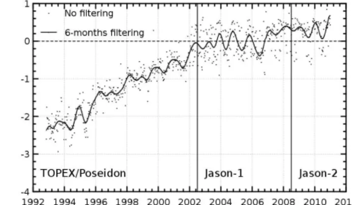
Comparisons between the SL_cci product and the AVISO-2010 products (Dibarboure et al., 2011) were performed by applying the formal validation protocol 5

described above (Sect. 2). Concerning the GMSL trend, similar values were obtained

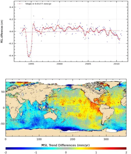
for both time series: 3.2 mm year−1over the 1993–2010 time span. At the interannual

time scale, (highlighted by calculating the di_fference between the two GMSL time

se-ries (Fig. 6, top panel), small differences in the range 1–2 mm or lower are noticed,

except for 1994 where a 4 mm jump is observed. This jump is due to an anomalous 10

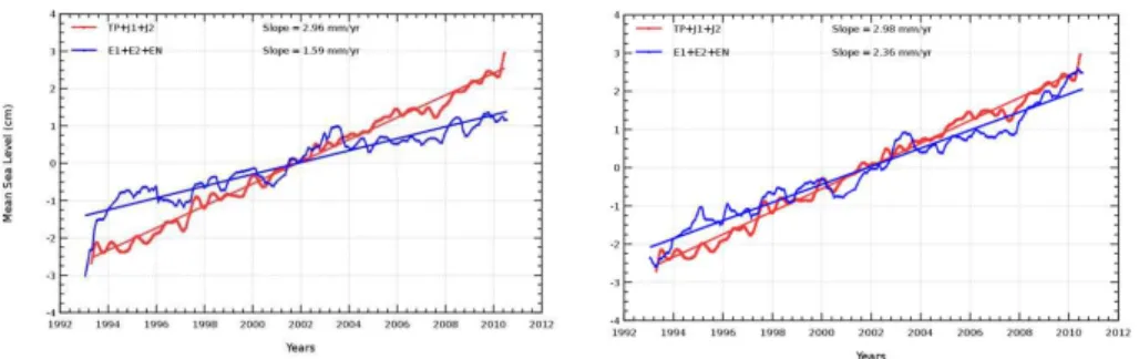
value of the AVISO-2010 products caused by an inadequate merging of the TOPEX data with the ERS-1 data of the non-repetitive geodetic phase (Pujol et al., 2014). The most impressive result is obtained by separating the ERS-1/ERS-2/Envisat and TOPEX/Jason-1/Jason-2 global GMSL time series using alternately the old and new al-timeter corrections (Fig. 7): the trend di_fference between both time series is now close 15

to 0.6 mm year−1 from 1993 to 2010 instead of about 1.5 mm year−1 previously. This

improved consistency does not have a direct impact on the GMSL trend, which only depends on the TOPEX/Jason-1/Jason-2 missions. However, this provides increased confidence in the long-term GMSL time series.

Looking at the regional sea level trend di_fferences (Fig. 6, bottom panel), large geo-20

graphically correlated structures are observed. Their amplitude is in the_±2 mm year−1

range. They primarily result from the new orbit solutions (hemispheric effects), the new ERA-interim atmospheric fields (at high latitudes), the new wet tropospheric correction, and the geographical biases arising when linking altimetry missions together. Compar-ing with in-situ measurements (tide gauges and Argo-based steric sea level) indicates 25

(13)

OSD

11, 2029–2071, 2014

M. Ablain et al.

Title Page

Tables Figures

◭ ◮

Back Close

Full Screen / Esc

Discussion

P

a

per

|

Discus

sion

P

a

per

|

Discussion

P

a

per

|

Discussion

P

a

per

|

method between the in-situ and altimetry data is larger than the target signal (Couhert et al., 2014). We also examined the periodic (annual and semi-annual) sea level

sig-nals. We found differences in the order of 5 mm on average for the amplitude of the

annual signal. In some regions (the tropics), the differences can reach 1 cm. Whilst we think that the new seasonal signal is improved compared to the AVISO-2010 products, 5

it is not possible to demonstrate this through any independent validation diagnoses. In-deed, comparisons with the in-situ measurements are not accurate enough to observe such signals.

5 Validation of the temporal and spatial variations of global sea level:

The SL_cci products delivered at the end of Phase 1 are currently under validation and 10

evaluation. Two di_fferent approaches have been developed:

1. Assessment of the accuracy of the SL_cci products through their use in ocean reanalyses and Earth system models

2. Assessment of the global sea level budget

In approach (1), the accuracy of the SL_cci data is evaluated by quantifying the 15

model performances and robustness (compared to the use of using a reference sea level data set, e.g., AVISO standard data) in representing a number of physical pro-cesses (e.g., the sea level drop associated with the 2011 La Niña, the Indonesian

through flow, changes in the Arctic circulation, effects of monsoon on sea level,

re-gional sea level fingerprint due to wind stress, steric sea level trend patterns, etc.). 20

(14)

OSD

11, 2029–2071, 2014

M. Ablain et al.

Title Page

Tables Figures

◭ ◮

Back Close

Full Screen / Esc

Discussion

P

a

per

|

Discus

sion

P

a

per

|

Discussion

P

a

per

|

Discussion

P

a

per

5.1 Assessment based on numerical ocean models

Ocean model simulations are an e_ffective way of translating wind and heat fluxes

in-formation into sea level variations, thus providing independent verification of their con-tribution to sea level. Sea level from ocean-only simulations at di_fferent resolutions (1◦ _{degree, 1}_/₄◦ _{of degree) has been contrasted with along-track data and with}

grid-5

ded (filtered and merged) sea level maps from AVISO (Dibarboure et al., 2011) and SL_cci. The statistics of the comparison (correlation, rms error, differences in trends)

were similar when using AVISO and SL_cci data. Di_fferences between models and any

observed estimations were much larger than the differences between observational

products. The spatial patterns of these differences were suggestive of model error. For 10

instance, small scale sea level variability is much larger in observed products than in models, which is consistent with insufficient resolution in the models. In contrast the low frequency and large scale variability is more obvious better resolved in models. The large scale patterns of interannual variability and trends are consistent between models and observations, but differences exist associated with the precise location of 15

strong current systems, which models struggle to capture. This information is in itself interesting, and suggests that a large part of the sea level variability is of dynamic na-ture, associated with changes in the wind-driven circulation. Both AVISO and SL_cci were useful to detect improvements in ocean model simulations due to the increased resolution.

20

In the Arctic Ocean the SL_cci reprocessed data reveals some distinct features of the elevated trend in sea level rise, notably: in the Beaufort Sea, in the Norwegian Sea, in the Sub-Polar gyre, and in the North East Atlantic south of the Iceland-Faroe

ridge. The Beaufort Sea rise of about 6.5–7 mm year−1 has also been reported by

Morison et al. (2011) and Laxon et al. (2012), while the elevated feature of around 6– 25

7 mm year−1_{, as detected in the SL_cci field in the Lofoten Basin of the Norwegian Sea,}

(15)

OSD

11, 2029–2071, 2014

M. Ablain et al.

Title Page

Tables Figures

◭ ◮

Back Close

Full Screen / Esc

Discussion

P

a

per

|

Discus

sion

P

a

per

|

Discussion

P

a

per

|

Discussion

P

a

per

|

A first look at the three GCMs (General Circulation Model), NorESM (Norwegian Earth System Model), Hadley and IPSL (Institut Pierre-Simon Laplace), reveals large individual differences in the trend of sea level change, both regarding the overall trend as well as in its regional characteristic changes. In comparison to the SL_cci sea level

change the NorESM simulations (1◦ _{resolution) yield the best agreement both in the}

5

Sub-Polar gyre, in the northeast Atlantic Ocean south of the Iceland-Faroe ridge, in the Lofoten basin of the Norwegian Sea and in the Beaufort Gyre. This intercomparison of the SL_cci trends with the trends derived from the three GCMs is interesting and can provide evidence for how realistic the model simulations are with respect to the variability of the water masses (steric height contribution) and variability, spreading 10

and accumulation of freshwater discharges from melting ice sheets and glaciers (mass changes).

In summary, as it was to be expected from the beginning, even ocean-only simula-tions are not able to identify the incremental improvement of SL_cci vs. its predecessor. Nevertheless, this validation exercise has shown that the SL_cci is a robust dataset for 15

ocean and climate models validation, and can discern verification metrics.

5.2 Assessment based on ocean data assimilation

Data assimilation methods can be very e_ffective methods to test the quality of the input data. This approach was used here to evaluate the SL_cci products, either by direct as-similation of the product (active mode) or by simple comparison with a reference state 20

(passive mode), obtained by a forced ocean-model combined with in-situ observations, and even other sea level observations. In this way, the reference state, containing in-formation both from model (winds) and in-situ observations, should have less error than an ocean-model simulation. The passive comparison can be done a-posteriori (by comparing and ocean reanalyses with SL_cci), or during the assimilation process, 25

(16)

OSD

11, 2029–2071, 2014

M. Ablain et al.

Title Page

Tables Figures

◭ ◮

Back Close

Full Screen / Esc

Discussion

P

a

per

|

Discus

sion

P

a

per

|

Discussion

P

a

per

|

Discussion

P

a

per

In a first step, sea surface height fields available from the GECCO2 assimilation ap-proach (Köhl, 2014) were compared with AVISO products as well as to the SL_cci prod-uct, respectively. Of these two, the AVISO product was used to constrain the model, but not the SL_cci product. The comparison was performed to investigate whether the new SL_cci product is closer to the GECCO2 ocean reanalysis product, constrained by most 5

of the available global data sets, than the previous AVISO data set, a test that would highlight a better consistency of the new SSH data with ocean dynamics and other ECV information. The comparisons have been performed separately for the ERS (ERS-1, ERS-2 and ENVISAT) and the TOPEX/Poseidon satellite-series (TOPEX/POSEIDON, Jason-1 and Jason-2). Figure 8 shows the ratio (RMS_AVISO/RMS_SL_cci) of the 10

RMS di_fferences between the GECCO model and the satellite time series of ERS-1,

ERS-2 and ENVISAT for AVISO (RMS_AVISO) and SL_cci (RMS_SL_cci) in percent improvement at model resolution. Red indicates improvements of the SL_cci compared to the AVISO data set and blue degradation. Remarkable are the improvements in the north Atlantic, in the Indian Ocean through flow and in many parts of the ocean. The 15

regions where SL_cci shows less skill compared to AVISO are the ones where the GECCO2 solution has adapted very well to AVISO and at the same time where the STD of the datasets are very small, indicating a small signal to noise ratio in these regions. Therefore, the model might have adapted to the not as good AVISO data and thus gives less skill in comparison to the improved SL_cci dataset. From the analysis 20

of the model grid, we found that the SL_cci has been improved in many regions. Both AVISO and SL_cci sea levels have also been compared with the sea level from the ORAS4 ocean reanalyses (Balmaseda et al., 2013), which assimilate in situ tem-perature, salinity and AVISO data along track altimeter. Time series of standard

area-averaged climate indices have been used to gain insight on the differences between

25

the AVISO and SL_cci products. Figure 9 shows a time series of the 12 month

run-ning mean sea level anomaly di_fferences (respect AVISO for SL_cci (red) and ORAS4

(blue)). In the Eastern Pacific (5◦N–5◦S, 130–90◦W left panel) both ORAS4 and SL_cci

(17)

OSD

11, 2029–2071, 2014

M. Ablain et al.

Title Page

Tables Figures

◭ ◮

Back Close

Full Screen / Esc

Discussion

P

a

per

|

Discus

sion

P

a

per

|

Discussion

P

a

per

|

Discussion

P

a

per

|

ocean state in ORAS4 is relatively well constrained by Argo). In addition, SL_cci and ORAS4 data consistently show stronger local maxima associated with El Niño 1997. The precursor of this El Niño is visible in the Western Pacific slightly earlier, and it is also more pronounced in SL_cci and ORAS4 than in AVISO (not shown). The right panel of Fig. 9 shows the equivalent time series for the Southern Indian Ocean (30– 5

7◦S, 20–150◦E), where both ORAS4 and SL_cci consistently show a negative

ten-dency with respect to AVISO, suggesting that AVISO overestimates the sea level rise

in this area. The di_fferences in trends between SL_cci and AVISO shown in these time

series are similar to those shown in Fig. 6 (bottom). The variability of the ORAS4 re-analysis agrees better with the SL_cci product than with AVISO.

10

5.3 Comparison of the SL_cci GMSL time series with other GMSL products

We constructed a GMSL time series by geographically averaging the SL_cci gridded

data between 66◦S and 66◦N. A simple cosine of latitude weighting was applied to

the data. As no glacial isostatic adjustment (GIA) correction was applied to the gridded

data, we added the usual₊0.3 mm year−1 _{GIA trend from the SL_cci GMSL (as}

usu-15

ally done by other processing groups). We further compared the SL_cci GMSL with

altimetry-based GMSL time series computed by different processing groups: (AVISO,

University of Colorado (CU), NOAA (National Oceanic and Atmospheric Administra-tion), GSFC (Goddard Space Flight Center) and CSIRO (Australia’s Commonwealth Scientific and Industrial Research Organisation). The results are shown in Fig. 10 (left 20

panel). In terms of trends, all curves are very really similar to each other and trend di_fferences (<0.2 mm year−1_{) are fully covered by the formal error on the trend}

compu-tation. However, it is interesting to note that all sea level curves differ significantly (by several mm) over an interannual time scale. This is illustrated in Fig. 10 (right panel). This is particularly noticeable during the TOPEX/Poseidon period (1993–2001), with 25

a significant big departure of the CSIRO GMSL from other curves. The detrended

SL_cci GMSL is in general close to the AVISO GMSL, although slight di_fferences are

(18)

OSD

11, 2029–2071, 2014

M. Ablain et al.

Title Page

Tables Figures

◭ ◮

Back Close

Full Screen / Esc

Discussion

P

a

per

|

Discus

sion

P

a

per

|

Discussion

P

a

per

|

Discussion

P

a

per

5.4 Comparison of the SL_cci GMSL with steric and ocean mass components

(sea level closure budget); interannual time scale

GMSL change is a combination of ocean mass and steric (thermal expansion) changes. We compared the GMSL computed from the SL_cci gridded product with the sum of steric and mass components over the Argo and GRACE (Gravity Recovery and Cli-5

mate Experiment) operating period (since ∼2005). Argo-based steric data used for

this comparison is based on that processed by Karina von Schuckmann (von Schuck-mann and Le Traon, 2011). Ocean mass has been estimated using the RL05 data from the GRACE project (Chambers et al., 2012). The GRACE and steric data have been

averaged over the 66◦_{S and 66}◦_{N domain. Figure 11 compares three GMSL products}

10

(AVISO, CU and SL_cci) with the sum of steric and mass contributions over 2005– 2010. The mean trend over the study period (2005–2010) has been removed. The three GMSLs present similar variations and show reasonably good agreement with the

sum of the components. Although small di_fferences exist, the best agreement is found

for the SL_cci GMSL. Correlation coefficients between the sum “steric plus mass”

com-15

ponent and GMSL time series have also been computed. The highest correlation (of 0.65) is found with the SL_cci GMSL.

The results presented above are first attempts to validate the SL_cci products. We

find some differences both in terms of global mean and regional variability with the

standard products. Preliminary comparisons with the sum of the climate contributions 20

(the sea level budget closure budget approach) suggest that the CCI product fits bet-ter the sum of the climatic components. But further work is needed on that particular topic, using di_fferent steric and ocean mass products with assessed uncertainties. For instance, the steric height from ocean reanalyses can also be used for global sea level budget closure (Balmaseda et al., 2013). This will be a topic for th CCI phase 2 activi-25

(19)

OSD

11, 2029–2071, 2014

M. Ablain et al.

Title Page

Tables Figures

◭ ◮

Back Close

Full Screen / Esc

Discussion

P

a

per

|

Discus

sion

P

a

per

|

Discussion

P

a

per

|

Discussion

P

a

per

|

5.5 Gridded products: comparison with steric sea level trends

The gridded product is provided with the same spatial resolution as the usual AVISO product but with a different temporal resolution (1 month instead of 1 week). To assess the quality of the SL_cci product, we compared it with the steric contribution based on di_fferent data sets.

5

It is now well known that steric effects (thermal expansion and salinity effects) are the dominant cause of regional variability in sea level rates. Therefore, we compared the CCI regional trends with steric trends. Ishii and Kimoto (2009) provided us with an up-dated set of temperature and salinity profiles, optimally interpolated on a 1◦×1◦regular grid (the most updated version 6.13 was used; called IK13 hereafter). We computed 10

steric sea level grids from 1945 to 2012, at monthly intervals. Figure 12 compares the CCI sea level trends with the IK13 steric trends over 1993–2010. Both maps show similar trend patterns, but these are smoother in the steric map than in observed sea

level. The correlation map has also been computed. Although correlation coe_fficients

are positive and greater than 0.5, the greatest values were found in the Tropics, in par-15

ticular in the Pacific Ocean. We can note also low, and sometimes negative, correlation coe_fficients in high latitudes of the Southern Hemisphere.

6 Error budget of sea level

Although improvements were made, the SL_cci products still contain remaining errors at di_fferent time scales. In order to inform users about these errors, we have established 20

(20)

OSD

11, 2029–2071, 2014

M. Ablain et al.

Title Page

Tables Figures

◭ ◮

Back Close

Full Screen / Esc

Discussion

P

a

per

|

Discus

sion

P

a

per

|

Discussion

P

a

per

|

Discussion

P

a

per

Regarding the GMSL trend, an uncertainty of 0.5 mm year−1_{was estimated over the}

whole altimetry era (1993–2010). This uncertainty is reduced by 0.1 mm year−1

com-pared to the previous data based on AVISO-2010 standards over 1993–2008 (Ablain et al., 2009). While small, this reduction is mainly due a 2 year longer record as well as to the homogenization of the altimetry corrections between all the missions. The 5

main source of the error remains the radiometer wet tropospheric correction with a drift

uncertainty in the range of 0.2–0.3 mm year−1 _{(Legeais et al., 2014). To a lesser}

ex-tent, the orbit error (Couhert et al., 2014) and the altimeter parameters (range, sigma-, SWH) instabilities (Ablain et al., 2012) also add additional uncertainty, of the order of 0.1 mm year−1_{. Notice that for these two corrections, the uncertainties are higher}

10

in the first altimetry decade (1993–2002) where TOPEX/Poseidon, 1 and ERS-2 measurements display stronger errors (Ablain et al., ERS-2013). Furthermore, imper-fect links between TOPEX-A and TOPEX-B (February 1999), TOPEX-B and Jason-1 (April 2003), Jason-1 and Jason-2 (October 2008) lead to the errors of 2 mm, 1 mm and 0.5 mm respectively (Ablain et al., 2009). They cause a GMSL trend error of about 15

0.15 mm year−1_{over the 1993–2010 period. Although the SL_cci project work has led}

to significant improvements, the remaining uncertainty of 0.5 mm year−1on the GMSL

trend remains 0.2 mm year−1 _{higher than the GCOS requirements (of 0.3 mm year}−1_,

see GCOS, 2011).

All sources of errors described above have also had an impact at the interannual 20

time scale (<5 years). Recent studies (Henry et al., 2013) have also shown that the methodology applied to calculate sea level is particularly sensitive for the interannual scales (Henry et al., 2014). We estimated that the methodology uncertainty is on

av-erage∼2 mm over a 1 year period. Although improvements have has been made, this

level of error is still 1.5 mm higher than the GCOS requirement of (0.5 mm). This may 25

(21)

OSD

11, 2029–2071, 2014

M. Ablain et al.

Title Page

Tables Figures

◭ ◮

Back Close

Full Screen / Esc

Discussion

P

a

per

|

Discus

sion

P

a

per

|

Discussion

P

a

per

|

Discussion

P

a

per

|

error is low. Notice that no requirement has yet been defined by GCOS for the periodic signals (at global and regional scales).

At the regional scale, the regional trend uncertainty is of the order of 2–3 mm year−1. Although the orbit error has been significantly reduced for this spatial scale, it remains

the main source of the error (in the range of 1–2 mm year−1_{; Couhert et al., 2014)}

5

with large spatial patterns at hemispheric scale. The Earth gravity field model errors explain an important part of these uncertainties (Rudenko et al., 2014). Furthermore, errors are higher in first decade (1993–2002) where the Earth gravity field models are less accurate due to the unavailability of the Gravity Recovery and Climate Experiment (GRACE) data before 2002. Additional errors are still observed, e.g., for the radiometer-10

based wet tropospheric correction in tropical areas, other atmospheric corrections in high latitudes, and high frequency corrections in coastal areas. The combined errors give rise to an uncertainty of 0.5–1.5 mm year−1. Finally, the 2–3 mm year−1uncertainty

on regional sea level trends remains a significant error compared to the 1 mm year−1

GCOS requirement, even if this project has led to a 0.5 to 1.5 mm year−1 _reduction

15

(Fig. 6).

7 Conclusions and perspectives

Several groups (AVISO, University of Colorado, CSIRO, JPL (Jet Propulsion Labora-tory), etc.) are currently processing satellite altimetry data to provide sea level products to user for climate applications. Within the SL_cci project, we have continued to improve 20

the multi-mission sea level products over the altimetry era (1993–2010) through the de-velopment and computation of new corrections listed in Table 1. As far as possible, we have homogenized these corrections between all the missions in order to reduce the sources of discrepancies. Thanks to our formal validation protocol, we have been able to select the best corrections and algorithms applied in the sea level calculation. We 25

(22)

OSD

11, 2029–2071, 2014

M. Ablain et al.

Title Page

Tables Figures

◭ ◮

Back Close

Full Screen / Esc

Discussion

P

a

per

|

Discus

sion

P

a

per

|

Discussion

P

a

per

|

Discussion

P

a

per

studies. The most important improvement is obtained for the regional sea level trends, with an error reduction of 0.5–1.5 mm year−1 _{with large correlated spatial patterns. In}

parallel, the uncertainties of altimetry sea level have been better characterized and the sea level user requirements refined for climate applications.

The validation exercise has demonstrated that the existence of an additional good 5

quality sea level record has value in itself. Firstly, it clearly shows that the AVISO and SL_cci altimeter-derived sea level gridded products are robust (small uncertainty com-pared with the model error), and able to identify model improvements. Therefore they are a suitable data set to define metrics in the validation of ocean and climate mod-els. SL_cci can be treated as an independent data set for verification. It has been 10

used in the recent inter-comparison of ocean reanalyses ORAIP (Balmaseda et al., 2014; Hernandez et al., 2014). Preliminary results show that the SL_cci is closer to the ensemble mean of ocean reanalyses (a robust estimator) than its predecessor AVISO, and suggest that some ocean reanalyses that assimilate AVISO may over-fit the altime-ter data. Model outputs using ocean assimilation techniques also provide independent 15

sea level estimations that can be used to validate the SL_cci. Results obtained in the frame of the SL_cci project show that the low frequency variability and trends of SL_cci agree better with ocean data assimilation estimators than with AVISO, especially in the Southern Ocean, the Eastern Pacific and coastal areas.

However, while a lot of improvements have been made, the user requirements are not 20

yet reached. Remaining uncertainties are still 0.2 mm year−1_{and 1–2 mm year}−1_higher

than the GCOS requirements for the GMSL trend and regional trends respectively. Similarly, the sea level error over a 1 year period is about 2 mm on average instead of the required 0.5 mm. Therefore it is still necessary to continue to improve the sea-level time series. Several ways of improvements have already been identified and will be 25

(23)

OSD

11, 2029–2071, 2014

M. Ablain et al.

Title Page

Tables Figures

◭ ◮

Back Close

Full Screen / Esc

Discussion

P

a

per

|

Discus

sion

P

a

per

|

Discussion

P

a

per

|

Discussion

P

a

per

|

series by 1 year. Additional improvements will be implemented; in particular, new or-bit solutions, use of new atmospheric reanalyses based on ERA-Clim project (Dee et al., 2014), new ocean tides, new radiometer-based wet troposphere corrections with improved long-term stability, etc. Furthermore, several level-2 altimetry data reprocess-ing activities are already planned by space agencies (CNES, NASA, ESA) for Jason-1, 5

TOPEX/Poseidon, Envisat and ERS missions, allowing us to benefit from homogenized data both for instrumental parameters and geophysical corrections. In addition, we in-tend to account for new altimeter missions already in orbit (CryoSat-2, SARAL/Altika) or to be launched in the near future (Jason-3, Sentinel-3). They are all relevant to extend the sea level time series with the same level of accuracy, and to improve coastal and 10

high latitude areas which are of great interest for climate studies. Dedicated analyses will be performed in the Arctic region in order to improve sea level estimates nearby or under sea ice where no data is currently available. In parallel, we will continue to refine the user requirements, further developing the link with users and space agencies. This will include a quantification of the requirements for accuracy and long-term stability for 15

climate-quality observations of sea level in the coastal zone, a key area for climate change. We also would like to refine the budget error with the new measurements and the new corrections. Lastly and with the idea to continuously answer to the user needs, we will produce by the end of 2016, a new improved sea level time series covering the 1993–2015 period.

20

Acknowledgements. This work was performed in the framework of the ESA CCI program sup-ported by ESA. It was also made possible thanks to the support of CNES for several years in altimetry data processing, in particular, thanks to the use of SSALTO/DUACS system devel-oped in the framework of the SALP project (Service d’Altimétrie et de Localisation Précise). We would also like to thank all contributors to this project who have participated actively to the

25

(24)

OSD

11, 2029–2071, 2014

M. Ablain et al.

Title Page

Tables Figures

◭ ◮

Back Close

Full Screen / Esc

Discussion

P

a

per

|

Discus

sion

P

a

per

|

Discussion

P

a

per

|

Discussion

P

a

per

References

Ablain, M., Cazenave, A., Valladeau, G., and Guinehut, S.: A new assessment of the error budget of global mean sea level rate estimated by satellite altimetry over 1993–2008, Ocean Sci., 5, 193–201, doi:10.5194/os-5-193-2009, 2009.

Ablain, M., Philipps, S., Urvoy, M., Tran, N., and Picot, N.: Detection of long-term instabilities on

5

altimeter backscattering coefficient thanks to wind speed data comparisons from altimeters and models, Mar. Geod., 35, 42–60, doi:10.1080/01490419.2012.718675, 2012.

Ablain, M., Ollivier, A., Philipps, S., and Picot, N.: Why Altimetry Errors at Climate Scales Are Larger in the First Decade (1993–2002)?, OSTST Boulders, October 2013, available at: http://www.aviso.altimetry.fr/fileadmin/documents/OSTST/2013/posters/Ablain_

10

AltimetryErrorAtClimateScales.pdf (last access: 20 June 2014), 2013.

Altamimi, Z., Collilieux, X., and Métivier, L.: ITRF2008: an improved solution of the Interna-tional Terrestrial Reference Frame, J. Geodesy, 85, 457–473, doi:10.1007/s00190-011-0444-4, 2011.

Andersen, O. B.: The DTU10 Gravity field and Mean sea surface (2010), Second

In-15

ternational Symposium of the Gravity Field of the Earth (IGFS2), 20–22 September 2010, Fairbanks, Alaska, available at: http://www.space.dtu.dk/english/~/media/Institutter/ Space/English/scientific_data_and_models/global_marine_gravity_field/dtu10.ashx (last ac-cess: 20 June 2014), 2010.

Balmaseda, M., Mogensen, K., and Weaver, A. T.: Evaluation of the ECMWF ocean reanalysis

20

system ORAS4, Q. J. Roy. Meteor. Soc., 139, 1132–1161, doi:10.1002/qj.2063, 2013. Balmaseda, M. A., Hernandez, F., Storto, A., Palmer, M. D., Alves, O., Shi, L., Smith, G. C.,

Toyoda, T., Valdivieso, M., Barnier, B., Behringer, D., Boyer, T., Chang, Y-S., Chepurin, G. A., Ferry, N., Forget, G., Fujii, Y., Good, S., Guinehut, S., Haines, K., Ishikawa Y., Keeley, S., Köhl, A., Lee, T., Martin, M., Masina, S., Masuda, S., Meyssignac, B., Mogensen, K., Parent,

25

L., Peterson, K. A., Tang, Y. M., Yin, Y., Vernieres, G., Wang, X., Waters, J., Wedd, R., Wang, O., Xue, Y., Chevallier, M., Lemieux, J.-F., Dupont, F., Kuragano, T., Kamachi, M., Awaji, T., Caltabiano, A., Wilmer-Becker, K., and Gaillard, F.: The Ocean Reanalyses Intercomparison Project (ORA-IP), Journal of Operational Oceanography, submitted, 2014.

Brown, S., Desai, S., Keihm, S., and Lu, W.: Microwave radiometer calibration on decadal

30

(25)

OSD

11, 2029–2071, 2014

M. Ablain et al.

Title Page

Tables Figures

◭ ◮

Back Close

Full Screen / Esc

Discussion

P

a

per

|

Discus

sion

P

a

per

|

Discussion

P

a

per

|

Discussion

P

a

per

|

Carrere, L., Faugère Y., and Ablain, M.: Improvement of pressure derived corrections for altime-try using the ERA-Interim dataset, Ocean Sci., in preparation, 2014.

Chambers, D. P. and Bonin, J. A.: Evaluation of Release-05 GRACE time-variable gravity coef-ficients over the ocean, Ocean Sci., 8, 859–868, doi:10.5194/os-8-859-2012, 2012.

Couhert, A., Cerri, L., Legeais, J. F., Ablain, M., Zelensky, N. P., Haines, B. J., Lemoine, F. G.,

5

Bertiger, W. I., Desai, S. D., and Otten, M.: Towards the 1 mm/y stability of the radial orbit error at regional scales, Adv. Space Res., online first, doi:10.1016/j.asr.2014.06.041, 2014. Dee, D. P., Uppala, S. M., Simmons, A. J., Berrisford, P., Poli, P., Kobayashi, S., Andrae, U.,

Balmaseda, M. A., Balsamo, G., Bauer, P., Bechtold, P., Beljaars, A. C. M., van de Berg, L., Bidlot, J., Bormann, N., Delsol, C., Dragani, R., Fuentes, M., Geer, A. J., Haimberger,

10

L., Healy, S. B., Hersbach, H., Hólm, E. V., Isaksen, L., Kållberg, P., Köhler, M., Matricardi, M., McNally, A. P., Monge-Sanz, B. M., Morcrette, J.-J., Park, B.-K., Peubey, C., de Ros-nay, P., Tavolato, C., Thépaut, J.-N., and Vitart, F.: The ERA-Interim reanalysis: configuration and performance of the data assimilation system, Q. J. Roy. Meteorol. Soc., 137, 553–597, doi:10.1002/qj.828, 2011.

15

Dee, D. P.: ERA-CLIM: Final Publishable Summary Report, available at: http: //www.google.fr/url?sa=t&rct=j&q=&esrc=s&source=web&cd=1&ved=0CCIQFjAA&url=

http://www.era-clim.eu/FR_20140228.pdf&ei=Y1fzU9fGHcSb0QWngIG4AQ&usg=

AFQjCNHMvrEekOqszSUT_Jti_8n3oF1saw&sig2=m4ATu0xSexiWcYH-R00zPw&bvm=

bv.73231344,d.d2k&cad=rja (last access: 20 June 2014), 2014.

20

Dibarboure, G., Pujol, M.-I., Briol, F., Le Traon, P. Y., Larnicol, G., Picot, N., Mertz, F., and Ablain, M.: Jason-2 in DUACS: updated system description, first tandem results and impact on processing and products, Mar. Geod., 34, 214–241, 2011.

Ducet, N., Le Traon, P. Y., and Reverdin, G.:: Global high resolution mapping of ocean circu-lation from the combination of TOPEX/POSEIDON and ERS-1/2, J. Geophys. Res.-Oceans,

25

105, 19477–19498, 2000.

Fernandes, M. J., Lázaro, C., Nunes, A. L., Pires, N., Bastos, L., and Mendes, V. B.: GNSS-derived Path Delay: an approach to compute the wet tropospheric correction for coastal altimetry, IEEE Geosci. Remote S., 7, 596–600, doi:10.1109/LGRS.2010.2042425, 2010. Fernandes, M. J., Lázaro, C., and Nunes, A. L.: Improved Wet Path Delays for all ESA and

30

Reference altimetric missions, Remote Sensing of the Environment, in preparation, 2014. Garcia, P. and Roca, M.: ISARD_ESA_L1B_ESL_CCN_PRO_064, issue 1.b, 15

(26)

OSD

11, 2029–2071, 2014

M. Ablain et al.

Title Page

Tables Figures

◭ ◮

Back Close

Full Screen / Esc

Discussion

P

a

per

|

Discus

sion

P

a

per

|

Discussion

P

a

per

|

Discussion

P

a

per

GCOS: Systematic Observation Requirements for Satellite-Based Data Products for Climate (2011 Update) – Supplemental Details to the Satellite-Based Component of the “Implemen-tation Plan for the Global Observing System for Climate in Support of the UNFCCC (2010 Update)”, GCOS-154, WMO, 2011.

Henry, O., Ablain, M., Meyssignac, B., Cazenave, A., Masters, D., Nerem, S., and Garric, G.:

5

Effect of the processing methodology on satellite altimetry-based global mean sea level rise over the Jason-1 operating period, J. Geodesy, 88, 351–361, doi:10.1007/s00190-013-0687-3, 2014.

Hernandez, F., Ferry, N., Balmaseda, M., Chang, Y.-S., Chepurin, G., Fujii, Y., Guinehut, S., Kohl, A., Martin, M., Meyssignac, B., Parent, L., Peterson, K. A., Storto, A., Toyoda, T.,

10

Valdivieso, M., Vernieres, G., Wang, O., Wang, X., Xue, Y., and Yin, Y.: Sea level inter-comparison: initial results, CLIVAR Exchanges, 64, 18–21, 2014.

Ishii, M. and Kimoto, M.: Reevaluation of historical ocean heat content variations with varying XBT and MBT depth bias corrections, J. Oceanogr., 65, 287–99, 2009.

Kölh, A.: Evaluation of the GECCO2 Ocean Synthesis: transports of volume, heat and

fresh-15

water in the Atlantic, Q. J. Roy. Metor. Soc., online first, doi:10.1002/qj.2347, 2014.

Laxon, S. W., Giles, K. A., Ridout, A. L., Wingham, D. J., Willatt, R., Cullen, R., Kwok, R., Schweiger, A., Zhang, J., Haas, C., Hendricks, S., Krishfield, R., Kurtz, N., Farrell, S., and Davidson, M.: CryoSat-2 estimates of Arctic sea ice thickness and volume, Geophys. Res. Lett., 40, 732–737, doi:10.1002/grl.50193, 2013.

20

Legeais, J. F., Ablain, M., and Thao, S.: Evaluation of wet troposphere path delays from atmo-spheric reanalyses and radiometers and their impact on the altimeter sea level, Ocean Sci., under review, 2014.

Le Traon, P. Y., Faugère, Y., Hernandez, F., Dorandeu, J., Mertz, F., and Ablain, M.: Can we merge GEOSAT Follow-On with TOPEX/POSEIDON and ERS-2 for an improved description

25

of the ocean circulation?, J. Atmos. Ocean. Tech., 20, 889–895, 2003.

Morrison, H., Zuidema, P., Ackerman, A. S., Avramov, A., de Boer, G., Fan, J., Fridlind, A. M., Hashino, T., Harrington, J. Y., Luo, Y., Ovchinnikov, M., and Shipway, B.: Intercompari-son of cloud model simulations of Arctic mixed-phase boundary layer clouds observed during SHEBA/FIRE-ACE, Journal of Advances in Modeling Earth Systems, 3, M06003,

30

(27)

OSD

11, 2029–2071, 2014

M. Ablain et al.

Title Page

Tables Figures

◭ ◮

Back Close

Full Screen / Esc

Discussion

P

a

per

|

Discus

sion

P

a

per

|

Discussion

P

a

per

|

Discussion

P

a

per

|

Ollivier, A., Faugère Y., Picot, N., Ablain, M., Femenias, P., and Benveniste, J.: Envisat ocean altimeter becoming relevant for mean sea level trend studies, Mar. Geod., 35, 118–136, 2012.

Philipps, S. and Roinard, H.: Jason-2 reprocessing impact on ocean data (cycles 001 to 145), avaliable at: http://www.aviso.altimetry.fr/fileadmin/documents/calval/validation_report/

5

J2/Jason2ReprocessingReport-v2.1.pdf (last access: 20 June 2014), 2013.

Pujol, M. I., Faugère Y., Ablain, M., Larnicol, G., Picot, N., and Bronner, E.: 20 years of high resolution DUACS/Aviso products reprocessed, Mar. Geod., in preparation, 2014.

Ray, R. D.: Precise comparisons of bottom-pressure and altimetric ocean tides, J. Geophys. Res.-Oceans, 118, 4570–4584, doi:10.1002/jgrc.20336, 2013.

10

Roca, M. and Thibaut, P.: ISARD_CLS_SALP_PTR_TN_042, Issue 1.a, 19 November 2009, “PTR study(3) -SALP Project- ”, 2009.

Rudenko, S., Otten, M., Visser, P., Scharroo, R., Schöne, T., and Esselborn, S.: New improved orbit solutions for the ERS-1 and ERS-2 satellites, Adv. Space Res., 49, 1229–1244, 2012. Rudenko, S., Dettmering, D., Esselborn, S., Schöne, T., Förste, C., Lemoine, J.-M., Ablain, M.,

15

Alexandre, D., and Neumayer, K.-H.: Influence of time variable geopotential models on pre-cise orbits of altimetry satellites, global and regional mean sea level trends, Adv. Space Res., 54, 92–118, doi:10.1016/j.asr.2014.03.010, 2014.

Scharroo, R. and Smith, W. H. F.: A global positioning system based climatology for the total electron content in the ionosphere, J. Geophys. Res., 115, A10318,

20

doi:10.1029/2009JA014719, 2010.

Thao, S., Eymard, L., Obligis, E., and Picard, B.: Trend and variability of the atmospheric water vapor: a mean sea level issue, J. Atmos. Ocean. Tech., in press, 2014.

Thibaut, P.: PTR Position and Drift Analysis – Theoretical Approach, RA-2 Quality Working Group Presentation, Reading, UK, May 2010.

25

Valladeau, G., Legeais, J. F., Ablain, M., Guinehut, S., and Picot, N.: Comparing altimetry with tide gauges and argo profiling floats for data quality assessment and mean sea level studies, Mar. Geod., 35, 42–60, 2012.

von Schuckmann, K. and Le Traon, P.-Y.: How well can we derive Global Ocean Indicators from Argo data?, Ocean Sci., 7, 783–791, doi:10.5194/os-7-783-2011, 2011.