Deployment of roadside units based on partial mobility Information

(1)

(2)

(3)

DEPLOYMENT OF ROADSIDE UNITS BASED

ON PARTIAL MOBILITY INFORMATION

Tese apresentada ao Programa de Pós-Graduação em Ciência da Computaćão do Instituto de Ciências Exatas da Universidade Federal de Minas Gerais como requisito parcial para a obtenção do grau de Doutor em Ciência da Computaćão.

Orientador: Wagner Meira Jr.

Belo Horizonte - Minas Gerais

(4)

(5)

DEPLOYMENT OF ROADSIDE UNITS BASED

ON PARTIAL MOBILITY INFORMATION

Thesis presented to the Graduate Program in Computer Science of the Universidade Federal de Minas Gerais in partial fulﬁllment of the requirements for the degree of Doctor in Computer Science.

Advisor: Wagner Meira Jr.

Belo Horizonte - Minas Gerais

(6)

Maciel da Silva, Cristiano

S586d Deployment of Roadside Units Based on Partial Mobility Information / Cristiano Maciel da Silva. — Belo Horizonte - Minas Gerais, 2014

xxix, 204 f. : il. ; 29cm

Tese (doutorado) — Universidade Federal de Minas Gerais

Orientador: Wagner Meira Jr.

1. Computação - Teses. Engenharia de software – Teses. Trânsito – ﬂuxo – Teses. PMCP – Teses. I. Título.

(7)

(8)

(9)

As redes veiculares em breve estarão nas ruas. Dado o papel do automóvel como um componente fundamental do cotidiano, a integração de inteligência de software nos veículos pode drasticamente melhorar a qualidade de vida nos centros urbanos. A adoção de comunicação sem ﬁo nos veículos têm fascinado os pesquisadores desde os anos 80. Alguns anos após, como consequência da revolução celular, os serviços de voz se tornaram amplamente adotados, e a atenção dos pesquisadores voltou-se para os benefícios da comunicação sem ﬁo.

Numa rede veicular a comunicação pode ocorrer de uma forma direta e completamente distribuída onde os veículos trocam mensagens sem nenhuma infraestrutura de suporte. No entanto, a comunicação ad hoc pode se tornar bastante ineficiente devido à grande mobilidade dos veículos que leva a tempos de contatos muito curtos para a troca de dados, possivelmente reduzindo a vazão da rede. Além disso, a comunicação também é dificultada em áreas esparsas devido à ausência de nós comunicantes. A mobilidade veicular também dificulta o roteamento dado que não contamos com meios confiáveis para inferir a posição futura de cada veículo. Embora a comunicação veicular possa se dar de forma ad hoc, diversas pesquisas demonstram que uma infraestrutura mínima de suporte melhora o desempenho geral da rede. Por outro lado, os altos custos de implantação dessa infraestrutura de suporte podem atrasar a implantação em larga escala das redes veiculares. Dessa forma, diversas pesquisas desenvolvem esforços no sentido de maximizar o desempenho da rede através de uma implantação mais eficiente da infraestrutura de apoio.

Estratégias existentes para a implantação de infraestrutura se baseiam em dois paradigmas de mobilidade. As estratégias mais antigas apresentam uma inﬂuência clara das redes de telefonia celular, e propõem métodos distintos para a identiﬁcação das regiões mais densas da malha viária. Em contrapartida, os trabalhos mais modernos assumem que a trajetória de todos os veículos é conhecida a priori, uma premissa questionável quando consideramos uma implantação de infraestrutura real.

Nesse trabalho nós propomos a implantação de infraestrutura baseada num

(10)

migrações de veículos entre regiões urbanas adjacentes, uma premissa mais factível. Nós modelamos a alocação de infraestrutura como um Problema de Máxima Cobertura Probabilística (PMCP). PMCP nos permite projetar o ﬂuxo de veículos com o objetivo de identiﬁcar a quantidade esperada de veículos atingindo qualquer região da malha viária. Nós usamos essa informação para inferir os melhores locais para a implantação das unidades de comunicação com o objetivo de maximizar a quantidade de veículos distintos contatando a infraestrutura. Nossa estratégia de implantação de infraestrutura é avaliada em três cenários distintos com complexidades crescentes: (a) malha viária sintética com tráfego também sintético; (b) malha viária real com tráfego sintético; (c) malha viária real com tráfego realístico.

Dado que o tráfego varia ao longo do tempo, uma arquitetura baseada somente em unidades de comunicação estacionárias não é capaz de suportar a comunicação veicular durante toda a sua operação. Assim, nós também investigamos os benefícios da utilização de uma infraestrutura dinâmica. Embora o tráfego varie ao longo do tempo, essa variação é de alguma forma limitada pela malha viária subjacente. Assim, nesse trabalho nós também propomos uma arquitetura híbrida baseada na integração de unidades de comunicações móveis e estáticas. Nossa investigação demonstra que aproximadamente 60% das unidades de comunicação podem ser mantidas ﬁxas, enquanto que 40% delas devem se mover ao longo da malha viária. Ao analisarmos as variações de tráfego, nós percebemos que as unidades de comunicações móveis devem se deslocar numa velocidade média de 5.2km/h, o que demonstra a viabilidade de incorporação dessas unidades de comunicação em veículos do transporte público.

(11)

Vehicular ad-hoc Networks are expected to hit the streets soon. Given the automobile’s role as a critical component in peoples’ lives, embedding software-based intelligence into them has the potential to drastically improve drivers’ quality of life. Leveraging wireless communication in vehicles has fascinated researchers since the 1980s. A few years later, as a consequence of the cellular revolution, voice services have become commonplace and ubiquitous, and the attention of researchers has shifted to wireless communication.

In a vehicular network communication may happen in a direct and completely distributed basis where vehicles exchange messages without any support infrastructure. However, the ad hoc communication may become inefficient due to the high mobility of vehicles leading to very short contact times, possibly reducing the network throughput. Additionally, communication also suffers in sparse areas due to the lack of communicating pairs. Vehicular mobility also makes routing far complicated as we lack reliable means to infer the future position of the vehicles. Although the communication may take place in an ad-hoc basis, the research demonstrates that a minimum support infrastructure may largely improve the overall efficiency of the vehicular network. Nevertheless, the high costs of deploying the support infrastructure may delay the large scale adoption of such networks. Thus, several research efforts are towards maximizing the network performance through more efficient deployment strategies.

Existent deployment proposals rely on two mobility paradigms: Initial deployment works are inﬂuenced by the cellular networks, and typically propose alternative strategies to identify the densest places within the road network. On the other hand, modern works assume full knowledge of vehicles trajectories, perhaps a not realistic assumption when we consider a real deployment.

In this work we propose the deployment of infrastructure based on partial mobility information. Instead of assuming full knowledge of the vehicles’ trajectories, we assume full knowledge of the migration ratios between adjacent urban locations, a

(12)

vehicles flow in order to identify the expected number of vehicles reaching any given urban location. We use this information to infer the better locations for deploying the roadside units in order to maximize the number of trips experiencing at least one vehicle-to-infrastructure contact opportunity. Our deployment strategy is evaluated using three distinct scenarios with growing complexity: (a) theoretical road network; (b) real road network and synthetically generated traffic; (c) real road network and realistic traffic.

Since traffic fluctuates, an architecture based only on stationary roadside units is unable to properly support the network operation all the time. Thus, we also investigate the benefits of dynamic infrastructure deployment strategies. Although traffic fluctuates over time, such fluctuation is somehow limited by the underlying (and almost) fixed road network. Thus, we propose a hybrid architecture based on stationary and mobile roadside units. Our investigation demonstrates that approximately 60% of the roadside units may be stationary. In order to address traffic fluctuations, the mobile roadside units must travel at an average speed of 5.2km/h, which demonstrates the feasibility of incorporating the mobile infrastructure into public transportation vehicles.

(13)

1.1 Figure illustrates merging ﬂows converging to attraction areas. . . 5

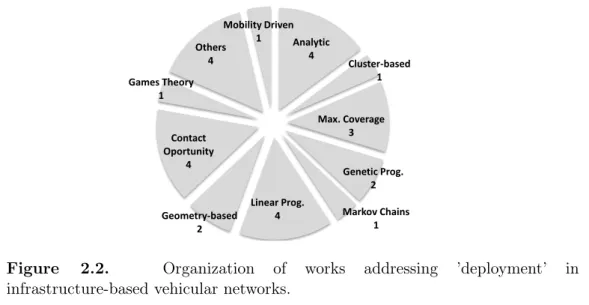
2.1 Number of articles addressing ’deployment’ of infrastructure for vehicular networks: The x-axis indicates year, while y-axis indicates number of published articles. . . 13 2.2 Organization of works addressing ’deployment’ in infrastructure-based

vehicular networks. . . 13 2.3 Articles presenting ’architectures’ for infrastructure-based vehicular

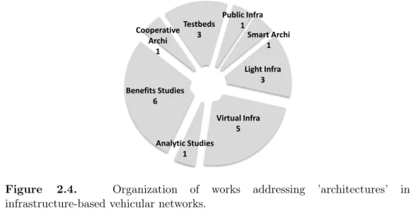
networks: x-axis indicates year, while y-axis indicates number of published works. . . 22 2.4 Organization of works addressing ’architectures’ in infrastructure-based

vehicular networks. . . 23 2.5 Number of published articles addressing ’communication’ in

infrastructure-based vehicular networks: x-axis indicates year, while y-axis indicates number of published works. . . 31 2.6 Organization of works addressing ’communication’ in infrastructure-based

vehicular networks. . . 32

3.1 Probabilistic model. A generic vehicle in intersection A has 40% of probability to reach B, 30% to reach C and 30% to reach D when t = 1. If the vehicle chooses C, when t = 2 the vehicle has 85% of probability to reach E, 5% to reach F and 10% to reach G . . . 48 3.2 Projection of ﬂow. . . 48 3.3 Theoretical road network containing one way roads: vehicles move top-down

and left-right. . . 52 3.4 Theoretical road network: Each road has a diﬀerent level of traﬃc modeled

as a Poisson Process. . . 53 3.5 Theoretical road network: Matrix P holding turning ratios. . . 53

(14)

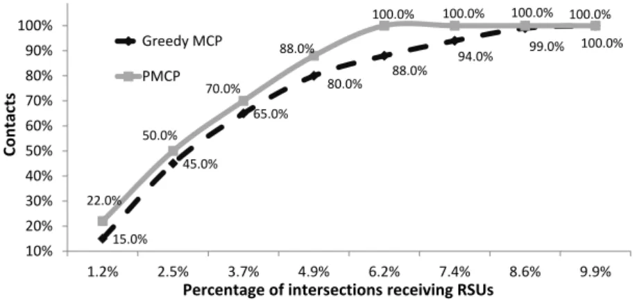
3.8 Theoretical road network: Extended matrixM. . . 55 3.9 9x9 Theoretical Grid-like Road Network. . . 59 3.10 Number of vehicle-to-infrastructure contacts: x-axis indicates number

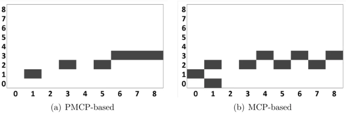
of intersections receiving roadside units (indicated as a percentage of intersections). The y-axis indicates number of contacts (indicated as a percentage of total trips). The graph is truncated in 100%. . . 60 3.11 Standard deviation. . . 61 3.12 Random Scenario: We use a 9×9-grid and random stochastic matrix. . . . 61 3.13 Location of RSUs according to both algorithms. . . 62 3.14 Coverage map based on distance: map characterizes all intersections in

terms of distance to nearest roadside unit in a 5-level scale: from black (distance= 0) to white (distance >4). . . 62 3.15 Histogram Vehicle-to-RSUs Distance: characterizes the position of each

vehicle according to the nearest RSU. . . 63 3.16 Cumulative percentage of vehicles x Distance to nearest roadside unit. . . . 63

4.1 Placing RSUs not in intersections. Maps from http://openstreetmap.org. 66

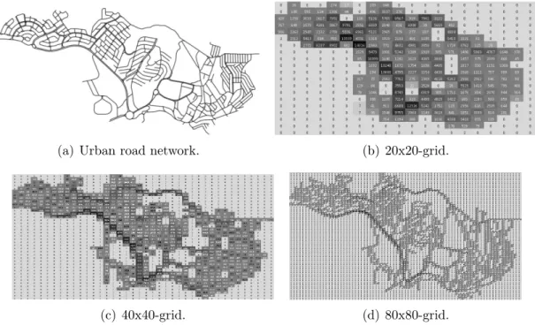
4.2 Plot shows the improvement in accuracy of the model when we increase the grid setup. . . 68 4.3 Urban cells composing a road network: projection of the ﬂow identiﬁes

vehicles moving in all four directions. . . 74 4.4 Distance traveled by each vehicle during 10 000s of simulation. . . 76 4.5 Map demonstrates the level of traﬃc in every road. Shadows indicate

popularity of the road. . . 77 4.6 Area x Trips: The x-axis indicates the covered area (i.e., the percentage of

urban cells fully covered by roadside units), while the y-axis indicates the number of trips. . . 78 4.7 Fairness in contacts opportunities: The plot shows the amount of distinct

vehicles crossing any of the ﬁve most important partitions during the simulation. The x-axis indicates the grid setup. The y-axis indicates the number of distinct vehicles as a percentage of total vehicles. The partitions are selected using MCP-based and PMCP-based. ’No Grid’ identiﬁes the result for a non-partitioned road network. . . 78 4.8 Number of V2I Contacts: The x-axis indicates incremental time intervals.

The y-axis indicates distinct contacts. . . 79

(15)

4.10 Vehicle-to-infrastructure contact time: x-axis indicates the grid setup, while

the y-axis indicates the total residence time. . . 80

4.11 PMCP: Standard deviation for V2I contact time. . . 81

4.12 MCP: Standard deviation for V2I contact time. . . 81

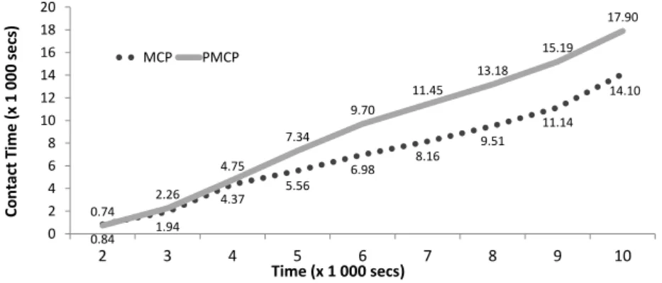
4.13 Average residence time (contact time): the x-axis indicates the time interval, while the y-axis indicates the V2I contact time. . . 82

4.14 V2I Contact Time Considering Dynamic Allocation. . . 82

4.15 V2I Contact Time: The x-axis shows the time interval. The y-axis shows the V2I contact time. . . 83

4.16 Evaluation segmented in time: x-axis indicates the time window. The y-axis indicates the V2I contact time. . . 84

4.17 Total V2I Contact Time for Distinct Grid Setups: The x-axis indicates the grid setup (from 20x20 to 800x800) for both MCP and PMCP. The y-axis indicates the sum of V2I contact time for all vehicles (x 1 000s). . . 85

4.18 Very small cells covering small pieces of a lane. . . 86

4.19 V2I Contact Time: 20x20-grid. The x-axis indicates the time window, while the y-axis indicates the total contact time. . . 87

4.20 Contact Time for Several Grid Setups. . . 88

4.21 Vehicles Contact Time. . . 89

4.22 Number of RSUs per vehicle for several grid setups. . . 90

4.23 Standard Deviation: Roadside Units per Vehicle: The x-axis indicates the grid setup, while the y-axis indicates the standard deviation. . . 90

4.24 Crossed Roadside Units Normalized to Standard Gaussian: Grid Setups 20x20, 40x40, and 60x60. . . 91

4.27 Percentage of Crossed Roadside Units for each Vehicle in Grid Setups 20x20, 100x100, 400x400: the x-axis indicates vehicle’s ID, while the y-axis indicates the percentage of Roadside Units. . . 93

5.1 Cologne’s Road Network. . . 96

5.2 Selection of locations to receive the roadside units: (a) Scenario; (b) MCP-kp selection; (c) PMCP-b selection. . . 100

(16)

5.5 Analysis of the Deployment Scenario. . . 103 5.6 Coverage Evaluation. The x-axis indicates the number of distinct vehicles

experiencing at least one V2I contact opportunity. The y-axis indicates the number of deployed roadside units. . . 104 5.7 Redundant Coverage. The x-axis indicates the roadside units ID (order

of deployment), while the y-axis indicates the number of vehicles crossing more than one RSU. . . 104 5.8 Percentage of Covered Vehicles x Covered Area. The x-axis shows the

number of deployed roadside units. The y-axis indicates the percentage of vehicles experiencing at least one V2I contact opportunity. . . 107 5.9 Improvements of MCP-g over PMCP-b, and PMCP-b over MCP-kp in terms

of the trips experiencing at least one V2I contact opportunity. The x-axis indicates the number of roadside units deployed. The y-axis indicates the percentage improvement. . . 108 5.10 Low Scale Deployment. The x-axis indicates the number of deployed

roadside units. The y-axis indicates the percentage of vehicles experiencing at least one V2I contact opportunity. . . 108 5.11 Percentage of vehicles reaching the infrastructure over time. The x-axis

indicates the time (×1 000s). The y-axis indicates the number of vehicles. 109 5.12 MCP-kp: Number of V2I contacts per RSU. The x-axis presents the RSUs in

the order of deployment. The y-axis indicates the total number of contacts for each roadside unit. . . 110 5.13 MCP-g: Number of V2I contacts per RSU. The x-axis presents the RSUs in

the order of deployment; The y-axis indicates the total number of contacts for each roadside unit. . . 110 5.14 PMCP-b: Number of V2I contacts per RSU. The x-axis presents the RSUs

in the order of deployment; The y-axis indicates the total number of contacts for each roadside unit. . . 111 5.15 Number of crossed RSUs per vehicle. The x-axis indicates the amount of

RSUs crossed. The y-axis indicates the number of vehicles (logarithmic scale).111 5.16 Road network and layout of roadside units for MCP-kp, PMCP-b, and MCP-g.112 5.17 Histogram presenting distribution of probabilities in P: x-axis indicates

turning probability, while y-axis indicates number of intersections. Four bars indicate the probability of a vehicle moves: up, down, left, or right. . 114

(17)

5.19 V2I Contact Opportunities: Figure highlights presents the V2I contact opportunities for several grid setups. 0.5% of the urban cells receive roadside units. . . 115 5.20 V2I Contact Time for Distinct Grid Setups: The x-axis indicates the grid

setup, while the y-axis indicates the contact time in millions of seconds (x1 000 000s). . . 116 5.21 Average V2I Contact Opportunities: The x-axis indicates the grid setup,

while the y-axis indicates the average number of V2I contacts. . . 116 5.22 Contacts in Intervals of 1,000s. The x-axis indicates time intervals, while

y-axis indicates the number of distinct vehicles reaching the infrastructure. 119 5.23 Distinct Vehicles: Distance from Optdv. The x-axis indicates time interval,

while y-axis indicates the distance from PMCP-based and MCP-based to Optdv in terms of distinct vehicles reaching the infrastructure. . . 120

5.24 Distinct Vehicles per Roadside Unit (500 RSUs). The x-axis indicates the RSU’s ID, while y-axis indicates the number of distinct vehicles crossing the roadside unit. . . 121 5.25 Vehicles Contact Time for 250 RSUs: x-axis indicates the RSU’s ID, while

y-axis indicates global vehicle-to-infrastructure contact time. . . 121 5.26 Contacts per Roadside Unit (250 RSUs): x-axis indicates the roadside unit’s

ID, while y-axis indicates the number of vehicle-to-infrastructure contacts. 122 5.27 Contacts per Roadside Unit (250 RSUs): x-axis indicates the roadside unit’s

ID, while y-axis indicates the number of vehicle-to-infrastructure contacts. 122 5.28 Roadside units crossed per vehicle: x-axis indicates the number of roadside

units crossed per vehicle, while y-axis indicates the percentage of vehicles. 123 5.29 Roadside units crossed per vehicle: x-axis indicates the number of roadside

units crossed per vehicle, while y-axis indicates the percentage of vehicles. 123 5.30 Distinct Vehicles Contacting Infrastructure: x-axis indicates grid setup,

while y-axis indicates the percentage of distinct vehicles contacting the infrastructure at least once. . . 125 5.31 Processing time for PMCP-based and MCP: x-axis indicates grid setup,

while y-axis indicates time in seconds. . . 126 5.32 Processing time for PMCP-based and MCP: x-axis indicates grid setup,

while y-axis indicates time in seconds. . . 126 5.33 Simulation Work Flow. . . 129

(18)

of vehicles experiencing at least one V2I contact opportunity. . . 130

5.35 Improvements of MCP-g over FPF, and FPF over MCP-kp in terms of the trips experiencing at least one V2I contact opportunity. The x-axis indicates the number of deployed roadside units. The y-axis indicates the percentage improvement. . . 132

5.36 Low Scale Deployment. The x-axis indicates the number of deployed roadside units. The y-axis indicates the percentage of vehicles experiencing at least one V2I contact opportunity. . . 132

5.37 MCP-kp: Number of V2I contacts per RSU. The x-axis presents the RSUs in the order of deployment. The y-axis indicates the total number of V2I contacts for each RSU. Plot shows the total V2I contacts (continuous line) and the number of V2I distinct vehicles contacts. . . 133

5.38 MCP-g: Number of V2I contacts per RSU. The x-axis presents the RSUs in the order of deployment. The y-axis indicates the total number of V2I contacts for each RSU. Plot shows the total V2I contacts (continuous line) and the number of V2I distinct vehicles contacts. . . 134

5.39 FPF: Number of V2I contacts per RSU. The x-axis presents the RSUs in the order of deployment. The y-axis indicates the total number of V2I contacts for each RSU. Plot shows the total V2I contacts (continuous line) and the number of V2I distinct vehicles contacts. . . 134

5.40 Number of crossed RSUs per vehicle. The x-axis indicates the amount of RSUs crossed. The y-axis indicates the number of vehicles (log₁₀). . . 135 5.41 Road network and layout of roadside units for: MCP-kp, MCP-g, and FPF. 136

6.1 Layout of Roadside Units: Figure shows the layout of roadside units for deployments considering time windows of 1 000s. . . 140 6.2 Vehicles Presenting V2I Contact Over Time. . . 142

6.3 Vehicles Arrival: Figure presents the number of new vehicles joining the Cologne scenario each 1 000s. . . 143

6.4 Global V2I Contact Opportunities: Figure presents the number of ’active vehicles’ × ’covered vehicles’ in the Cologne scenario. The x-axis indicates time, while the y-axis indicates the percentage of vehicles presenting at least one V2I contact opportunity. . . 144

(19)

presenting at least one V2I contact opportunity. . . 144

6.6 Deployment Performance During the Network Operation. The x-axis indicates time, while the y-axis indicates the number of distinct vehicles presenting contact opportunities as a percentage of the total number of activated vehicles. . . 145

6.7 Improvements of Hybrid Windowed Deployment over Static Deployment. . 146

6.8 Percentage of Stationary RSUs in hybrid deployment: Figure presents the number of roadside units not changing their locations in consecutive time windows. The x-axis indicates consecutive time windows, while the y-axis indicates the percentage of stationary roadside units. . . 147

6.9 V2I Contact Time: Figure indicates V2I contact time for HWD, SD and HCD. The x-axis indicates the time window, while the y-axis indicates the contact time (x1 000s). . . 148

6.10 V2I Contact Time: Figure indicates contact time as a percentage of the maximum contact time achieved for a given time window. . . 149

6.11 Average Displacement per RSU in meters. . . 150

6.12 Duration of Contact Opportunities. . . 151

A.2 Example of LaNPro operation. . . 180

A.1 Traﬃc light: scheduler selects between standard module and LaNPro according to the level of traﬃc. . . 180

A.3 LaNPro Organization. . . 182

A.4 Intersections considered during experiments: 2-4 lanes. . . 185

A.5 Probability of collisions for intersections composed from 2 to 4 lanes as we change safety margin (0m; 10m; 20m). . . 186

A.6 (a) Evaluation of the amount of vehicles stopping on a red light when the intersection has a static traffic light: low traffic incurs in increased traffic light stops. (b) Interruption of LaNPro: LaNPro routes all trafficλ ≤0.10. (c) Fluctuation of the queue of vehicles: LaNPro presents tiny queues for λ= 0.10, being able to route all traffic. . . 188

C.1 Published Articles per Year (Jan. 2003 to Feb. 2014). The x-axis indicates year, while y-axis indicates number of published works composing our sample.194

(20)

sample. . . 194

C.3 Evolution of Articles per Publisher (Jan. 2003 to Feb. 2014). The x-axis indicates year, while y-axis indicates number of published articles. Figure shows the evolution for ACM, IEEE, and Elsevier. . . 195

C.4 Number of articles per class: 27 works proposing deployment strategies; 22 works investigating architectures; and, 19 works proposing solutions for improving communication. . . 195

C.5 Evolution of published articles per year (2003-2014): x-axis indicates year, while y-axis indicates number of works (architecture, deployment, and communication). . . 196

C.6 Wordle of 2003-2004 abstracts. . . 197

C.11 Wordle of 2013 - Feb.2014 abstracts. . . 201

C.12 Citations per year: x-axis indicates year, while y-axis indicates the sum of citations from all articles published that year. Snapshot of Feb. 2014. . . . 202

C.13 Average citations per year: x-axis indicates year, while y-axis indicates average citations for all articles published that year. Snapshot of Feb. 2014. 202 C.14 Histogram presenting Citations per Articles: x-axis indicates number of citations, while y-axis indicates percentage of articles: 19.1% of articles received just 1 citation. . . 203

C.15 Players. . . 203

C.16 Conferences and Journals. . . 204

(21)

1 List of Symbols. . . xxiv

2.1 Articles of Deployment of Infrastructure for Vehicular Networks . . . 38

2.2 Articles of Communication for Infrastructure-Based Vehicular Networks . . 39

2.3 Articles of Architectures for Infrastructured Vehicular Communication. . . 40

4.1 Computational Complexity. . . 73

4.2 Grid Setups. . . 85

4.3 Contact Time Characterization: Intervals of 1 000s. . . 89

4.4 Number of crossed roadside units per vehicle. . . 91

5.1 Covered Area x Covered Vehicles. . . 107

5.2 Statistical Description of P . . . 113

5.3 Covariance of P . . . 113

5.4 Deployment Features . . . 114

5.5 Distinct Vehicles: PMCP-based and Optimum Deployment . . . 119

5.6 Percentage of distinct vehicles reaching infrastructure. (*) Vehicles presenting very high number of contacts. . . 124

5.7 Percentage of distinct vehicles reaching infrastructure. . . 124

5.8 Covered Area x Covered Vehicles. . . 131

5.9 Distinct-and-Covered Vehicles per Roadside Unit. . . 135

6.1 Percentage of Stationary Roadside Units. . . 147

6.2 Absolute V2I Contact Time. . . 148

6.3 Relative V2I Contact Time. . . 149

6.4 Characterizing the Mobility of RSUs. . . 150

6.5 Duration of Contact Opportunities. . . 151

C.1 Comparing citations per classes. . . 202

(22)

(23)

1 MCP-g: Greedy Solution (requires knowledge of trajectories). . . 44 2 MCP-based (without knowledge of trajectories). . . 45 3 PMCP-based . . . 47 4 Partition the Road Network. . . 70 5 Translate Real Coordinates To Grid Coordinates. . . 70 6 Compute Density of Vehicles in Grid. . . 71 7 Compute Migration Ratios in Grid. . . 72 8 Adapting Deployment Algorithms to Partitions. . . 99 9 FPF: Full Projection of the Flow Deployment. . . 128 10 Scheduler Algorithm. . . 181 11 LaNPro Algorithm. . . 184

(24)

Mi,j Bi-dimensional matrix holding number of vehicles at intersection of roads i

and j;

Pi,j Stochastic matrix holding turning ratio. Pi,j indicates the probability that

vehicles traveling on roadi turn into road j;

Pu

i,j Bi-dimensional matrix holding the likelyhood of vehicles moving up at

intersection (i, j);

Pd

i,j Bi-dimensional matrix deﬁned over1..n,1..n holding the likelyhood of vehicles

moving down at intersection (i, j);

Pr

moving right at intersection (i, j);

Pl

moving leftat intersection (i, j);

C_M,P,k_Γ Represents the projection of the ﬂow for all roads belonging to the road network considering the deployment of the kth _{roadside unit belonging to the solution}

setΓ. P FP

m,γ ∀m∈M, whereγ is the kth element of Γ;

Λ Bi-dimensional matrix holding the projected ﬂow of vehicles;

α Number of roadside units to be deployed;

Γ Solution set, i.e., intersections of urban cells receiving roadside units;

S Bi-dimensional matrix holding the sorted values ofM. |S|=|M|;

̺ Geographical map of the road network;

ψx Number of horizontal urban cells of the road network; ψy Number of vertical urban cells;

∆ Grid representing road network;

T Mobility trace;

τ Element of T;

G Mobility trace converted to grid coordinates;

K Set of vehicles (Chapter 6);

C Road network partitions (Chapter 6);

M Trajetories (Chapter 6);

A Urban cells receiving roadside units (Chapter 6);

V ’Covered’ vehicles;

λ Threshold of low traﬃc; (Chapter 7)

µ Interval (in minutes) for detecting low traﬃc (Chapter 7);

η Maximum size of the vehicle queue (Chapter 7);

ϑ Traﬃc light Id (Chapter 7);

(25)

Resumo ix

Abstract xi

List of Figures xiii

List of Tables xxi

1 Introduction 1

1.1 Infrastructure for Vehicular Networks . . . 2 1.2 Infrastructure Deployment . . . 4 1.3 Objectives and Intended Contributions . . . 6 1.4 Overview of Our Solution . . . 7 1.5 Overview of the Next Chapter . . . 10

2 Background 11

2.1 Methodology . . . 11 2.2 Deployment . . . 12 2.2.1 Analytic Studies . . . 15 2.2.2 Clustering Strategies . . . 16 2.2.3 Contact Opportunity . . . 16 2.2.4 Markov Chains . . . 18 2.2.5 Game Theory . . . 18 2.2.6 Genetic Algorithm . . . 18 2.2.7 Geometry-based Heuristics . . . 18 2.2.8 Linear Programming . . . 19 2.2.9 Strategies Based on Maximum Coverage . . . 20 2.2.10 Mobility-Driven Deployment . . . 20 2.2.11 Others . . . 21

(26)

2.3.1 Analytic Studies . . . 24 2.3.2 Benefits of Incorporating an Infrastructure . . . 24 2.3.3 Cooperative Architectures . . . 26 2.3.4 Light Architectures . . . 26 2.3.5 Publicly Available Infrastructure . . . 27 2.3.6 Smart Architectures . . . 27 2.3.7 Testbeds . . . 27 2.3.8 Virtual Infrastructure . . . 29 2.3.9 Remarks . . . 31 2.4 Communication . . . 31 2.4.1 Analytic Studies . . . 31 2.4.2 Infrastructure Benefits in Communications . . . 33 2.4.3 Infrastructure-based Data Dissemination . . . 33 2.4.4 Quality of Service . . . 33 2.4.5 Network Handoff . . . 34 2.4.6 Protocols for Infrastructure-based Vehicular Networks . . . 34 2.4.7 Routing in Infrastructure-based Vehicular Networks . . . 34 2.4.8 Security . . . 35 2.5 Physical Communication: 4G or DSRC . . . 36 2.6 Remarks . . . 37 2.7 Overview of the Next Chapter . . . 37 2.8 List of Selected Articles . . . 37

3 Grid-Based Road Network 41

3.1 Maximum Coverage Problem . . . 43 3.2 Probabilistic Maximum Coverage Problem . . . 45 3.2.1 Projection of the Flow . . . 47 3.3 Analytic Model for the Theoretical Grid Road Network . . . 51 3.3.1 Model #1: One Way Roads and Absence of Sinks . . . 51 3.3.2 Model #2: One Way Roads with Sinks . . . 56 3.4 Analytic Formulation of Infrastructure Deployment . . . 57 3.5 Simulations and Results . . . 58 3.5.1 Trips . . . 60 3.5.2 Allocation of Roadside Units . . . 60 3.5.3 Coverage Map . . . 61

(27)

3.7 Overview of the Next Chapter . . . 64

4 Real Road Network and Random Flow Deployment 65

4.1 Partitioning Road Networks . . . 67 4.2 Algorithmic Description . . . 69 4.3 Adapting the Flow Projection to Urban Cells . . . 73 4.4 Methodology . . . 75 4.4.1 Vehicles Flow Characterization . . . 76 4.5 Experiments S1: PMCP-based and MCP-based over Partitions . . . 77

4.5.1 Deployment Eﬃciency . . . 77 4.5.2 Fairness in Contacts Opportunities . . . 78 4.5.3 Cumulative Distinct Contacts Over Time . . . 79 4.5.4 Vehicle-to-Infrastructure Contact Time . . . 80 4.5.5 Cumulative Contact Time . . . 81 4.5.6 Dynamic Deployment of Roadside Units . . . 81 4.5.7 Dynamic MCP-based x Static MCP-based . . . 83 4.5.8 Remarks . . . 83 4.6 Experiments S2: Comparing Grid Setups . . . 84

4.6.1 Over-Partitioning . . . 85 4.6.2 Characterizing the Contact Time . . . 86 4.6.3 Crossed Roadside Units . . . 87 4.6.4 Comparison of Crossed Roadside Units . . . 89 4.7 Analysis . . . 93 4.8 Overview of the Next Chapter . . . 94

5 Realistic Flow Deployment 95

5.1 Review of Deployment Algorithms . . . 97 5.2 Comparison between PMCP-b and MCP-kp . . . 100 5.2.1 Evaluation Over a Synthetic Road Network . . . 100 5.2.2 Selection of Locations made by PMCP-b and MCP-kp . . . 102 5.2.3 Coverage Evaluation . . . 103 5.2.4 Redundant Coverage . . . 104 5.2.5 Discussion . . . 105 5.3 Comparison of PMCP-based, MCP-based and MCP-g . . . 105 5.3.1 Covered Vehicles x Covered Area . . . 106

(28)

5.3.4 Number of V2I Contacts per Roadside Unit . . . 109 5.3.5 V2I Contacts per Vehicle . . . 111 5.3.6 Roadside Units Layout . . . 112 5.3.7 Characterizing Migration Ratios . . . 112 5.4 Road Networks Partition: Evaluation On a Realistic Scenario . . . 113 5.4.1 V2I Contact Opportunities . . . 114 5.4.2 V2I Contact Time . . . 115 5.4.3 Average V2I Contact Opportunities per Vehicle . . . 116 5.4.4 Analysis . . . 116 5.5 Optimal Deployment . . . 117 5.5.1 Distinct Vehicles per Time Interval . . . 119 5.5.2 Distinct Vehicles Crossing Each Roadside Unit . . . 120 5.5.3 Contact Time . . . 120 5.5.4 Roadside Units Crossed per Vehicles . . . 123 5.5.5 Distinct Grid Setups . . . 124 5.5.6 Processing Time . . . 125 5.6 Full Projection of the Flow . . . 125 5.6.1 FPF: Full Projection of the Flow Deployment . . . 127 5.6.2 Evaluation On a Realistic Scenario . . . 128 5.6.3 Roadside Units Layout . . . 136 5.7 Remarks . . . 136 5.8 Overview of the Next Chapter . . . 138

6 Hybrid Deployment 139

6.1 Deployment Algorithm . . . 141 6.2 V2I Contacts for Distinct Grid Setups . . . 142 6.3 Characterizing the Cologne Scenario . . . 142 6.4 Global V2I Contact Opportunities . . . 143 6.5 Memoryless V2I Contacts Over Time . . . 144 6.6 Cumulative V2I Contacts Over Time . . . 145 6.7 Improvements of Hybrid Windowed Deployment over Static Deployment 146 6.8 Share of Stationary Roadside Units . . . 147 6.9 Absolute V2I Contact Time . . . 148 6.10 Relative V2I Contact Time . . . 148 6.11 Displacement of Mobile Roadside Units . . . 149

(29)

7 Final Remarks 153

7.1 Future Works . . . 156

Bibliography 159

Appendix A Non-Stop Driving-Thru Low Traffic Intersections 177

A.1 Related Work . . . 178 A.2 Overview of LaNPro . . . 179 A.3 Main Functionalities of LaNPro . . . 182 A.4 Evaluation of the Collision Risk . . . 182 A.5 Managing Intersections . . . 183 A.6 LaNPro Algorithm . . . 183 A.7 Results . . . 185 A.8 Remarks . . . 190

Appendix B Publications & Awards 191

B.1 Award . . . 191 B.2 Patent Application . . . 191 B.3 Journals . . . 191 B.4 International Conferences . . . 192 B.5 Brazilian Conferences . . . 192

Appendix C Complementary Study of the Literature 193

C.1 Classiﬁcation . . . 193 C.2 Overview of Research . . . 196 C.3 Citations . . . 201 C.4 Characterizing Players: Universities & Labs . . . 203 C.5 Conferences & Journals . . . 204

(30)

(31)

Introduction

Nowadays, traffic is one of the most important urban issues, and it is becoming unmanageable in large metropolitan areas. As an example, the amount of vehicles increases annually by rates of at least 10% in most developing countries, thus doubling the number of cars every seven years (Gakenheimer, 1999). Furthermore, traffic raises other areas of concern, such as environmental pollution, public health and safety. An Intelligent Transportation System would help to alleviate the problems of the transportation sector. By embedding computing devices into cars, roads, streets, and transit equipment such as street signs, radars, traffic cameras and others, we will be capable of ’digitalizing’ the transportation system (Macedo et al., 2012; Oliveira et al., 2013). Applications are endless: driver assistance for faster, less congested and safer roads; more efficient use of the transportation system; more efficient planning of routes and control of the traffic flow; secure and greener traffic through digital driver assistance; and better planning and evolution of the system as a whole due to the availability of historical data, based on traffic and utilization trends detected via data mining techniques. As indicated by the European Transportation Policy (2001), the use of Intelligent Transportation Systems is one of the key technologies for improving the safety, efficiency and environmental friendliness of the transport industry.

An Intelligent Transportation System is grounded on a sophisticated communication network receiving data from several entities composing the traﬃc system. Data is processed and translated into useful information and recommendations to assist users of the transportation system and transit authorities. Such sophisticated communication network is commonly referred as a vehicular network (Hartenstein and Laberteaux, 2008; Youseﬁ et al., 2006; Jakubiak and Koucheryavy, 2008).

A vehicular network is a network connecting vehicles in order to provide a

platform for future deployment of large-scale and highly mobile applications. Mobility

(32)

is probably the most intrinsic and distinguished feature of vehicular networks. In such dynamic network, localizing vehicles is a necessary challenge (Boukerche et al., 2008) in order to maximize the network beneﬁts. Future position of vehicles is almost non-deterministic and previous warning of trajectories by vehicles is an unrealistic assumption. Given the automobile’s role as a critical component in peoples’ lives, embedding software-based intelligence into them has the potential to drastically improve drivers’ quality of life (Gerla et al., 2006). Leveraging wireless communication in vehicles has fascinated researchers since the 1980s (Kawashima, 1990). A few years later, as a consequence of the cellular revolution, voice services have become commonplace and ubiquitous, and the attention of researchers has shifted to wireless communication (Frenkiel et al., 2000).

In a vehicular network, communication may happen in a direct and completely distributed basis where vehicles exchange messages without any support infrastructure (vehicle-to-vehicle communication). Such kind of ad hoc communication has been extensively studied by the research community (Hartenstein and Laberteaux, 2008; Jakubiak and Koucheryavy, 2008). However, the ad hoc communication may become ineﬃcient due to the high mobility of vehicles, leading to very short contact times possibly reducing the network throughput. Additionally, communication also suﬀers in sparse areas such as highways, rural zones and low peak hours in city due to the lack of communicating pairs. High mobility also makes routing far complicated as we lack reliable means to infer future position of vehicles. Although communication may take place in a vehicle-to-vehicle basis, research demonstrates that a minimum support infrastructure may largely improve the overall efficiency of the

vehicular network (Kozat and Tassiulas, 2003; Gerla et al., 2006; Banerjee et al.,

2008; Reis et al., 2011; Mershad et al., 2012; Wu et al., 2012b).

1.1 Infrastructure for Vehicular Networks

In the context of vehicular networks, infrastructure is a set of specialized

communication devices supporting the network operation. Common properties

(33)

2013); data dissemination strategies (Lochert et al., 2007); data aggregation (Bruno and Nurchis, 2013); data scheduling (Shumao et al., 2009); gaming and streaming (Palazzi et al., 2008, 2009); gateway functionalities (Wu et al., 2005a; Gerla et al., 2006; Liang and Zhuang, 2012); hand-oﬀ optimizations (Ramani and Savage, 2005; Brik et al., 2005; Amir et al., 2006); localization of vehicles (Boukerche et al., 2008; Rosi et al., 2008); quality of service assurance (Luan et al., 2012); real time support (Korkmaz et al., 2010; Liu and Lee, 2010; Abdrabou et al., 2010); routing (Borsetti and Gozalvez, 2010; Annese et al., 2011; Mershad et al., 2012); security, privacy and reputation (Marmol and Perez, 2012; Fernandez Ruiz et al., 2010; Plobl and Federrath, 2008; Souza et al., 2009); and, support to multi-hop communication (Zhang et al., 2012).

Several technologies and devices may serve as roadside units. Banerjee et al. (2008) present an in-depth discussion and comparison of such technologies. Although most of the works consider stationary infrastructure, several researches (Jerbi et al., 2008; Luo et al., 2010; Annese et al., 2011; Mishra et al., 2011; Tonguz and Viriyasitavat, 2013; Sommer et al., 2013) propose mobile architectures (public transportation buses, cabs, ordinary vehicles). There are also proposals considering the use of low cost devices as an infrastructure (Luan et al., 2013), while another proposals consider the use external devices serving the vehicular network such as public available Wi-Fi connections (Marﬁa et al., 2007).

Throughout this thesis we conducted a Systematic Literature Review (SLR) on infrastructure-based vehicular networks from Jan. 2003 up to Feb. 2014 where we mapped the research evolution over the years, and the state-of-the-art in:

(a) Infrastructure deployment in vehicular networks;

(b) Vehicle-to-infrastructure communication;

(c) Architectures of infrastructure-based vehicular networks.

Our Systematic Literature Review captured 30 works addressing aspects of infrastructure deployment. When we analyze all these eﬀorts we conclude that they usually consider unrealistic road networks or unrealistic mobility, and such lack of realism implies in severe impreciseness in results reported by these works1 _{(Fiore and} Härri, 2008).

1

(34)

1.2 Infrastructure Deployment

Deployment of infrastructure is one of the most critical decisions when designing a vehicular network. Infrastructure deployment is the task of deﬁning the exact position of each roadside unit within the road network. A misleading deployment means waste of valuable resources and degradation of the network performance.

Infrastructure deployment for vehicular networks is an open problem. Given that high mobility is, perhaps, the most distinguished feature of vehicular networks, it must be the start point of a deployment strategy. Typically, deployment algorithms propose alternative ways to identify the most populated locations within the road network. Those selected locations receive roadside units. Although placing roadside units in densest places may seem reasonable at a first glance, the assumption fails when we consider that those vehicles composing the dense regions are originated from nearby, and the dense region is created as a result of merging flows. Figure 1.1 presents the realistic flow of vehicles in the city of Cologne (Germany), and we notice: (a) flows creating dense areas; and, (b) connectivity between dense areas. Intensity of black color indicates traffic level. From Figure 1.1(a) to Figure 1.1(f), we present the remaining road network after eliminating roads below an increasing minimum traffic threshold.

Selecting the densest places is a correct decision when nodes composing the network are stationary (or moving at very low speeds). But when dealing with high speed mobile nodes (i.e., vehicles) we must consider the mobility and the flow characteristics. Typically, dense regions do not appear as isolated islands, but they result from merging flows converging to attraction areas. Such issue indicates that dense regions tend to appear somehow interconnected, and vehicles traveling nearby dense areas have high probability of joining the main flow. Thus, when we consider just the concentration of vehicles to position the roadside units, we may incur in redundant coverage by deploying roadside units covering the same flow twice or more. Thus, we investigate the benefits of incorporating mobility information into deployment algorithms.

(35)

(a) Cologne road network: Original Flow. (b) Roads with traffic level > 30% of Max. level.

(c) Roads with traffic level > 40% of Max. level. (d) Roads with traffic level > 60% of Max. level.

(e) Roads with traffic level > 80% of Max. level. (f) Roads with traffic level > 90% of Max. level.

Figure 1.1. Figure illustrates merging flows converging to attraction areas.

Formally, we can formulate the deployment of infrastructure aiming to maximize the number of distinct vehicles contacting the infrastructure as follows:

Let G = (V, E) be a graph where V represents the set of roads of a given road network and E represents roads intersections. Let A={a1, a2, ..., ah}

(36)

byα. Γ← ∅ is our solution set, i.e., the position of each deployed roadside unit. C ← ∅ represents the set of ’covered’ vehicles, i.e., vehicles that have already reached any roadside unit during the trip. ∀a ∈ A do C ← C∪a

if a has crossed at least one of locations composingΓ: vehicle is considered ’covered’ if it reaches any roadside unit. Roadside units are deployed at locations Γ.

Our goal is to ﬁnd Γ⊆Gwhere |Γ| ≤α and |C| is maximum.

Our Systematic Literature Review (Chapter 2) also reveals that previous deployment works do not agree on a strategy to represent the road network, and just two works (Cheng et al., 2013; Patil and Gokhale, 2013) consider basic concepts of Geographical Information Systems (GIS). Lacking a standard representation of road networks makes comparison of results far complicated. Thus, we propose a strategy to represent road networks of arbitrary complexity.

We also exploit the Probabilistic Maximum Coverage Problem (PMCP) for infrastructure deployment over vehicular networks. A deployment strategy that selects the densest locations to receive the roadside units is, in fact, proposing a solution for Maximum Coverage Problem. Maximum Coverage Problemconsiders a collection of sets deﬁned over a domain of elements. These elements are distributed over a given number of sets. Each element may appear in more than one set. Sets of elements are static, thus elements do not migrate between sets. Goal is to select those α sets presenting maximum cardinality. Given that elements do not migrate between sets, Maximum Coverage Problem is not suitable to handle mobility. On the other hand:

Probabilistic Maximum Coverage Problem considers a collection of sets

deﬁned over a set of elements. These elements have a probability of belonging to a given set. Sets of elements are not static because elements are not tied to sets. Goal is to select those α sets presenting maximum expected cardinality. We highlight the application of the Probabilistic Maximum Coverage Problem as a contribution of this work because, as far as we know, Probabilistic Maximum Coverage Problem is exploited in just one work in the literature: Fan and Li (2011) apply Probabilistic Maximum Coverage Problem in order to maximize information propagation in social networks. Ultimately, information propagation is the ’mobility of information’.

1.3 Objectives and Intended Contributions

(37)

mobility information means that we do not rely on individual vehicles trajectories. Only information we have are migration ratios between adjacent urban cells. Our solution models the allocation of roadside units as a Probabilistic Maximum Coverage Problem, a probabilistic instance of the traditional Maximum Coverage Problem, and we consider the position of each vehicle to be no longer deterministic, but a probabilistic position given by function f : {c1, c2, P} −→ R that returns the probability that a vehicle

located at urban cell c1 will migrate to urban cell c2 considering the mobility model

P. Urban cells are micro-areas composing the road network. Union of all urban cells is the road network itself. Chapter 4 presents an in-depth discussion of urban cells, road network partitioning, and experimental results considering the road networks partitioning.

Splitting the road network into a set of discrete urban cells simpliﬁes the detection of sources, destinations, and migration ratios. Basic mobility patterns are highlighted by splitting the road network into just a few urban cells. More sophisticated mobility patterns are highlighted by increasing the number of urban cells covering the road network. Splitting the road network into urban cells is the core of our proposed strategy to represent road networks of arbitrary topology.

Thus, our intended contribution with this thesis is:

Design of a deployment algorithm employing a new paradigm of mobility information.

Next section presents an overview of our solution.

1.4 Overview of Our Solution

In this work2 _{we design a novel infrastructure deployment algorithm for vehicular} networks. Our algorithm uses a mobility model based on global behavior, i.e., we exploit the vehicles’ migration ratios between urban cells composing the road network. Our work is motivated by the study of Trullols et al. (2010), which demonstrates that when we know the trajectories of vehicles in advance, we achieve close-to-optimum deployment performance. However, when we lack information of vehicles trajectories, performance of Maximum Coverage Problem is strongly aﬀected. Because full knowledge of vehicles trajectories implies in several privacy (and also practical) issues, we have turned our attention to improve the performance of Maximum

2

(38)

Coverage deployment by using a mobility model describing the global behavior, instead of individual behavior.

InChapter 2we present a Systematic Literature Review of works published from

Jan. 2003 to Feb. 2014 in IEEExplore, ACM Digital Library and Elsevier Science Direct in order to characterize the evolution of the research in infrastructure-based vehicular networks.

In Chapter 3 we develop our deployment algorithm in a theoretical grid-based

road network with randomized ﬂows (Chun et al., 2010; Larson, 1982; McNeil, 1968; Gerlough and Schuhl, 1955). We assume roadside units always positioned at roads intersections. We model the position of each vehicle as a functionf :{c1, c2, P} −→R

that returns the probability that a vehicle located at urban cell c1 migrates to urban

cell c2 considering the mobility model P. Our mobility model lies on the assumption

that vehicles do not have a deterministic position. Instead, vehicles have a probability of being at a given position in a given instant of time. By using the mobility model we deﬁne the deployment of infrastructure as a Probabilistic Maximum Coverage Problem. However, because we do not assume previous knowledge of vehicles trajectories, we are not able to truly solve neither PMCP, nor MCP. Instead of it, we propose constructive heuristics to approximate both problems solutions.

In Chapter 4 we generalize our deployment algorithm to handle real road

networks, and we also perform a worst-case analysis of the deployment performance considering a PMCP-based approach, and a MCP-based one. We use the road network of a Brazilian city3 _{using synthetically generated flows in order to perform a worst-case} analysis of deployment efficiency. We partition the road network into a set of adjacent same size urban cells. Once the road network is partitioned we discard the real road network and we manipulate the flow between adjacent urban cells. We also evaluate the benefits of using dynamic deployment of roadside units. Although dynamic deployment is not possible with stationary infrastructure, we have already mention the existence of several works (Jerbi et al., 2008; Luo et al., 2010; Annese et al., 2011; Mishra et al., 2011; Tonguz and Viriyasitavat, 2013; Sommer et al., 2013) proposing the adoption of a virtual-and-mobile infrastructure to support the vehicular communication. Thus, contributions of this chapter are: (a) characterizing the efficiency of partitioning the road network; (b) characterizing the worst-case deployment performance of a PMCP-based and MCP-based approaches.

In Chapter 5 we evaluate our deployment algorithm using a real road network

(750km2_{) and a realistic vehicular trace. The results demonstrate 89.6% of the vehicles}

3

(39)

experience at least one V2I contact by covering just 2.5% of the entire road network. Now we compare PMCP-based to MCP-based and also MCP-g (greedy solution for MCP).

After that, we reevaluate the partition technique considering MCP-g presented in Algorithm 1. MCP-g is the greedy solution for the Maximum Coverage Problem. Thus, it relies on previous knowledge of vehicles trajectories. Our selection of MCP-g is based on the fact that MCP-g achieves close-to-optimum coverage (Section 5.5). We propose the deployment of roadside units covering just 0.5% of the road network. Thus, after partitioning the road network we select the 0.5% of the most promising urban cells to receive the roadside units.

Then, we propose an Integer Linear Programming Formulation (Optdv) for the

deployment. We compare our PMCP-based approach, MCP-based, and Optdv through

several experiments. Our experiments reveal that our Integer Linear Programming Formulation is able to solve instances presenting large number of roadside units. Thus, we have assumed the deployment of α=500 roadside units (coverage of 5% of the entire road network). We were not able to solve instances presenting lower number of roadside units, namely α=250, and α=50 without oﬀering initial solutions to the model. We have evaluated our Integer Linear Programming Formulation oﬀering initial solutions computed using the well-know greedy solution for MCP (MCP-g) presented in Algorithm 1. CPLEX was not able to improve the MCP-g solution, but it outputs that optimal solution is at most 3.5% above the MCP-g solution.

In Chapter 6 we investigate an architecture composed of stationary and mobile

roadside units. It is a common sense that traffic fluctuates: thus, an architecture employing just stationary roadside units might not be able to properly support the network operation all the time. Similarly, an architecture composed just of mobile roadside units makes a few sense when we consider that the road network does not change that often. In other words, traffic fluctuations are limited by its subjacent road network. As major roads counts on higher transportation capacity, they tend to be very popular routes, and they are natural candidates for receiving stationary roadside units. And mobile roadside are highlighted as ideal solutions to handle in-borders traffic. In order to improve the deployment performance, we may rely on hybrid deployment strategies employing sets of stationary and mobile roadside units. Stationary roadside units act as a main backbone for data dissemination covering the most important regions of an urban area (i.e., regions known as always presenting relevant traffic). On the other hand, we may rely on mobile roadside units to address traffic fluctuations.

(40)

designed to operate under low traﬃc conditions usually found in small cities and during early hours of morning. In Appendix B we present our publications and awards. Finally, in Appendix C we expand our systematic literature review.

1.5 Overview of the Next Chapter

(41)

Background

In this chapter we review and characterize works published in IEEE, ACM and Science Direct (Elsevier) from Jan. 2003 to Feb. 2014 addressing infrastructure-based

vehicular networks. We have selected a set of 68 articles published in conferences

and journals, and our goal is to identify the solutions proposed in the literature through a Systematic Literature Review (SLR). This chapter is organized as follows: Section 2.1 presents our methodology. Sections 2.2 to 2.4 describes the selected works. Section 2.6 concludes the chapter.

2.1 Methodology

Studies of this research have been collected in electronic databases meeting the following criteria: (a) peer reviewed articles; (b) search engine by keywords per ﬁeld; (c) full access to articles; and (d) recognized reputation in publishing high quality content. Resulting list of selected databases is: ACM Digital Library (http://portal.acm. org/); IEEEXplore (http://www.ieeexplore.ieee.org/); Elsevier Science Direct

(http://www.sciencedirect.com/). We have deﬁned our period of interest as Jan.

2003 to Feb. 2014, and the search string as:

((infrastructure OR roadside OR rsu OR dissemination points OR access points) AND (vehicular networks OR vanet))

Using the search string we have retrieved all articles with matches in title, abstract or keywords using the search engine of each publisher (ACM, IEEE, Elsevier). In order to validate the search string we have conducted an investigative review in order to identify false-negatives (articles related to our target but not retrieved by the search

(42)

string). The investigative review is performed in three steps: (i) Search via Google Scholar1_{; (ii) Search via Mendeley}2 _{Tool; (iii) Manual inspection of the bibliography of} the selected articles from 2011 up to 2014.

By following the steps of a SLR (Kitchenham, 2004; Kitchenham and Charters, 2007), we have established a four-step process with diﬀerent review processes, namely: (a) remove duplicate papers; (b) remove papers not dealing with infrastructure aspects of vehicular networks; (c) eliminate papers by scanning through the full text in order to check whether the inclusion or exclusion criteria were met; (d) full text analysis in articles meeting inclusion criteria. Inclusion and exclusion criteria shown below were used to narrow the search to relevant papers.

• Inclusion criteria: papers describing researches on infrastructure-based

vehicular networks;

• Exclusion criteria: short papers, editorials, posters, introductions of keynotes,

mini-tracks, studies in languages other than English.

In the following sections we describe the selected articles: Section 2.2 presents

deployment works. Section 2.3 presents architecture works. Section 2.4 presents

communicationarticles.

2.2 Deployment

In this section we present works addressing the deployment of infrastructure for vehicular networks. Until 2006, the research community is focused on low level aspects of ad hoc communication. Initial deployment eﬀorts focus on bringing Internet into vehicles. Soon the research community realizes that a communication infrastructure is able to oﬀer much more than Internet access. In a attempt to reduce the high costs of the deployment, the research community evaluates: (i) use of public available Wi-Fi networks (spread over urban centers) to support the vehicular communication; (ii) design of virtual-and-mobile infrastructures composed of vehicles and buses; (iii) the use of cheap devices acting as roadside units.

In 2007-2008 we notice the initial eﬀorts presenting deployment algorithms. Such eﬀorts propose strategies maximizing the vehicle-to-infrastructure contact probabilities (Li et al., 2007), or content distribution (Rosi et al., 2008). There are also analytic

1

http://scholar.google.com

2

(43)

studies (Nekoui et al., 2008), and the application of genetic programming (Lochert et al., 2008). Figure 2.1 presents the number of published articles per year. The x-axis indicates year, while y-axis indicates number of published articles. Figure 2.2 presents the strategy used to solve the deployment.

0 0 0 0 0

1 3

1 5

2 6

7

2

0 2 4 6 8

2000 2003 2004 2005 2006 2007 2008 2009 2010 2011 2012 2013 2014

Deployment

Figure 2.1. Number of articles addressing ’deployment’ of infrastructure for vehicular networks: The x-axis indicates year, while y-axis indicates number of published articles.

Analytic 4

Cluster-based 1

Max. Coverage 3

Genetic Prog. 2 Markov Chains

1 Linear Prog.

4 Geometry-based

2 Contact Oportunity

4 Games Theory

1

Others 4

Mobility Driven 1

Figure 2.2. Organization of works addressing ’deployment’ in infrastructure-based vehicular networks.

• Linear Programming: eﬀorts proposing a linear programming (Gass, 1958;

(44)

linear inequality constraints. Its feasible region is a convex polyhedron, which is a set defined as the intersection of finitely many half spaces, each of which is defined by a linear inequality. Its objective function is a real-valued affine function defined on this polyhedron. A linear programming algorithm finds a point in the polyhedron where this function has the smallest (or largest) value if such a point exists;

• Maximum Coverage: eﬀorts modeling the allocation of infrastructure as a

Maximum Coverage Problem. Maximum Coverage is a classical problem in Computer Science. Basically, we have a collection of sets deﬁned over a domain of elements. These elements belong to some sets. One element may belong to more than one set. The goal is to select a collection of sets maximizing the cardinality of elements. A detailed discussion of the problem is found in (Cormen et al., 2001);

• Analytic Studies: eﬀorts proposing analytic formulations to model aspects

of the deployment, typically delay-bounded strategies for vehicle-to-vehicle and vehicle-to-infrastructure communications;

• Cluster-based: eﬀorts proposing deployment strategies based on data clustering

(Zaki and Meira Jr, 2014; Kaufman and Rousseeuw, 2009). Clustering is the task of grouping a set of objects in such a way that objects in the same group are more similar to each other than to those in other groups;

• Contact Opportunities: eﬀorts proposing deployment strategies in order to

maximize the vehicle-to-infrastructure contact probability;

• Markov Chains: eﬀorts proposing Markov Chains (Chung, 1967; Markov, 1971;

Meyn and Tweedie, 2009; Kemeny and Snell, 1960) to model the encounters of vehicles and the infrastructure. A Markov chain is a mathematical system that undergoes transitions from one state to another on a state space. It is a random process usually characterized as memoryless: the next state depends only on the current state and not on the sequence of events that preceded it;

• Game Theory: eﬀorts using concepts of Game Theory (Harsanyi and Selten,

(45)

logic, computer science, and biology. The subject ﬁrst addressed zero-sum games, such that one person’s gains exactly equal net losses of the other participant or participants. Today, however, game theory applies to a wide range of behavioral relations, and has developed into an umbrella term for the logical side of decision science;

• Mobility-Driven: eﬀorts proposing the use of vehicular mobility to assist the

deployment activity;

• Genetic Programming: eﬀorts using genetic programming (Koza, 1992;

Banzhaf et al., 1998) in order to find out better solutions (considering a given objective function). Genetic programming is an evolutionary algorithm-based methodology inspired by biological evolution to find computer programs that perform a user-defined task. Main operators used in evolutionary algorithms are crossover and mutation;

• Geometry-based: eﬀorts applying geometry concepts in order to deploy the

infrastructure.

• Others.

Sections 2.2.1 to 2.2.11 detail these works.

2.2.1 Analytic Studies

Nekoui et al. (Nekoui et al., 2008) propose an infrastructure for vehicular networks based on the conventional definition of the transport capacity. Authors develop a mathematical model where the destination nodes are chosen at random by the source nodes. Authors study the effect of infrastructure node deployment in the capacity of vehicular networks, and using analytical expressions they show that exploiting any number of infrastructure nodes beyond a certain amount enhances the achievable capacity. Although the authors propose to handle arbitrary topologies, they assume several simplifications in the mobility model.

Alpha Coverage (Zheng et al., 2009) provides worst-case guarantees on the interconnection gap while using signiﬁcantly fewer roadside units. A deployment of roadside units is considered α-covered if any simple path of length α on the road network meets at least one roadside unit. Authors compare theα-coverage with random deployment of roadside units.

(46)

into account important issues like vehicle deceleration, channel congestion, diﬀerent beacon frequencies, hidden node problem, and multi-lane traﬃc. The results indicate that on a 300km highway the rehealing delay is reduced by 70%, whereas the average number of rehealing hops is reduced by 68.4% when deploying 50 roadside units compared to an operation with no roadside unit. Authors conclude that: (i) the deployment of a small number of roadside units may achieve a substantial improvement when the vehicular network is sparse; (ii) the roadside units prevent the occurrence of the broadcast storm; and (iii) roadside units improve the message penetration time and packet delivery ratio, while reducing the delay.

Sou (Sou, 2010) also addresses the placement of roadside units at rural areas and roadways where the solutions must deal with the low density of vehicles and very large areas to be covered. The author proposes the deployment of the roadside units equally distanced from each other along a roadway enabling some roadside units to enter the power-saving mode in order to optimize the energy consumption. The work presents an algorithm to select the roadside units to enter the power-saving mode.

2.2.2 Clustering Strategies

Kchiche and Kamoun (Kchiche and Kamoun, 2010) apply clustering techniques to solve the roadside units’ allocation through a greedy algorithm based on the centrality of group in order to select the better locations for the infrastructure. The algorithm aims to maximize the performance of the message distribution system by reducing the global delay and the messages communication overhead. The authors also demonstrate that the centrality and the equidistance of the infrastructure are important features to improve the quality of the coverage. When considering just the ad-hoc communication, authors report an end-to-end delay of several minutes.

2.2.3 Contact Opportunity

(47)

Zheng et al. (Zheng et al., 2010) present the evaluation of a deployment strategy considering the contact opportunity. Contact opportunity measures the fraction of distance or time that a vehicle is in contact with the infrastructure. Authors argue that such metric is closely related to the quality of data service that a mobile user might experience while driving. Authors also propose a deployment algorithm intended to maximize the worst case contact opportunity under budget constraints. The solution is evaluated using computer simulations and a testbed in a university campus. Authors compare the results with two baseline algorithms: (i) Uniform

Random Samplingselects the location of the access points at random; (ii)Max-Min

Distance Sampling (Teng, 1995) starts at a randomly selected location, and at

each step allocates a new access point in order to maximize the minimum graph distance (in terms of shortest paths) from the elements already selected. Experimental results show that the deployment strategy achieves more than 200% higher minimum contact opportunity, 30%-100% higher average contact opportunity, and a signiﬁcantly improved distribution of average throughput when compared to Uniform Random Sampling and Max-Min Distance Sampling.

Lee and Kim (Lee and Kim, 2010) propose a greedy heuristic to place the infrastructure aiming to improve the vehicles connectivity while reducing the disconnections. The heuristic counts the amount of reached vehicles at each intersection by considering the transmission range of the roadside units. Each intersection is considered as a potential roadside unit location. Optimal locations are selected based on the number of vehicle reports (per minute locations reported by taxis to telematics system) received within the communication range of each roadside unit. Placement scheme considers only the taxi location reports, and it does not take into account speed, nor density of vehicles.

(48)

2.2.4 Markov Chains

Liu et al. (Liu et al., 2013) propose a new roadside units’ deployment strategy for ﬁle downloading in vehicular networks. The encounters between vehicles and roadside units are modeled as a time continuous homogeneous Markov chain. The road network is modeled as a weighted undirected graph, and the authors propose an algorithm for the deployment of roadside units.

2.2.5 Game Theory

Filippini et al. (Filippini et al., 2012) apply games theory to characterize the better strategy for competing providers to deploy the roadside units in order to maximize the revenue. The authors derive preliminary results evaluated via simulations. They consider a scenario with two operators deploying roadside units for distributing content along a road of lengthD. Each roadside unit is characterized by a coverage range R, which deﬁnes its service area, and by an application level goodputcfor content delivery. The goodput measure depends on the wireless technology, and on the communication protocols used for content delivery.

2.2.6 Genetic Algorithm

Lochert et al. (Lochert et al., 2008) study how the infrastructure may be used to improve the travel time of data over large distances. The authors present a multilayer aggregation scheme deﬁning landmarks. Cars passing landmarks record time travel, which is aggregated to infer the time travel between more distant landmarks. These aggregation steps are performed by the cars themselves in a completely decentralized basis whenever information that is a suitable basis for forming an aggregate becomes locally available. Minimal initial deployment of roadside units is handled by a genetic algorithm based on the travel time savings. Cavalcante et al. (Cavalcante et al., 2012) apply genetic programming to solve the deployment of dissemination points in vehicular networks. They start with an initial set of possible solutions that are combined across generations until some stop condition is reached. The authors model the problem as a Maximum Coverage and they impose a time limit.