Adverse selection with endogenous entry

FUNDAC

¸ ˜

AO GET ´

ULIO VARGAS

ESCOLA DE ECONOMIA DE S ˜

AO PAULO

AMANDA FORLIN

Adverse Selection with Endogenous

Entry

FUNDAC

¸ ˜

AO GET ´

ULIO VARGAS

ESCOLA DE ECONOMIA DE S ˜

AO PAULO

AMANDA FORLIN

Adverse Selection with Endogenous

Entry

Disserta¸c˜ao apresentada `a Escola de

Econo-mia de S˜ao Paulo da Funda¸c˜ao Get´ulio

Var-gas, como requisito para a obten¸c˜ao do t´ıtulo

de Mestre em Economia

´

Area do conhecimento: Microeconomia

Orientador: Braz Camargo

Forlin, Amanda.

Adverse Selection with Endogenous Entry / Amanda Forlin. - 2014. 21 f.

Orientador: Braz Camargo.

Dissertação (mestrado) - Escola de Economia de São Paulo.

1. Microeconomia. 2. Informação assimétrica. 3. Mercado. 4. Seleção adversa. I. Camargo, Braz. II. Dissertação (mestrado profissional) - Escola de Economia de São Paulo. III. Título.

Amanda Forlin

Adverse Selection with Endogenous Entry

Disserta¸c˜ao apresentada `a Escola de Econo-mia de S˜ao Paulo da Funda¸c˜ao Get´ulio Var-gas, como requisito para a obten¸c˜ao do t´ıtulo de Mestre em Economia

´

Area do conhecimento: Microeconomia

Orientador: Braz Camargo

Data de aprova¸c˜ao:

23/05/2014

Banca Examinadora:

Prof. Dr. Braz Camargo (Orientador)

EESP/FGV

Prof. Dr. Daniel Monte EESP/FGV

Agradecimentos

Eu gostaria de agradecer imensamente ao Braz Camargo por sua enorme dedica¸c˜ao como professor nesses ´ultimos dois anos e como meu orientador neste trabalho. Agrade¸co tamb´em `a todos os professores e professoras que me inspiraram ao longo de minha vida acadˆemica e que contribuiram para a minha forma¸c˜ao. Adicionalmente, agrade¸co `a banca de qualifica¸c˜ao e aos participantes dos semin´arios de tese da EESP por todos os coment´arios e sugest˜oes.

Aos meus colegas da EESP, agrade¸co pelo ambiente de coopera¸c˜ao e amizade criado por todos.

Agrade¸co `a minha fam´ılia pelo amor incondicional e constante apoio. Ao Gustavo, agrade¸co por todo o amor e companheirismo ao longo de todos os nossos anos juntos.

Abstract

Using as our base model the environment described in Moreno and Wooders (2010), in this work we analyse trade in a dynamic and decentralized market with adverse selection. Unlike both authors and the literature, we do not consider the proportion of high quality assets entering the market to be independent of market characteristics. We adapt the basic dynamic adverse selection model to incorporate the seller’s decision on whether to pay or not a priceκand transform their low quality asset into a high quality asset before entering the market.

And, under these condition, we show that welfare may behave differently from the tradi-tional model.

Resumo

Usando como base o ambiente descrito em Moreno e Wooders (2010), neste trabalho, analisamos trocas em um ambiente dinˆamico, descentralizado e com sele¸c˜ao adversa. Ao contr´ario dos autores e da literatura, n˜ao consideramos a propor¸c˜ao de ativos de alta qualidade entrantes como independente das caracter´ısticas do mercado. Desse modo, adaptamos o modelo dinˆamico b´asico de sele¸c˜ao adversa para incorporar a decis˜ao do vendedor sobre a possibilidade de pagar ou n˜ao um pre¸co κ e transformar seu ativo de baixa qualidade em um ativo de alta qualidade antes de entrar no mercado. E, sob essas condi¸c˜oes, mostramos que o bem-estar pode se comportar de maneira diferente do modelo tradicional.

Contents

1 Introduction 1

2 The Environment 2

3 Basic Properties of Equilibria 4

4 Characterizing Equilibria 6

5 Discussion 8

6 Final Remarks 15

7 References 15

1

Introduction

The literature on dynamic adverse selection is constantly looking for innovations that could mitigate inefficiencies associated with information asymmetry. Amongst these innovations there are mechanisms such as price posting, costly advertisements, warranties and etc. Even though we have a wide variety of models arguing different solutions, we find that they all have a key aspect in common as they consider the entry of high quality assets in the market to be unrelated to market characteristics. We think that it is of crucial importance to incorporate this feature into the models in order to understand how market changes affect the influx of assets, since the proposed solution to alleviate these inefficiencies could affect the very own creation of high quality assets in an economy.

We consider a decentralized market where in each period there is an inflow of a unit measure of buyers and a unit measure of sellers. All sellers are endowed with one unity of a low quality asset that pays them no dividend, but before entering the market they are presented with the opportunity to pay a price and transform their low quality asset into a high quality one that pays them dividend. This cost paid by the sellers is considered to be a realization of a random variable. The difference from this set up to that of Moreno and Wooders (2010) is that, besides the fact all sellers initially have a low quality asset, we consider the assets to pay dividends to their owners instead of just having a constant value attached to them.

In the next section we provide a full description of our environment and then, proceed to state the basic properties of equilibria. In section 4, we expand Moreno and Wooders’ proof of existence for the whole set of equilibria and demonstrate that those equilibria will have a unique associate in the model with endogenous entry. In section 5, we provide a sample of the possible differences triggered by the endogenous entry of assets by comparing the behaviour of welfare in our model to the model with exogenous entry. Finally, in section 6 we give our final remarks.

Related Literature

Our work is based on the literature that focus on dynamic, decentralized market with ad-verse selection. Kim (2012) characterizes the full set of equilibria for a similar model with continuous time and analyse the impacts on welfare when buyers are able to observe some of the sellers’ characteristics such as time on the market and number of previous trades. Using a discrete time model, Moreno and Wooders (2010) restrict their analysis to one specific type of stationary dynamic equilibria that exists when agents’ discount rate is close enough to 1 and focus their attention on the effects of vanishing market frictions on welfare. In their work, they

find that the vanishing of market frictions always impact welfare negatively as the gains from trade happen less often. There is here a strong difference here between their model and ours, since in our model the increase on the delay in trades encourages the creation of high quality assets that pay dividends to their owners.

2

The Environment

Time is discrete. In each unit of time, unit measures of buyers and sellers enter the market for an indivisible good. Buyers are homogeneous while sellers can be of two types, depending on the quality of the asset they hold. Initially, all sellers are endowed with one unit of the low quality asset and before entering the market, they can choose either to pay a cost κ and transform their low quality asset into a high quality asset or not to pay this cost and enter the market with their original low quality asset.

Preferences

All agents have the same discount factor, δ_∈(0,1). The high quality asset pays a dividend

dH in each period, while the low quality one paysdL= 0, withdH > dL= 0. Thus, high quality assets are worth to their sellers cH ₌ dH

1−δ, while low quality ones are worth c

L ₌ dL

1−δ = 0. To

buyers, high and low quality assets are worthuH ₌ eH

1−δ and u

L₌ eL

1−δ, respectively. We assume

that uH

−cH _{> u}L _{and u}H _{> c}H _{> u}L _{> c}L_{, so there are always gains from trade, though}

trading high quality assets will generate a higher surplus, and that the quality of each unit is private information to each seller. Additionally, we assume that κ is distributed according to a cdf G and that G(cH_{) < q¯}H _{where ¯q}H _{is the proportion of high quality assets such that}

¯

qH_uH _{+ (1}

−q¯H_)uL _=cH_.

Matching and Trade

At each instant of time, agents match randomly and bilaterally with probabilityα. Once in a match, buyers offer a price for the asset and sellers decide whether to accept it or not. If an offer is accepted, the transaction is carried out and both parties leave the market. Otherwise, the match is undone and the two agents stay in the market and wait for the next trading opportunity. All agents are risk neutral.

Strategies and Equilibrium

A pure strategy for a buyer is a sequence pt, where pt ∈ R+ is the price offered at date t.

The behavioral strategy for a buyer is a sequenceσB

t , whereσBt (p) denotes the probability with

which a buyer offers a pricepor less at date t. A pure strategy for typeisellers, whereiequals

H if the sellers has chosen to pay the costκ and equals Lotherwise, is a sequence ri

t, where rti

is his reservation price at time t. Denote his behavioral strategy by σi

t, where σti(p) represents

the probability with which a seller of type i accepts an offer of pat date t.

Denote byVB the buyer’s expected continuation payoff, byVi the expected continuation payoff of type iseller and, at each point t in time, denote the mass of type i sellers by M_ti,i=H, L. Also, denote by qH the proportion of sellers that have agreed to pay the cost κ to enter the market with a high quality asset and by ˜qH _{the proportion of high quality assets at the market}

equilibrium.

We focus on symmetric stationary market equilibria, where the strategies, stocks and expected utilities of each type of trader is constant over time.

Definition A collection (σB, σi, ri, VB, Vi, qH,q˜H) is a symmetric steady-state equilibrium if satisfies the conditions below:

1. Steady-state condition.

MH =MH[(1₋α) +ασB(rH₋)] +qH

ML=ML[(1₋α) +ασB(rL−)] + (1−qH)

Where,

qH =G(VH ₋VL)

2. Seller’s optimality.

σi(p)

    

   

= 1 ,if p > ri

∈[0,1] ,if p=ri

= 0 ,if p < ri

Where,

rH =dH +δVH rL=δVL

3. Buyers optimality.

Ifp is on σB’s support then,

˜

qH[✶{p≥rH

}(uH −p) + (1−✶{p≥rH

})δVB] + (1−q˜H)[✶{p≥rL

}(uL−p) + (1−✶{p≥rL

})δVB]≥

˜

qH[✶{p′_≥rH_}(uH −p′) + (1−✶_{p′≥rH_})δVB] + (1−q˜H)[✶_{p′≥rL_}(uL−p′) + (1−✶_{p′≥rL_})

for every p′ _≥0, where ˜qH is given by

˜

qH = M

H

MH _+ML =

qH₍₁

−σB(r−L))

1₋σB(rH−) +qH[σB(r−H)−σB(r−L)]

4. Buyer’s expected payoff

VB =α

Z ∞

0

σB(p)hq˜HσH(p)(uH ₋p) + (1₋σH(p))δVB+

(1₋q˜H)σL(p)(uL₋p) + (1₋σL(p))δVBidp+ (1₋α)δVB

5. Seller’s expected continuation payoff

Vi = α[(σB(r

i₎

−σB(r₋i ))σSi(ri)(ri−ci) +

R∞

ri (σB(p)−σB(p−))(p−c

i_)dp]

1₋(1₋α)δ₋αδσB(ri−)−αδ(σB(ri)−σB(r−i ))(1−σS(ri))

3

Basic Properties of Equilibria

In this section, we establish basic properties that are valid for all symmetric stationary equilibria. In particular, we limit the set of possible prices offered in equilibrium and completely define the behavioral strategy for the high type seller.

Lemma 1 rH =cH and rL_≤δcH.

This lemma states that the reservation price of high quality sellers is equal to the seller’s cost, cH_{, and is greater than the reservation price of low quality sellers. This result is a}

straightforward application of the Diamond Paradox. Since uH _{is the maximum offer a buyer}

is willing to make at any time, a seller knows that uH is the maximum amount he may be paid and will always accept this offer. Buyers know that since sellers always accept uH and waiting for another offer is costly, if they offeruH

−ε (withuH

−ε being greater than the cost of waiting and the cost of the good to the seller) sellers will always accept this offer. Now, the greatest offer a seller can expect in this market is uH

−ε and the same logic begins all over again until the buyer can no longer reduce his offer without bearing the cost of not trading with high type sellers. Since in this market buyer have all bargaining power, this happens exactly at the highest offer being the cost of the high quality asset.

Corollary 2 VH _=cH_.

The expected utility of high quality sellers is always dH

1−δ. Since c

H _{is the maximum offer}

that this type of seller expect to receive, their expected utility is simply what the asset they hold pays them.

Lemma 3 In equilibrium the only prices offered with positive probability are rH =cH, rL and

p∗ < rL.

Since buyers are the ones who make offers, they are able to keep sellers at their reservation price, thus, offers strictly above cH or in the interval (rL, cH) are suboptimal. For proof see Moreno and Wooders (2010).

The next lemma states that there are only two possible sets of strategies that can generate a stationary equilibrium.

Lemma 4 In every stationary equilibrium, rL and cH are offered with positive probability.

Proof Suppose thatσB(cH−) = 0. Every time a buyer meets a seller they trade. In this case, the

proportion of high quality assets in the market will always be equal to the entry one, resulting in a negative expected payoff to the buyer when offering cH. Suppose now that σB(cH−) = 1.

In this case, good quality assets never leave the market, which precludes the existence of a stationary equilibrium. Finally, suppose σB(rL) = σB(rL₋). In this case, the only prices offered

are p∗ _{< r}L _{and c}H_{, resulting in the same situation as the first case discussed in this proof.}

Lemma 5 High quality sellers always accept cH and low quality sellers accept rL with positive probability.

Proof Suppose that high quality sellers accept p= cH _{with probability, λ, λ}

∈ [0,1). In this case, buyer’s payoff when offering p=cH _is

˜

qH[λ(uH ₋cH) + (1₋λ)δVB] + (1₋q˜H)(uL₋cH) (1)

Now, suppose that this buyer deviates his original strategy and offers p = cH _{+ε, ε > 0. His}

payoff will be

˜

qH(uH ₋cH ₋ε) + (1₋q˜H)(uL₋cH ₋ε) (2)

Since, buy hypothesis, uH

−cH _{> u}L _{we have that}

˜

qH[λ(uH ₋cH) + (1₋λ)δVB]<q˜H(uH ₋cH)

Hence, there exists an ε >0 such that the inequality ( 2)>( 1) is satisfied, making it impos-sible for a strategy withλ _∈[0,1) to generate a equilibrium.

Suppose now that low quality sellers always reject p=rL_{. In this case, we have that ˜q}H _{= ¯q}H

will cause p = cH _{never to be offered, since buyer’s will have negative expected payoff when}

doing so.

In the next section, we will focus on the two different types of possible equilibria. The first type is when buyers randomize betweenrL _andcH _{and the second type is when they randomize}

their offers between rL_{, c}H _{and an offer that is always rejected, p}∗ _{< r}L_{. To better identify}

each of these cases we will add subscripts 1 and 2 in every variable at matter to refer to the first and second type of equilibria, respectively.

4

Characterizing Equilibria

In this section we begin by describing the set of all equilibria consideringqH _{as an exogenous}

variable. Once that is done, we will proceed to prove the existence of those equilibria when we incorporate into the model the seller’s decision to entry the market with an asset of a given quality.

Proposition 6 If δ _{≥ u}L uL(1−qH)

(1−qH

)+αqH

(1−qH

) ≡ δ we are in type 2 equilibria where V

B

2 = 0,

V₂L = uL

δ , q˜ H

2 = c

H −uL

uH

−uL and σ

L

2(rL) ≤ 1.1 Otherwise, equilibria is of type 1 and V1B > 0,

VL

1 < V2L, q˜1H >q˜2H and σ1L(rL) = 1.

Proof See the Appendix.

Intuitively, as δ grows and, eventually, becomes sufficiently large, low type sellers will find that waiting for an offer of cH _{won➫t be so irksome and will only accept only high enough}

offers, eventually extracting all surplus from buyers. Since VB

2 = 0 and buyers are indifferent

between offering cH_{, p < r}L _{and r}L_{, ˜q}H

1 is fixed at qH. In the opposite case, when δ is small,

these sellers will find waiting for an offer of cH _{very costly and will be willing to accept lower}

prices, allowing buyers to use this advantage and have positive payoffs. Thus, VL

1 < V2L and

˜

qH₁ >q˜₂H.

Adding the Entry Decision into the Model

The first question to be answered is whether the equilibria in the exogenous model presented so far is compatible with the entry of high quality assets in the market as a result of the agent’s decision. Note that when an agent is making the decision to enter the market with an asset of a given quality, the characteristics of this market are seen by him as exogenous, since the decision of a single agent does not affect the equilibrium. This way, the question we have to answer translates into assuring that for some agents there will always be incentives for the creation of high quality assets, meaning that, the expected payoff of entering the market with a good asset minus the cost incurred in its creation must be greater than the expected payoff of entering the market with a low quality asset.

Lemma 7 For all equilibria G(VH

−VL₎

≥0.

Proof Suppose we are in type 2 equilibrium. G(VH

−VL

2 ) ≥ 0 ⇔ cH ≥

uL

δ ⇔ δ ≥

uL

cH ≡ δ∗.

Since this type of equilibrium is only valid for δ _≥δ, we have to make sure that δ_≥δ∗.

uL₍₁

−qH₎

uL_(1−qH_{) +αq}H_(uH _−cH₎ ≥

uL

cH ⇔

(1₋qH)uL+αqHuH _≤cH(1₋(1₋α)qH) _⇔

(1₋qH)uL+qHuH ₋qHuH +αqHuH _≤cH(1₋(1₋α)qH) (3) 1_{Note that we can have two different type 2 equilibria, one withσ}L

2(rL)<1 and another with σ2L(rL) = 1.

Since this feature does not affect outcomes and the equilibrium is essentially unique, from now on, we will considerσL

2(rL) = 1.

Since the first two terms on the left-hand side of equation ( 3 ) are at most cH, we have

cH₋qHuH+αqHuH _≤cH(1₋(1₋α)qH) _⇔ cH _≤uH, which is, by hypothesis, always satisfied. Suppose now that we are in type 1 equilibria. Using low type seller’s optimality we have that G(VH

−VL

1 )≥0⇔cH ≥

αβH

1 c

H

1−δ+αβH

1 ⇔

δ _≤1, which is also always satisfied.

Lemma 7 shows that for some sellers there will always be incentives to transform a low qual-ity asset into a high qualqual-ity one. Now, to complete our full characterization of the equilibria set, we need to determine whether the solution to qH _=G(VH

−VL_{) is unique, meaning that}

each equilibrium in proposition 6 will have a unique correspondent in the endogenous entry model, and under what conditions each type of equilibria shall be chosen.

Lemma 8 The equation qH _=G(VH

−VL_{) has a unique solution, qˆ}H_{, in the interval [0, q}H₎

and there exists a ˆδ _∈(0,1), such that if δ _≥ˆδ equilibrium is of type 2, otherwise, equilibrium is of type 1.

Proof See the Appendix.

The key result in establishing this lemma is thatVH

−VL _{is continuous and non-increasing}

inqH_{. When q}H _{is small enough, ˆδ is sufficiently large and we are in a type 1 equilibria where}

increases in the entrance of high quality assets in the market result in an increase in the low type seller’s continuation payoff. The intuition for this is that as qH _{rises, buyer’s experience}

an increase in their incentives to offer cH_{, which in turn will cause an increase in the rate}

that high quality assets leave the market, lowering ˜qH

1 . In this particular type of equilibrium,

decreases in the average quality do not mean that β₁H will go down, seeing that V₁B > 0 and that buyer’s benefit more from trading with high quality sellers. All these effects together result in an increase of V₁L. As qH grows larger, ˆδ gets smaller and we go from a type 1 equilibria to a type 2 equilibria, where VL

2 is independent of the parameters values and VH −V2L is a

constant.

5

Discussion

In this section we explore a few differences brought about by adding the entry decision into the model. First, we analyse how welfare behaves as a function ofδ in the exogenous model and

then compare it to the behaviour of the welfare in the model where market characteristics affect the entrance of high quality assets. In order to do so, we first need to decide on an appropriate welfare definition for our environment. Following Moreno and Wooders (2010), we will define welfare as the flow surplus, SF_{, given by the sum of the expected utilities of the flow of agents}

entering the market every period.

Definition Flow Surplus

SF =qHVH + (1₋qH)VL+VB

Flow Surplus in the Model with Exogenous Entry

To analyse what happens with the flow surplus when we are at type 1 equilibria andδgrows towardsδ, we first need to understand what is happening to ˜qH.

As δ grows and low type sellers become more patient, there is a build up of pressure over their reservation prices causing them to increase. This rise in rL

1 causes β1H to increase (as trading

with low type sellers is now slightly less advantageous than before) which, in turn, causes ˜qH

1 to

decrease, since high type sellers are now leaving the market faster. Even though the intuition above is very straight forward and it’s backed up by numerous numerical examples, we are still working in a formal proof for it. Anywise, using this result it is easy to show that ∂V1L

∂δ >0 and

that ∂V1B

∂δ <0. For demonstration see the appendix.

S₁F =qHV₁H + (1₋qH)V₁L+V₁B S₁F =qHcH + (1₋qH) αβ

H

1 cH

1₋(1₋αβH

1 )δ

+ α[˜q

H

1 uH + (1−q˜1H)uL−cH]

(1₋δ)[(1₋qH_)βH

1 +qH] +αδβ1H

∂SF

1

∂δ >0⇔(1−q

H

)(1₋δ)cH[(1₋δ (1₋qH)β₁H +qH

+αδβ₁H]2

−[(1₋δ)qH(1₋qH)(cH ₋uL) +qH(uH ₋cH) (1₋δ)(1₋qH) +αδ

][1₋δ+αδβ₁H]2 >0

Above, we can see that as δgrows we have two competing effects acting on the flow surplus. The first effect is that low type sellers are seeing their continuation payoff increase while buyers are experiencing a decrease in their surplus. The end result will depend on the sign of the above derivative, which is, as numerical examples show, always positive. Hence, we have that throughout equilibria type 1, δ _∈[0, δ), surplus is constantly increasing with δ.

As soon as δ grows past δ and we change from type 1 equilibria to type 2 equilibria, we observe a reversal in the growth pattern of the flow surplus.

S₂F =qHV₂H + (1₋qH)V₂L+V₂B S₂F =qHcH + (1₋qH)u

L

δ ∂SF

2

∂δ =−

(1₋qH_)uL

δ2 <0

This happens because at type 2 equilibria, since low type sellers are already extracting all surplus from buyers and ˜qH

2 is a constant, as buyers become more patient they start to decrease

the probability with which they offer both cH _{and u}L _{and increase the number of offers that}

are always rejected. Eventually, whenδ is high enoughβH

2 +β2L∼0 and the flow surplus will be

composed mainly by dividend flow paid to the fraction of agents that enter the market with a high quality asset.

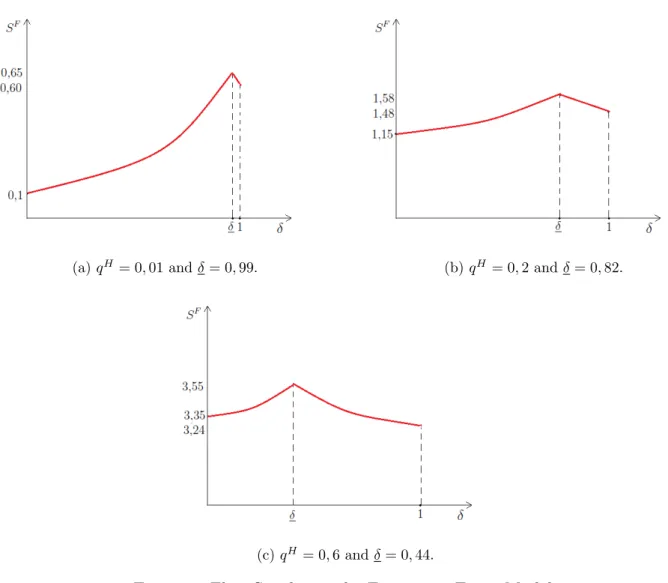
Thus, when we consider the entrance of high quality assets in the market as an exogenous variable, our flow surplus will always be maximized at exactly δ=δ.

Below we have some numerical examples of the flow surplus’ behaviour for different values of qH in a market where uH = 6, cH = 5, uL= 0,6, α= 0,5.

(a)qH _{= 0,01 andδ= 0,99. (b)q}H _{= 0,2 andδ= 0,82.}

(c)qH _{= 0,6 andδ= 0,44.}

Figure 1: Flow Surplus in the Exogenous Entry Model.

Flow Surplus in the Endogenous Entry Model

As before, when we are at type 1 equilibria we still have that increases in δ affect ˜qH

negatively and VL

1 positively. However, now we also need to take into account the additional

effects brought about by changes in qH_{. In this equilibria, we have that}

qH =GcH ₋V₁L(qH, δ)

∂qH ∂δ =−g

cH ₋V₁L(qH, δ)∂V

L

1 (qH, δ)

∂δ

h

1 +gcH ₋V₁L(qH, δ)∂V

L

1 (qH, δ)

qH

i−1

<0

What is happening here is that, as before, the increase in δ is making low type sellers more patient and thus, contributing for an increase in their reservation price. Since low quality assets become more expensive, buyers react increasing the number of offers made to potential high

quality sellers. This increase inβH will have three effects. First, it will lower the proportion of high quality assets in equilibrium, since these assets are now leaving the market faster. Secondly, it will lower the expected continuation payoff of a buyer in this market and it will increase the expected continuation payoff of the low type seller, since it will increase the probability of such seller being offered cH_{. This is where the effects of adding the agents entry decision to}

the model take place by adding a third effect: since entering the market with a low quality assets is becoming more attractive, less people will choose to pay the cost κ and the creation of high quality assets will go down. Less high quality assets entering the market will impact negatively on the buyer’s willingness to offercH_{, reducing the fall in ˜q}H _{and the growth inV}L

1 .

The end result of this effect is not very clear as it depends on the magnitude of ∂_∂δ˜qH and ∂q_∂δH, but numerical examples suggests that the latter effect is not sufficient to overcome the growth tendencies inrL

1, β1H and V1L.

Besides the indirect effects on VB

1 and V1L discussed above, we still have to account for the

direct effect of changes in qH _{on the flow surplus.}

S₁F =qHcH + (1₋qH)V₁L+V₁B

In the exogenous model we had that the liquid result of changes in VL

1 and V1B was always

positive asδ grew, but now adding the effect of changes inqH _{we can obtain different outcomes}

in terms of flow surplus. Note that even though (1₋qH_)VL

1 is still growing, now we have that

both VB

1 and qHcH are decreasing. We haven➫t been able to determine exactly when these

latter two effect overcomes the first, but we provide numerical examples to show that this is completely possible.

As δ grows and we switch from equilibria type 1 to equilibria type 2, we still find that

∂VL

2

∂δ <0, but now

qH =GcH ₋ u

L

δ

∂qH ∂δ =g

cH ₋ u

L

δ

uL

δ2 >0.

In other words, when we are at type 2 equilibria, increases in δ will rise the proportion of agents willing to enter the market with a high quality asset. The intuition behind this result is that in this equilibria, increases in δ imply a reduction in trade, impacting negatively the expected payoff of having a low quality asset in this market, thus making the idea of paying for an asset that pays dividends more attractive. This result counterbalances the negative impact

of V₂L on the flow surplus and may as well, under some conditions, outweigh it. As we can see below, the condition for increases inδto cause an increase in the flow surplus is not particularly intuitive, nevertheless it is totally possible and provides us with a major difference from the exogenous entry model.

S₂F =GcH ₋ u

L

δ

cH +h1₋GcH ₋ u

L

δ

iuL

δ ∂SF

2

∂δ =

h

GcH ₋u

L

δ

−gcH ₋u

L

δ

cH ₋u

L

δ

iuL

δ2

∂SF

2

∂δ >0⇔

h

GcH ₋ u

L

δ

−gcH ₋ u

L

δ

cH ₋ u

L

δ

i

>0

Unlike what happened with the previous model where welfare was always maximized at

δ = δ, when we incorporate the entry decision, welfare can be maximized at δ = 0, δ = ˆδ or even atδ = 1.

Given the difficulty we still have not been able to formally prove this statement, however, we show numerically that such events can really happen. First, let’s assume a functional form to our cdf G. Consider an economy where the cost one pays to transform a low quality asset into a high quality asset is distributed according to an uniform distribution with support [0, acH_],

a > _q1H. Under this assumption we have that

ˆ_δ= 1

1 + [ac

H

+(cH −uL

)+α(uH −cH

)−√[acH

+(cH −uL

)+α(uH −cH

)]2_−4acH

(cH −uL

)]α(uH −cH

) [acH_−cH_+uL_−α(uH_−cH₎₊√_[acH_+(cH_−uL_)+α(uH_−cH_)]2−4acH_(cH_−uL_)]uL

Now, consider a market where uH _{= 6, c}H _{= 5, u}L _{= 0.9, α = 0.5 and a = 2. Under}

this set up our flow surplus behaves in the same way as in the exogenous entry model and it’s maximized exactly at δ = ˆδ = 0,74.

(a) Example of Flow Surplus in the Endogenous Entry Model,ˆδ= 0,74

Under the same set up as before, but slightly decreasing a to 1,4, we now have that exact opposite situation happening. Flow surplus decreases with δ at type 1 equilibria and increases at type 2 equilibria, reaching its maximum at δ= 0.

(a) Example of Flow Surplus in the Endogenous Entry Model, ˆδ= 0,63

Finally, slightly changing uL _{from 0.9 to 0.2, we have that ˆδ = 0,22 and flow surplus is}

maximized at δ= 1.

(a) Example of Flow Surplus in the Endogenous Entry Model, ˆδ= 0,22

6

Final Remarks

In this work we have incorporated an endogenous entry of assets in a decentralized dynamic market with adverse selection. We have fully characterized the set of stationary symmetric equilibria in the model with exogenous entry and shown that each of these equilibria have a unique correspondent in the model with endogenous entry.

We found that in the latter models welfare was always maximized at the point of change between equilibria types and that, on a region where the agent’s discount rate were close enough to 1, welfare always decreased as market frictions vanished. A key difference found when incorporating the agent’s decision to create a high quality asset is that decreases in market frictions can have, on the same region withδ close enough to 1, a positive effect as they increase the incentives for the creation of such assets in a way that the amount of dividends paid by those type of assets could compensate for the fall in the gains of trade.

Due to a greater complexity of the effects in the endogenous model, we have analysed the behaviour of welfare in a very informal manner. A more rigorous approach could provide a great basis to proposed policy changes. Such analysis is left for future research.

7

References

[1] AKERLOF,G., ”The Market for ’Lemons’: Quality and the Market Mechanism,” Quar-terly Journal of Economics Studies 84 (1970), 488-500.

[2] CAMARGO, B.; LESTER,B. (2013): ”Trading Dynamics in Decentralized Markets with Adverse Selection,” mimeo.

[3] DIAMOND, P., ”A Model of Price Adjustment,” Journal of Economic Theory 3 (1971), 156-68.

[4] MORENO, D.; WOODERS, J. (2010): ”Decentralized Trade Mitigates the Lemons Problem,” International Economic Review. v.51, n.2, p.383-399.

[5] KIM,K. (2010): ”Endogenous Market Segmentation for Lemons,” mimeo.

[6] KIM,K. (2012): ”Information about Sellers’ Past Behavior in the Market for Lemons,” mimeo.

8

Appendix

Proof of Proposition 6 Consider we are in type 2 equilibrium. Since buyers are making offers that are always rejected, delaying trade is not costly, thus, V₂B = 0. Once that the buyer has a zero continuation payoff in this market, we know that rL

2 =uL (low type seller extracts

all surplus from the buyer), hence, VL

2 = u

L

δ .

When making an offer of cH_{, the buyer’s expected payoff is}

V₂B = α[˜q

H

2 (uH −cH) + (1−q˜2H)(uL−cH)

1₋(1₋α)δ = 0⇒q˜

H

2 =

cH

−uL

uH _−uL.

Now, to completely describe type 2 equilibria we need to specify the probabilities with which each price is offered and the values ofδ for which they exist. Let us use the following notation:

P r(p=cH) =σB(cH)₋σB(cH₋) =β₂H P r(p=rL) =σB(rL)₋σB(r₋L) =β₂L P r(p=p∗ < rL) = 1₋β₂H ₋β₂L

From the low type seller’s optimality and steady-state condition we have,

σL(rL)2β2L=

(1₋qH)(cH ₋uL)₋qH(uH ₋cH)

qH_(uH

−cH₎

β₂H

Note that we can only determine σL

2(rL)β2L, but we know that if an equilibrium with

σL

2(rL)<1 and β2L= ˆβ2Lexists then, an equilibrium with σL2(rL) = 1 andβ2L =σ2L(rL) ˆβ2L< β2L

will also exist. So, without loss of generality we fix σL

2(rL) = 1 and find that a necessary and

sufficient condition for this type of equilibrium to exist is

β₂H +β₂L=

(1₋qH_)(cH

−uL₎

qH_(uH

−cH₎

β₂H <1_⇔δ > u

L₍₁

−qH₎

uL₍₁

−qH_{) +αq}H₍₁

−qH₎ ≡δ

Now, consider that we are in type 1 equilibria. We know that, in this case, buyers are indifferent between offering p = cH _{and p = r}L_{, so from this indifference constraint we can}

obtain the following

˜

qH₁ uH + (1₋q˜₁H)uL₋cH = ˜q₁HδV₁B+ (1₋q˜H₁ )[σ₁L(rL)(uL₋rL) + (1₋σ₁L(rL))δV₁B]

.

Substituting the expression for VB

1 in the above equation, we have

(

1₋ αδ

1₋δ+αδ[˜q

H

1 + (1−σL1(rL))(1−q˜1H)]

)

[˜q₁HuH + (1₋q˜H₁ )uL₋cH] =σL₁(rL)(1₋q˜H₁ )[uL₋rL] (4)

Since the term between the curly brackets in left-hand side of ( 4 ) is greater than zero, we have that if ˜qH

1 > q¯H then rL1 < uL, V1B >0 and equilibria with σL(rL)1 <1 cannot exist.

Thus, type 1 equilibria withσL

1(rL)<1 may be treated as special case of type 2 equilibria with

βH

2 +β2L= 1.

We have yet to show the existence of this type of equilibria only for δ < δ. Using equa-tion ( 4), seller’s optimality and steady-state condiequa-tion one can obtain the following quadratic equation to determine ˜qH

1

∆(˜q₁H) = αδ

1₋δ+αδ[(1−δ)˜q

H

1 +αδ

qH

1₋qH(1−q˜ H

1 )][˜q1HuH + (1−q˜H1 )uL−cH]

−αδ q

H

1₋qH(1−q˜ H

1 )(u

H

−cH)₋(1₋δ)(˜q₁HuH ₋cH) = 0 (5)

Note that ∆(1) <0 and that ∆(qH) >0 _⇔ δ < δ. Ergo, equation ( 5 ) quadratic implies that, whenever δ < δ, ∆(˜qH) = 0 will have only one solution in the interval (qH,1).

Now, we are left only to prove that type 1 equilibria do not exist when δ > δ. Consider ˆ

δ= _1−q1H−q₊H_αqH > δ. Let us dived the interval (δ,1) into two smaller ones: (δ,δˆ] and (ˆδ,1).

First, note that

∆′′(˜q₁H) = 2αδ 1₋δ+αδ

1₋δ₋ αδq

H

1₋qH

(uH ₋uL)_≥0

⇔δ _≤δˆ

For the first interval it is easy to prove the non existence of a solution for ∆(˜qH_{) = 0 by}

noting that ∆(qH_{)<0, ∆(1)<0 and that ∆}′′

(˜qH₎

≥0. For the second interval, it is convenient to separate the analysis in two cases; ˜qH_uH

−cH

≤q˜H_uL _{and ˜q}H_uH

−cH _>q˜H_uL_{. In the first}

case we have,

∆(˜q₁H)<

(1₋δ)˜qH₁ +αδ q

H

1₋qH(1−q˜ H

1 )

[˜qH₁ uH + (1₋q˜₁H)uL₋cH]

−αδ q

H

1₋qH(1−q˜ H

1 )(u

H

−cH)₋(1₋δ)(˜qH₁ uH ₋cH)

= (1₋q˜H₁ )

αδqH

1₋qH −(1−δ)

[˜q₁HuH ₋cH ₋q˜₁HuL]

−αδq

H₍₁

−q˜H

1 )

1₋qH [u H

−cH ₋uL]<0

And, in the second case we have

∆(˜q₁H)<

(1₋δ)˜qH₁ +αδ q

H

1₋qH(1−q˜ H

1 )

[˜qH₁ uH + (1₋q˜₁H)uL₋cH]

−αδ q

H

1₋qH(1−q˜ H

1 )(uH −cH)−(1−δ)(˜qH1 uH −cH)

<(1₋δ)[(˜qH₁ )2uH + (1₋q˜₁H)˜q₁HuL₋q˜₁HcH ₋q˜H₁ uH +cH] = (1₋δ)(1₋q˜₁H)[˜qH₁ uL₋(˜q₁HuH ₋cH)]<0

Therefore, when δ >δˆ, ∆(˜q₁H) <0 for every ˜qH _∈ [¯qH,1) and there is no type 1 equilibria when δ > δ.

Proof of lemma 8 Fix δ. Note that δ is decreasing in qH and that when qH = 0, δ = 1. Thereby, when qH is sufficiently small,δ < δ, equilibria is of type 1 andG(VH₋VL) = G(cH). In this region, as qH increasesV₁L also increases, causing G(cH ₋V₁L) to decrease.

∂VL

1

∂qH =

αcH₍₁

−δ)(1₋q˜H

1 )˜q1H

[(1₋δ)(1₋qH_)˜qH

1 +αδqH(1−q˜1H)]2

>0

∂VL

1

∂q˜H

1

=₋ αc

H₍₁

−δ)(1₋qH_)qH

[(1₋δ)(1₋qH_)˜qH

1 +αδqH(1−q˜1H)]2

<0

∂q˜H

∂qH =− ∂∆(˜qH

1 ,δ)

∂qH

∂∆(˜qH

1 ,δ)

∂q˜H

1

<0, since

∂∆(˜qH

1 , δ)

∂qH =

αδ(1₋q˜H₎

(1₋qH₎2

h αδ

1₋δ+αδ(˜q

H

1 u

H

+ (1₋q˜H₁ )uL₋cH) +uH ₋cHi <0 and ∂∆(˜q₁H, δ)

∂q˜H <0

Eventually, with the growth of qH _{and decrease of δ, δ}

≥ δ and we will switch to type 2 equilibria where G(cH

−VL

2 ) = G(cH − u

L

δ ) is a constant. Note also, that G(c H

−VL_{) is}

continuous inqH _asG(cH

−VL

2 )

δ=δ =G(c H

−VL

1 )

δ=δ. It is easy to see thatq

H _=G(vH

−VL₎

will have one of the following formats and, thus, a unique solution, ˆqH, in [0, qH).

(a) (b) (c)

Figure 5: Different types of possible equilibria.

Now, consider that we are exactly in the case where the equilibrium occurs at the point of division between type 1 and type 2 equilibria. In this scenario, the proportion of high quality assets that enter the market will be determined by the below equation.

qH =G cH ₋ u

L

δ(qH₎

!

(6)

Note that as the left-hand side of the equation grows, δ(qH) will decrease, causing the the hand side of the equation to drop as well. As the left-hand side approaches 0, the right-hand side approaches G(cH

−uL_{)>0 and as the left-hand side approaches ¯q}H_{, the right-hand}

side approachesG(1₋α))(cH

−uL_{)< G(c}H_)<q¯H_{. Given that, it is easy to see that equation}

( 6 ) has an unique solution, qH _{= q}H_{, meaning that equilibria as that of case (b) in Figure 5}

will only happen when δ=δ(qH₎

≡ˆδ.

At the point of division between both equilibria type it’s always true that VL

1 = V2L and

˜

qH _=qH_{. From these conditions we can obtain an equation for q}H _{as a function of δ.}

qH = u

L₍₁

−δ)

uL₍₁

−δ) +αδ(uH

−cH₎ (7)

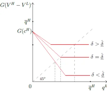
Now, note that if δ increases to δ > ˆδ, the constant part of G(VH ₋VL) graph will shift up and to the left, causing equilibria to be of type 2. If the opposite occurs, the constant part

G(cH

− uδL) will shift down and to the right inducing equilibria to be of type 1, as the figure

below shows.

Figure 6: Equilibria for different values of δ.

Flow Surplus in the Exogenous Entry Model

V₁B = α[β

H

1 (˜q1HuH + (1−q˜1H)uL−cH) + (1−β1H)(1−q˜1H)(uL−r1L)]

1₋(1₋α)δ₋(1₋βH

1 )αδq˜1H

Using the fact that ˜qH = _(1−qHqH

)βH

+qH and that the buyer is indifferent between offeringc

H

orrL

1 we have:

V₁B = α[˜q

H

1 uH + (1−q˜1H)uL−cH]

(1₋δ)[(1₋qH_)βH _+qH_{] +αδβ}H

∂VB

1

∂βH ∝ −[(1−δ) (1−q

H_)βH _+qH

+αδβH][α(1₋qH)(cH ₋uL)]

−α[(1₋δ)(1₋qH) +αδ][qH(uH ₋cH) + (1₋qH)βH(uL₋cH)]<0

V₁L= αβ

H

1 cH

1₋(1₋αβH_)δ

∂VL

1

∂δ ∝[1−δ+αδβ

H

]

αcH∂β

H

∂δ

−αβHcH

−1 +αβH +αδ∂β

H

∂δ

=αβHcH(1₋αβH) + (1₋δ)αcH∂β

H

∂δ >0