Price discovery using a regime-sensitive cointegration approach

(1)

FUNDAÇÃO GETULIO VARGAS ESCOLA DE ECONOMIA DE SÃO PAULO

EDUARDO MATHIAS HINTERHOLZ

PRICE DISCOVERY USING A REGIME-SENSITIVE

COINTEGRATION APPROACH

(2)

PRICE DISCOVERY USING A REGIME-SENSITIVE

COINTEGRATION APPROACH

Dissertação apresentada à Escola de Economia de São Paulo da Fundação Getulio Vargas, como requisito para obtenção do título de Mestre em Economia

Campo de Conhecimento: Finanças Empíricas

Orientador: Prof. Dr. Pedro Luiz Valls Pereira

(3)

(4)

PRICE DISCOVERY USING A REGIME-SENSITIVE

COINTEGRATION APPROACH

Dissertação apresentada à Escola de Economia de São Paulo da Fundação Getulio Vargas, como requisito para obtenção do título de Mestre em Economia

Campo de Conhecimento: Econometria de Finanças

Orientador: Prof. Dr. Pedro Luiz Valls Pereira

Data de Aprovação:

/ /

Banca examinadora:

Prof. Dr. Pedro Luiz Valls Pereira (Orientador)

FGV - EESP

Prof. Dr. Marcelo Fernandes FGV-EESP e Queen Mary University of

London

(5)

Agradecimentos

Em primeiro lugar agradeço à minha família por me incentivarem e me apoiarem incondi-cionalmente.

Agradeço à minha turma de mestrado pelo grande companheirismo: foi essencial a con-vivência com vocês neste ambiente desaﬁador em que todos foram muito colaborativos. Não menos importantes foram as turmas anteriores e o pessoal do CEQEF. Obrigado pela grande amizade e aconselhamentos.

Também sou grato pela segunda família que encontrei em São Paulo. Com o Momo, Cenci e Mexicano tive muitas alegrias, estudos e aprendizados que levarei pela vida.

Meu muito obrigado aos professores da banca pelos valiosos conselhos. Em especial ao pro-fessor Marcelo Fernandes, o qual sempre esteve disponível para dúvidas e aconselhamentos durante a confecção deste trabalho.

Não posso deixar de agradecer ao professor Eduardo Mendes pelos conselhos, tempo e auxílio em econometria Bayesiana.

(6)

ABSTRACT

This work proposes a method to examine variations in the cointegration relation between preferred and common stocks in the Brazilian stock market via Markovian regime switches. It aims on contributing for future works in "pairs trading" and, more specifically, to price discovery, given that, conditional on the state, the system is assumed stationary. This implies there exists a (conditional) moving average representation from which measures of "informa-tion share" (IS) could be extracted. For identifica"informa-tion purposes, the Markov error correc"informa-tion model is estimated within a Bayesian MCMC framework. Inference and capability of detect-ing regime changes are shown usdetect-ing a Montecarlo experiment. I also highlight the necessity of modeling financial effects of high frequency data for reliable inference.

(7)

RESUMO

Este trabalho propõe um método para examinar variações na relação cointegração de preços de ações preferenciais e ordinárias da bolsa brasileira através de mudanças de regime no sentido de Markov. Este modelo tem como objetivo contribuir tanto para futuros tra-balhos em negociações de pares ("pairs trading") quanto, principalmente, para aplicação em descoberta de preços visto que, condicional nos estados, é pressuposta estacionariedade no sistema. Desta maneira seria possível a extração de medidas de "parcela de informação" (IS) baseadas na representação de médias móveis de um modelo de correção de erros Markoviano, estimado através de um ferramental bayesiano do tipo MCMC por questões de identiﬁcação. A validade do modelo no sentido de capturar as variações de regime é demonstrada através de experimento de Montecarlo, bem como é evidenciada a necessidade da modelar não nor-malidades na distribuição dos dados de alta frequência visando inferência.

(8)

1 Introduction

The modeling of long run stable relations has always been key to the economics literature. The theorem of representation by Engle e Granger (1987) allowed the study of non-stationary time series built on this very principle. In particular, a large part of the academia interested in ﬁnance (and ﬁnancial econometrics) has been devoting great attention to understand the joint evolution of asset prices.

In recent years there has been a signiﬁcant increase of available data and high frequency traders have been pivotal to a more rigorous assessment of the dynamics of information dis-semination among markets.

Price discovery relies on the fundamental value of the firms. For illustration, if we look at the prices of two different classes of the same stock (say PETR4 and PETR3, for Brazil-ian oil company Petrobras preferred and common shares respectively) no arbitrage tells us we must not have strong divergences on their patterns. This implies that they eventually cointegrate. The question that arises is then which share class reacts first to the arrival of relevant information.

The methodological contribution in Fernandes e Scherrer (2012) propose a measure of Information Share (IS) based on the relative variance of the innovations vector of the moving average (VMA) representation of the error correction process. The authors, however, suggest that this measure is not constant over the whole period considered in the paper.

This opens a window of possibilities for considering non-linear models. In particular, the results in Granger e Siklos (1997), who argue that there’s no reason to expect the error cor-rection process to be symmetric and linear, are explored by allowing the equilibrium relation between the price series to be temporarily "switched oﬀ". If this is the case, there exists two VMA representations of the system, which can give rise to two IS measures.

In their paper, however, the exact moment when the structural break point occurs is com-pletely exogenous. Psaradakis, Sola e Spagnolo (2004) extend the idea by introducing a Markov error correction (MEC) model where the changes of regime are produced endoge-nously. To detect this behavior they use a multi-step test procedure as in Balke e Fomby (1997), which looks at diﬀerences between local and global evolution of the system1_.

1

(10)

Chapter 1. Introduction 10

Although valid, threshold cointegration as in Balke e Fomby (1997) is potentially mislead-ing either in small samples or if the regime where cointegration is present is not the dominant over the period, as pointed out by Sugita (2008). To circumvent these issues, I follow the methodology in Sugita (2006) by employing a Bayesian technique, which circumvents identi-ﬁcation and inference issues in estimating the VECM.

This setup is then applied to high frequency ﬁnancial data in the Brazilian stock market. Particularly, I’m interested in the dual-class eﬀects of information dissemination as investi-gated in Fernandes e Scherrer (2012). I restrict attention to the two companies with most liquid stocks in the local market and asses the capability of the model in identifying a Marko-vian error correction model.

(11)

11

2 Data

The database is constructed using tick by tick transaction information from B&MFBOVESPA (the Brazilian stock exchange) for Petrobras (Petróleo Brasileiro S.A.) and Vale from January 2011 through December 2011.

In the Brazilian market, Petrobras and Vale issue two types of shares: common (or ON -PETR3 and VALE3 respectively) and preferred (or PN - PETR4 and VALE5 respectively). Due to regulatory issues, until January 2001 all national companies listed in the local stock exchange were allowed a 2-by-1 issuance rate for PN:ON, leaving a ratio of shares outstanding of about 3-to-1 as of today. This has great impact on liquidity diﬀerences, which will force gathering data at a high frequency in order not to distort any lead-lag eﬀect1_.

Regular trading (excluding pre and after-market) hours in Bovespa range from 10:00:00 AM to 5:00:00 PM from mid February until mid November. The rest of the year accounts for "daylight saving time", in which trading hours are delayed by one hour. Despite the vast amount of information on each tick, only transaction prices (in logarithm) are kept.

2.1 Data filtering

Dealing with tick data raises concerns about the quality of the information contained. As stated by Brownlees e Gallo (2006), the faster the trades occur the greater the chances of noise2 _{in data.}

In what follows, I adopt the methodology in Brownlees e Gallo (2006) which is, for conve-nience, described below:

1. Set i=1 and letpi denote the "ith" available price of a day in sample

2. Construct ¯pi(k, δ) and si(k, δ), the δ trimmed mean and standard deviation in the

vicinity of k observations3 _around_p

i

1

Suppose stocks A and B are traded and A is more liquid. If we aggregate in a sufficiently low frequency we can’t observe stock B only responding seconds later to a variation in A

2

Bid-ask bounce, wrong reporting and market inconsistent quotes are examples

3

(12)

Chapter 2. Data 12

3. If |pi −p¯i(k, δ)|< 3si(k, δ) +γ, where γ is a granularity parameter, we keep pi. Else,

pi is discarded.

4. Set i=i+1 and repeat items 2-4 until i=N, the number of transactions for each security. Before running the above steps I also discard the ﬁrst and last 15 minutes of trades of the day. This is done to disregard opening and closing market activities which, in general, account for greater trading intensity.

Table 2.1.1 reports raw data count and quantity of trades after ﬁltering, for each security. Percentage of outliers is also informed.

According to the literature, the filtering procedure is quite sensitive to the choice of k and γ. It is good practice to choose k according to the securities’ liquidity, so that the time span covered by the window is not too large, which could cause outliers to be misidentified. In this work k is allowed to vary with trade intensity, ranging from 30 (for less liquid periods) to 60. The granularity parameter is fixed at 0.01, the smallest possible price variation, guaranteeing|pi−p¯i(k, δ)|= 0< γ whenever si(k, δ) = 0.

Table 2.1.1 shows the number of transactions before and after ﬁltering, as well as the percentage of outliers detected by the algorithm.

Table 2.1.1 – Raw and ﬁltered data for δ = 10% reported in millions of observations Company Ticker # of Raw Observations # of Filtered Observations Outliers (%)

Petrobras PETR4 5.664 5.216 7.91

Petrobras PETR3 2.084 1.947 6.60

Vale VALE5 5.237 4.810 8.15

Vale VALE3 2.047 1.906 6.92

2.2 Data aggregation

In order to adopt the methodology in Fernandes e Scherrer (2012) one must have equally spaced observations. To do so I consider time windows of 5 and 15 minutes (giving rise to roughly 78 and 26 observations respectively per day). The "window price" is chosen such that synchronicity is respected. This goal is achieved by minimizing the diﬀerence in time when transactions occur4 _{which also attenuates the eﬀects of the lack of liquidity of the local}

4

(13)

market.

Empty windows have its price repeated from the previous observation5_.

Aggregation plays a role since it represents an important trade-oﬀ: the lower the frequency, the lower the contemporaneous correlation but also the lower the microstructure eﬀects.

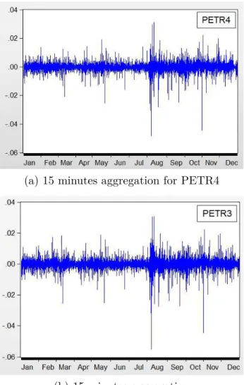
Figures 1 and 2 plot the returns for Petrobras in 5 and 15 aggregation intervals. The plots suggest non-constant oscillatory behavior through the year, with periods of higher variation. The shock in the beginning of august appears to be of major importance and persistence. Figure 1 – Returns for Petrobras: 5 minutes aggregation intervals. y axis represents returns

in decimals

(a) 5 minutes aggregation for PETR4

(b) 5 minutes aggregation for PETR3

5

(14)

Figure 2 – Returns for Petrobras: 15 minutes aggregation intervals. y axis represents returns in decimals

(a) 15 minutes aggregation for PETR4

(b) 15 minutes aggregation

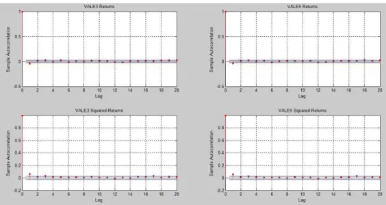
To examine the persistent behavior I look at the autocorrelation of the returns and squared-returns in ﬁgure6 _{3. For both PETR3 and PETR4 the eﬀects of the lagged}

re-turns on their contemporary counterpart appear statistically insigniﬁcant after 3 lags. The same inference, however, can’t be drawn if looking at the squared returns, which can be an indicative of strong variance persistence.

6

(15)

Figure 3 – Autocorrelations for Petrobras

(16)

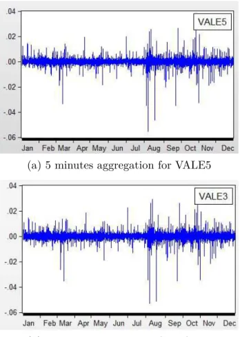
Figure 4 – Returns for Vale: 5 minutes aggregation intervals. y axis represents returns in decimals

(a) 5 minutes aggregation for VALE5

(17)

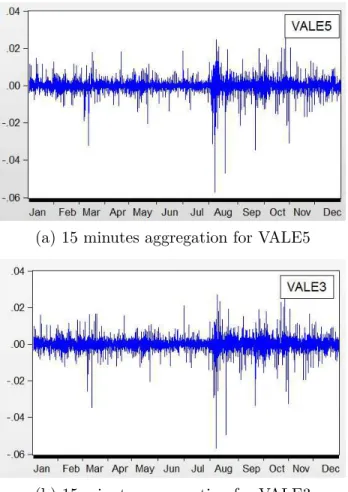
Figure 5 – Returns for Vale: 15 minutes aggregation intervals. y axis represents returns in decimals

(a) 15 minutes aggregation for VALE5

(b) 15 minutes aggregation for VALE3

(18)

Figure 6 – Autocorrelations for Vale

A quick visual inspection would suggest that the returns and squared-returns for Vale are more short-lived if compared to the returns of the oil company.

In general, 2011 can be considered turbulent in the ﬁnancial markets, being not much favorable to emerging markets.

In early march, a nuclear catastrophe in Japan plummeted commodities prices, adding more volatility to asset prices. In particular Vale was mostly aﬀected, having Japan as an im-portant commercial partner, with exports to that country representing around 11% of whole exports in 2010.

By the end of may of 2011 the European Union oﬀers ﬁnancial support for Portugal and Ireland, while Greece struggles to repay its debts.

August is marked as critical month due to contagion risk in Europe. The lack of resolution of this sovereign situation causes a lack of liquidity of the global financial system on the second semester. Combined with a weak demand of the G3 countries, slowing Chinese growth and a drop in the business confidence in Brazil, the second semester is also marked as very volatile in the financial market.

(19)

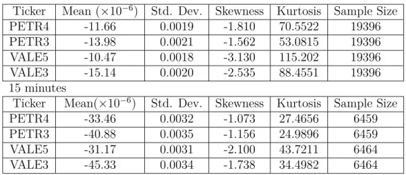
Table 2.2.1 – Descriptive statistics of returns for aggregation intervals 5 minutes

Ticker Mean (×10−6_{) Std. Dev. Skewness Kurtosis Sample Size}

PETR4 -11.66 0.0019 -1.810 70.5522 19396

PETR3 -13.98 0.0021 -1.562 53.0815 19396

VALE5 -10.47 0.0018 -3.130 115.202 19396

VALE3 -15.14 0.0020 -2.535 88.4551 19396

15 minutes

Ticker Mean(×10−6₎ _{Std. Dev. Skewness Kurtosis Sample Size}

PETR4 -33.46 0.0032 -1.073 27.4656 6459

PETR3 -40.88 0.0035 -1.156 24.9896 6459

VALE5 -31.17 0.0031 -2.100 43.7211 6464

VALE3 -45.33 0.0034 -1.738 34.4982 6464

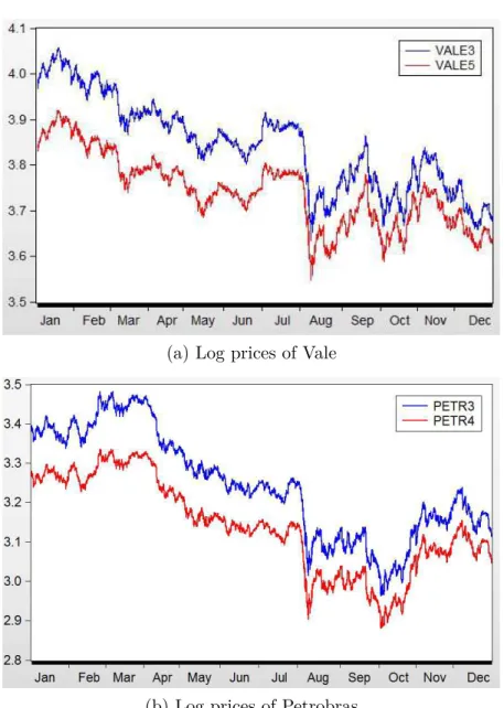
Figure 7 plots the logarithm of the prices for Petrobras and Vale with a 5 minute ag-gregation window7_{. From January until the beginning of August there’s a clear downward}

trend which may be explained by internally by weak industrial production and a tightening monetary cicle and globally by uncertainties regarding the contagion risk of the European debt crisis8_{. For the rest of the year there exists a noticeable rebound by the end of August}

that lost force, which can be related to the lack of global liquidity and slow economic recovery of Europe, China and USA, making the performance of the preferred shares of Petrobras and Vale close the year with a negative return of approximately 20.2% and 25.8% respectively and the common stocks with losses around 23.1% and 28.4% in the period.

7

15 minute aggregation won’t be plotted due to the great similarity of the series in level.

8

(20)

Figure 7 – Log prices in 5 minutes aggregation

(a) Log prices of Vale

(21)

21

3 The Model

3.1 Markov Switching Error Correction Model

Consider {xi

t}Tt=1 to be, for each i ∈ I ≡ {1, ..., N}, an integrated of order 1 time series

and, for sake of notation, deﬁneXt ≡ [x1t ... xNt ]′. Assume there exists a set of r vectors

β ∈ RN _×_Rr _{for which} _β′_X

t with t ∈ T ⊂ {1,2, ..., T} is a vector with stationary time

series (in any other subset of times they do not cointegrate).

Let St follow a ﬁrst-order two states Markov chain with transition probabilities (pii, pjj)

with i, j ∈S_{≡ {0,}_1} _and _i₆₌_{j, i.e.,} _S_t_∈S _∀t_∈_1,_{2, ...T} _and _{∀i, j} _∈S_, Prob(St =j|St−1 =i) =pij .

If we assumet∈T _iﬀ _S_t _{= 1 we might want to jointly model these time series using a} vector error correction representation with Markov switching behavior:

∆Xt=µ+α(St)β′Xt−1+

p−1

X

i=1

Φi∆Xt−i+εt (3.1)

with εt ∼ N(0,Σ(St)), µ being a constant parameter and α(St) an Nxr matrix of loadings

that evolves according to the Markovian process above.

To cope with the setup in Sugita (2006) I also allow the constant term µ and the lagged variable coeﬃcients Φ to be regime-dependent. Hence, equation 3.1 could be conveniently rewritten as:

∆Xt=µ(St) +α(St)β′Xt−1+

p−1

X

i=1

Φi(St)∆Xt−i+εt (3.2)

Notice that equation 3.2 has a natural matrix representation of the form:

Y =XΓ +Zβα′+E ≡W B+E (3.3)

with W = [X I0Zβ I1Zβ] and B = [Γ′ α]′, α= [α1, α0],

(22)

Chapter 3. The Model 22 Y =         ∆X′ p ∆X′ p+1 ... ∆XT        

, Z =

        X′ p−1 X′ p ... XT−1

       

, E =

        ε′ p ε′ p+1 ... ε′ T         X=        

s1,p s0,p s1,p∆Xp′−1 . . . s1,p∆X1′ s0,p∆Xp′−1 . . . s0,p∆X1′

s1,p+1 s0,p+1 s1,p+1∆Xp′ . . . s1,p+1∆X2′ s0,p+1∆Xp′ . . . s1,p+1∆X2′

... ... ... . . . ... ... ... ...

s1,T s0,T s1,T∆XT′−1 . . . s1,T∆XT′−p+1 s0,T∆XT′−1 . . . s0,T∆XT′−p+1

       

As in Sugita (2006) sm,t is an indicator variable 1{St = m} and Im is a square matrix

where the oﬀ-diagonal elements are equal to 0 and the t-th diagonal entry issm,t.

3.2 Estimation

Testing for breaks in the cointegration relation using classical methods is an intricate problem. In particular, consider the hypothesis test (in usual notation) on equation 3.2:

T :







H0 : α(St) = 0

H1 : α(St) 6= 0

It is clear that the model is not identified under the null. Andrews e Ploberger (1994), for example, offer a theoretical framework for testing for breakpoints under non identifiability of nuisance parameters. Some ex ante structure, however, must be assumed for detection. Balke e Fomby (1997) propose a multi-step algorithm in which they detect global cointegration and test locally for parameter instability and non-linearities, building thresholds for the long run relation. Given the lack of power of Johansen’s tests under non-normality of the residual, this alternative could be potentially misleading.

In a Bayesian framework, however, those problems do not arise: nuisance parameters are integrated out of the joint conditional probability distribution and testing for changes in regime becomes an issue of model selection using Bayes factors. Throughout, β is assumed to be known and r is kept ﬁxed and equal to 1.

With this in mind, this work employs a Gibbs-Sampling strategy as follows: 1. Set i=1 and give starting values ˜ST(0) ={S

(0) 1 , S

(0) 2 , ..., S

(0)

(23)

Chapter 3. The Model 23

2. Generate B(i) _from_p(B|β,_Σ(i−1)_,_S˜(i−1)

T , Y) and Σ(mi) fromp(Σm|B(i),S˜( i−1)

T , Y) ;

3. Generate (p00, p11)(i) fromp(p00, p11|S˜(

i−1)

T );

4. Generate ˜ST(i) fromp( ˜S

(i−1)

T |Θ(i), Y), where Θ ={B,Σm, p00, p11}, using the multi-move

Gibbbs Sampling (forward ﬁltering, backward sampling); 5. Set i=i+1 and go back to 2.

where p(Ξ|η) denotes the posterior distribution of Ξ conditional on η, for any two random variables (Ξ, η).

3.2.1 Identification restrictions

The Gibbs sampling algorithm is not able to identify neither the state variables nor the transition probabilities if the true data generating process in not regime dependent. For this reason I follow the methodology in Koop e Potter (1999) and restrict,a priori, that each state occurs at least 15% and at most 85% of the time at the states vector ˜ST. That is, for state m,

15≤

τ

X

t=1

sm,t/τ ≤85%

If this restriction is not satisﬁed at any run i of the Gibbs sampler make ˜ST(i) = ˜S

(i−1)

T .

3.2.2 Priors, posteriors and sampling scheme

Inference on equation 3.3 requires no speciﬁc structures for priors, i.e., they are allowed to be diﬀuse (except for the cointegrating vector). However, the computation of Bayes factors require them to be proper. Following Sugita (2006), priors are chosen as:

Σm ∼IW(Sm, hm)

vec(B)∼M N(P,ΩB)

p00 ∼beta(u00, u01)

p11 ∼beta(u11, u10)

(3.4)

where IW and MN stand for the inverse wishart and matrix normal distributions respectively, S has the same dimensions of Σm, hm represents degrees of freedom in IW,P the mean of

(24)

Chapter 3. The Model 24

This formulation also implies prior independence between Σm and B, i.e.:

p(B|Σ1,Σ0) =p(B)p(Σ1,Σ0)

The posterior distributions are all derived in Sugita (2006)1 _{and result in:}

Σm|B,S˜T, Y ∼IW([Ym−WmB]′[Ym−WmB] +Sm, hm+τm)

p00|S˜T, Y ∼beta(u00+m00, u01+m01)

p11S˜T, Y ∼beta(u11+m11, u10+m10)

vec(B)|Σm,S˜T, Y ∼M N(vec(B∗), M∗)

(3.5)

withmij representing the number of transitions from state i to state j andτm = τ

P

t=1sm,t. Also:

M∗ =

( Ω−1 B + 1 X m=0 [Σ−1

m ⊗(W

′

mWm)]

)−1

and

vec(B∗) =M∗

(

Ω−1

B P +

1

X

m=0

[(Σ−1

m ⊗I)vec(W

′

mYm)]

)

To sample from ˜ST the choice is made for the multi-move Gibbs sampler. A forward

ﬁltering is performed based on Hamilton (1989) and backward sampling from the relation:

Pr(St= 1|St+1, Y,Θ) =

Pr(St+1|St = 1)Pr(St = 1|Θ, Y)

P1

j=0pr(St+1|St=j)Pr(St=j|Θ, Y)

(3.6) for t=T-1,T-2...1.

Once equation 3.6 is computed, letube a realization ofU ∼U[0,1], the uniform distribution.

Set St= 1 if Pr(St= 1|St+1, Y,Θ)≥u and 0 if contrary.

1

(25)

25

4 Montecarlo experiment and application

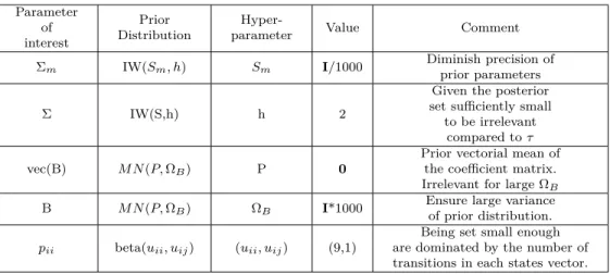
The upcoming sections are devoted to testing and implementing the model. For this purpose, the hyperparameters used in the prior distributions were chosen considering com-plete unawareness about the true parameter values. Table 4.0.1 brieﬂy discusses each of the arguments1_:

Table 4.0.1 – Prior Hyperparameters

Parameter of interest Prior Distribution

Hyper-parameter Value Comment

Σm IW(Sm, h) Sm I/1000 Diminish precision of

prior parameters

Σ IW(S,h) h 2

Given the posterior set sufficiently small to be irrelevant

compared toτ

vec(B) M N(P,ΩB) P 0

Prior vectorial mean of the coefficient matrix. Irrelevant for large ΩB

B M N(P,ΩB) ΩB I*1000 Ensure large variance_{of prior distribution.}

pii beta(uii, uij) (uii, uij) (9,1)

Being set small enough are dominated by the number of transitions in each states vector. Note:i, j= 0,1 andi6=jin the last line of the table.

Except for the prior hyperparameters of the transition probabilities’ distributions2 _the

following exercises were performed with diﬀerent prior parameters to insure robustness. As desired (and also pointed by Sugita (2008)), these choices have no impact on model inference.

1

Dimensions omitted.

2

(26)

Chapter 4. Montecarlo experiment and application 26

4.1 Artificial data

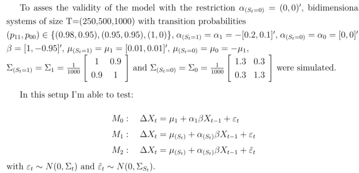
To asses the validity of the model with the restriction α(St=0) = (0,0)

′_{, bidimensional}

systems of size T=(250,500,1000) with transition probabilities

(p11, p00)∈ {(0.98,0.95),(0.95,0.95),(1,0)},α(St=1)=α1 =−[0.2,0.1]

′_,_α

(St=0) =α0 = [0,0]

′_,

β= [1,−0.95]′_, _µ

(St=1) =µ1 = [0.01,0.01]

′_, _µ

(St=0) =µ0 =−µ1,

Σ(St=1) = Σ1 =

1 1000   1 0.9 0.9 1 

and Σ₍_S_t₌₀₎ = Σ₀ = 1

1000   1.3 0.3 0.3 1.3 

were simulated.

In this setup I’m able to test:

M0 : ∆Xt =µ1+α1βXt−1+εt

M1 : ∆Xt =µ(St)+α(St)βXt−1 +εt

M2 : ∆Xt =µ(St)+α(St)βXt−1 + ˜εt

with εt∼N(0,Σt) and ˜εt ∼N(0,ΣSt).

Table 4.1.1 shows the means, standard deviations and high frequency intervals of the sampled posterior distributions with size T=1000 and (p11, p00) = (0.98,0.95) .

For the rest of the set of tested probabilities we see that all of the parameters lie inside a 95% frequency interval. Appendix B shows the results for generated models with T=500 and T=250. In general lines, smaller sample sizes tend to generate wider probability density intervals for the estimates, which also contain the true parameter values.

To save space, results for (p11, p00) = (0.95,0.95) are not reported and are available upon

request 3_.

3

Notice that (p11, p00) = (1,0) is not identified under models M1 and M2, although a qualitative result

(27)

Table 4.1.1 – Parameter estimates using Bayesian framework with 30,000 iterations and burn-in period of 10,000. Abusburn-ing notation, subscript i burn-in µmi represents the i-th

entry of the vector µ(St =m). Same is true for αi, which will be reported only

for m = 1 since it is ﬁxed otherwise. True model: M2

Parameter True value Mean Median Std. Dev. 95% HFI

α1 -0.2 -0.2044 -0.2041 0.0322 [-0.2674, -0.1421]

α2 -0.1 -0.1097 -0.1095 0.0300 [-0.1697, -0.0514]

µ01 -0.01 -0.0069 -0.0069 0.0024 [-0.0118, -0.0020]

µ02 -0.01 -0.0085 -0.0085 0.0026 [-0.0138, -0.0031]

µ11 0.01 0.01102 0.01101 0.0012 [0.00859, 0.01351]

µ12 0.01 0.01055 0.01055 0.0012 [0.00325, 0.01292]

p00 0.95 0.93556 0.9375 0.0193 [0.8925, 0.9697]

p11 0.98 0.97747 0.9784 0.0066 [0.9630, 0.9888]

|Σ1|= det





0.0010 8.6122e−04 8.6122e−04 9.2464e−04



= 1.8909e−07,

|Σ2|= det





0.0011 2.079e−04 2.079e−04 0.0013



= 1.4733e−07.

Figure 8 shows smoothed probabilities P(St = 1|Y) plotted against the generated state

vector ˜ST, indicating good performance in identifying Markovian states.

Figure 8 – Smoothed probabilities (blue line) capturing the true generated state vector (red dots)

Posterior probability for M2 when the true model is M2 generated with T=1000 (when

(28)

selection via Bayes factors (approximated by BIC Shwarz Criteria) is sensitive to sample size, being more able to capture non-linearities in the data as it increases.

4.1.1 MCMC diagnostics

Tables 4.1.2, 4.1.3, 4.1.4 and 4.1.5 report eﬀective sample size and convergence diagnostics by Geweke (1992), Heidelberger e Welch (1983), Raftery e Lewis (1992) and Raftery e Lewis (1995) respectively.

Table 4.1.2 shows the number of eﬀectively independent draws generated by the MCMC simulation for each parameter, after burn-in. It is a measure of sample size corrected by the autocorrelation in the chain.

Table 4.1.2 – Eﬀective chain size after correcting for autocorrelation. 20,000 iterations after burn-in

Parameter Eﬀective Size α1 16,713.306

α2 16,284.565

µ01 14,621.949

µ02 14,057.290

µ11 16,763.774

µ12 16,513.425

p00 8,241.985

p11 7,811.379

it indicates fairly good mixing of the chains, even for the transition probabilities.

(29)

Table 4.1.3 – Geweke diagnostic: comparing means of the first 10% and last 50% of the chain. The proposed statistic is constructed on the difference of the means and has asymptotic standard normal distribution. Tested at a 5% significance level.

Parameter Statistic Diagnostic α1 -1.5186 Equal

α2 -1.4579 Equal

µ01 -1.4541 Equal

µ02 -0.4264 Equal

µ11 0.4480 Equal

µ12 0.4899 Equal

p00 1.7713 Equal

p11 0.4274 Equal

Table 4.1.4 reinforces the results found in Geweke’s test. Its diagnostics are based on a two step procedure:

• In step 1 a Cramer-von-Mises statistics is employed to test the null of stationarity of the sample. It is done ﬁrstly on the whole sample and then successively discarding the ﬁrst 10% until the null is accepted or half of the sample is discarded. If the test is passed (null accepted), we move to the next step.

• Half of the width of a conﬁdence interval is calculated using the part of the sample not discarded in the previous step. If the ratio of the mean over the "halfwidth" measure is suﬃciently small, the test is passed, indicating stationarity.

Table 4.1.4 – Heidelberg and Welch diagnosis: a two step stationarity test Parameter p-Value Stationarity result Halfwidth result

α1 0.0929 Passed Passed

α2 0.0640 Passed Passed

µ01 0.2504 Passed Passed

p00 0.1679 Passed Passed

p11 0.8847 Passed Passed

(30)

distribution given, an acceptance tolerance. Then it runs a pilot sampler and suggests the number of iterations necessary to achieve convergence, a burn-in period and a dependence factor, which can be interpreted as a proportional increase in the number of iterations nec-essary due to chain autocorrelation. Base on these criteria the whole set of parameters seem to have been well generated by the employed algorithm.

Table 4.1.5 – Raftery-Lewis diagnostics with quantile = 0.025, accuracy = ±5×10−3 _and

95% probability

Parameter Burn-in(M) Total iterations (N) Integrating/Dependence Factor

α1 2 3,746 1.03

α2 2 3,746 1.02

µ01 2 3,746 1.01

µ02 3 3,746 1.07

µ11 2 3,746 1.02

µ12 2 3,746 1.03

p00 4 3,746 1.33

p11 4 3,746 1.31

Altogether with a visual inspection of the autocorrelation plots in ﬁgure 11 (see appendix A) and the results in this section one can conclude that this model is able to capture the Markov switching behavior of a two states error correction model and sample the parameters reasonably well, delivering good convergence results.

4.2 Tick-by-tick aggregated transaction prices

As can be noticed, the distribution of the returns of the stocks present a very elevated kurtosis. Also, there appears to be some persistence of squared the stocks in study.

This is troublesome in this framework: assuming identification restrictions as in Koop e Pot-ter (1999), the states vector is repeated more than 99% of the times of the Gibbs sampling iterations, resulting in lack of identification of the parameters. For sake of illustration, figure 9 shows the first 1000 iterations of the algorithm for Petrobras in 15 minutes aggregation intervals when sampling the vector µ1. It turns out that this is the same output delivered

(31)

Figure 9 – Problematic sampling for Petrobras

Looking at figure 10, it suggests that there exists a possible regime dependent α that is different from (0,0) in both states. To give this extra flexibility for the model I let α0 be

jointly estimated in B. The same behavior as above is reached and the algorithm is stopped. A very similar characteristic is presented when running the model for Vale, either restricting the loading parameter or not.

Figure 10 – Dispersion plots for Petrobras

A visual inspection of ﬁgure 7, however, clearly suggests a long run relation between common and preferred stocks.

(32)

32

5 Conclusion

The theoretical contributions of Fernandes e Scherrer (2012) came as a turning point on the evaluation of information shares, in the sense of simplicity and robustness. Also their ﬁndings about its non constancy during periods of market distress opened a front of research for modeling the high frequency data using a Markov switching framework.

Building on those results this paper looks at the model proposed by Sugita (2006), which circumvents issues of non identiﬁability and inference that arise in standard likelihood-based methods and applies to the Brazilian ﬁnancial market context, using Petrobras’ and Vale’s common and preferred stocks traded at BM&FBOVESPA.

Great care with data handling, however, is crucial for working within this framework since stationarity is assumed at each given state: presence of too much noise might well invalidate the model.

As seen in the simulated exercise, the Bayesian strategy seems to well identify the Markov Switching behavior of the series. By marginally modifying the model in Sugita (2006) great convergence results are obtained using Montecarlo simulations.

Dealing with high frequency data, however, exacerbates stylized facts of ﬁnancial time series1_{. In particular, the presence of kurtosis and persistent heteroskedastic behavior in the}

distribution of the returns may well undermine Johansen’s test due to a lack of power. It turns out that these characteristics also bring difficulties on the identification of the nuisance parameters under the presented Bayesian framework. Indeed, the chosen sample present characteristics that undermine identification and convergence of the proposed model.

Future work might want to devote special attention to such eﬀects by imposing a more ﬂexible structure for the variance/covariance matrix. Additionally, Koop, Leon-Gonzalez e Strachan (2011) propose a model where the whole cointegration space2_{evolves through time,}

which could be more adequate to the context.

1

See Tsay (2010) for reference.

2

(33)

33

A MCMC autocorrelation plots

This section is devoted for a visual inspection on the autocorrelation generated by the sampling scheme employed in section 4, with 20 thousand iterations left after discarding the ﬁrst 10 thousand as burn-in period. Interpretation of the results is given in chapter 4, together with other standard MCMC diagnostics.

A.1 Montecarlo experiment

(34)

34

B Bayesian estimates with different sample

sizes

Table B.0.1 show posterior distribution characteristics of simulated data under modelM2

for sample size T=500 and T=250 respectively. Interpretation is given in chapter 4.

Table B.0.1 – Parameter estimates with T=500 Parameter True value Mean Median Std. Dev. 95% HFI

α1 -0.2 -0.2157 -0.2041 0.0360 [-0.2866, -0.1463]

α2 -0.1 -0.1315 -0.1095 0.0348 [-0.1995, -0.0633]

µ01 -0.01 -0.0080 -0.0079 0.0033 [-0.0145, -0.00149]

µ02 -0.01 -0.0088 -0.0088 0.0034 [-0.0138, -0.0031]

µ11 0.01 0.00946 0.00944 0.0017 [0.0061, 0.01286]

µ12 0.01 0.00995 0.00994 0.0016 [0.0067, 0.01323]

p00 0.95 0.95017 0.95281 0.0020 [0.9042, 0.9814]

p11 0.98 0.98157 0.98258 0.0075 [0.9644, 0.9933]

|Σ1|= det





9.9211e−04 8.6018e−04 8.6018e−04 9.4305e−04



= 1.9569e−07,

|Σ2|= det





0.0013 4.0161e−04 4.0161e−04 0.0012



(35)

Appendix B. Bayesian estimates with different sample sizes 35

Table B.0.2 – Parameter estimates with T=500 Parameter True value Mean Median Std. Dev. 95% HFI

α1 -0.2 -0.1806 -0.1802 0.0342 [-0.2485, -0.1142]

α2 -0.1 -0.1141 -0.1139 0.0315 [-0.1766, -0.0524]

µ01 -0.01 -0.0100 -0.0100 0.0037 [-0.0174, -0.0026]

µ02 -0.01 -0.0121 -0.0121 0.0039 [-0.0199, -0.0045]

µ11 0.01 0.00680 0.00682 0.0029 [0.00010, 0.01257]

µ12 0.01 0.00548 0.00549 0.0027 [3.0e-05, 0.01088]

p00 0.95 0.96337 0.96734 0.0211 [0.9042, 0.9814]

p11 0.98 0.97940 0.98169 0.0118 [0.9644, 0.9933]

|Σ1|= det





0.00126 0.00111 0.00111 0.00114



= 2.1443e−07,

|Σ2|= det





0.00115 1.8956e−04 1.8956e−04 0.00130



(36)

36

Bibliography

AIT-SAHALIA, Y.; FAN, J.; XIU, D. High frequency covariance estimates with noisy and synchronous ﬁnancial data. Journal of the American Statistical Association, v. 105, n. 492, p. 1504–1517, 2011.

ANDREWS, D.; PLOBERGER, W. Optimal tests when a nuisance parameter is present only under the alternative. Econometrica, v. 62, n. 6, p. 1383–1414, 1994.

BALKE, N. S.; FOMBY, T. B. Threshold Cointegration.International Economic Review, v. 38, n. 3, p. 627–645, 1997.

BARNDORFF-NIELSEN, O. E. et al. Multivariate realised kernels: consistent positive semi-deﬁnite estimators of the covariation of equity prices with noise and non-synchronous trading.Journal of Econometrics, v. 162, p. 149–169, 2011.

BROWNLEES, C. T.; GALLO, G. M. Financial econometrics at ultrahigh frequency: Data handling concerns.Computational Statistics and Data Analysis, v. 51, p. 2232–2245, 2006. CORRADI, V.; DISTASO, W.; FERNANDES, M. International market links and volatility transmission.Journal of Econometrics, v. 170, p. 117–141, 2012.

DIJK, D. van; TERASVIRTA, T.; FRANSES, P. H. Smooth transition autorregressive models - a survey of recent developments.Econometric Reviews, v. 21, n. 1, p. 1–47, 2002. ENGLE, R. F.; GRANGER, C. Co-integration and error correction: Representation, estimation, and testing.Econometrica, v. 55, n. 2, p. 251–276, 1987.

FERNANDES, M.; SCHERRER, C. Price discovery in dual-class shares across multiple markets. Working paper. 2012.

FRICKE, C.; MENKHOFF, L. Does the Bund dominate price discovery in Euro bond futures? Examining information shares. Journal of Banking and Finance, v. 35, p. 1057–1072, 2011.

FRIJNS, B.; SCHOTMAN, P. Price discovery in tick time. Journal of Empirical Finance, v. 16, p. 759–776, 2009.

FUSS, R.; MAGER, F.; ZHAO, L. Price discovery and information transmission among asset markets: a high-frequency perspective. Working paper. 2012.

GARCIA, M.; MEDEIROS, M.; SANTOS, F. Price discovery in Brazilian FX Markets. Working paper. 2014.

(37)

Bibliography 37

GRANGER, C.; SIKLOS, P. Regime Sensitive cointegration with an application to interest-rate parity.Macroeconomic Dynamics, v. 1, n. 3, p. 640–657, 1997.

HAMILTON, J. D. A new approach to the economic analysis of nonstationary time series and the business cycle. Econometrica, v. 57, n. 2, p. 357–384, 1989.

HEIDELBERGER, P.; WELCH, P. D. Simulation run length control in the presence of an initial transient.Operations Research, v. 31, n. 6, p. 1109–1144, 1983.

HUPPERETS, E.; MENKVELD, B. Intraday analysis of market integration: Dutch blue chips traded in Amsterdam and New York. Journal of Financial Markets, v. 5, n. 1, p. 57–82, 2002.

KIM, C.; NELSON, C. R. State-Space Models with regime switching: Classical and Gibbs-Sampling Approaches With applications. 2. ed. One Rogers Street, Cambridge MA: The MIT Press, 1999. v. 1. ISBN 9780262112383.

KIM, C.-H. Cross-border listing and price discovery: Canadian blue chips traded in tsx and nyse. Working paper. 2010a.

KIM, C.-H. Price discovery in crude oil prices. Working paper. 2010b.

KIM, J.-Y. Inference on segmented cointegration. Econometric Theory, v. 19, n. 4, p. 620–639, 2003.

KOOP, G.; LEON-GONZALEZ, R.; STRACHAN, R. Bayesian inference in a time varying cointegration model.Journal of Econometrics, v. 165, n. 2, p. 210–220, 2011.

KOOP, G.; POTTER, S. M. Bayes factors and nonlinearity: Evidence from econometric time series.Journal of Econometrics, v. 88, n. 1, p. 251–281, 1999.

LI, D.; HE, C. Testing for linear cointegration against smooth transition cointegration. Working paper. 2012.

PSARADAKIS, Z.; SOLA, M.; SPAGNOLO, F. On markov error-correction model, with an application to stock prices and dividends. Journal of Applied Econometrics, v. 19, n. 2, p. 69–88, 2004.

RAFTERY, A. E.; LEWIS, S. M. One long run with diagnostics: Implementation strategies for markov chain monte carlo.Statistical Science, v. 7, p. 493–497, 1992.

RAFTERY, A. E.; LEWIS, S. M. The number of iterations, convergence diagnostics and generic metropolis algorithms. In: In Practical Markov Chain Monte Carlo (W.R. Gilks, D.J. Spiegelhalter and. [S.l.]: Chapman and Hall, 1995. p. 115–130.

STRACHAN, R. W.; INDER, B. Bayesian analysis of the error correction model. Journal of Econometrics, v. 123, n. 2, p. 307–325, 2004.

(38)

Bibliography 38

SUGITA, K. Bayesian analysis of a Markov switching temporal cointegration model. Japan and the World Economy, v. 20, n. 2, p. 257–274, 2008.