❊♥s❛✐♦s ❊❝♦♥ô♠✐❝♦s
❊s❝♦❧❛ ❞❡ Pós✲●r❛❞✉❛çã♦ ❡♠ ❊❝♦♥♦♠✐❛ ❞❛ ❋✉♥❞❛çã♦ ●❡t✉❧✐♦ ❱❛r❣❛s
◆◦ ✸✼✶ ■❙❙◆ ✵✶✵✹✲✽✾✶✵
❊①♣❧♦r❛t♦r② ❙❡♠✐♣❛r❛♠❡tr✐❝ ❆♥❛❧②s✐s ❖❢
❚✇♦✲❉✐♠❡♥s✐♦♥❛❧ ❉✐✛✉s✐♦♥s ■♥ ❋✐♥❛♥❝❡
❈r✐st✐❛♥ ❍✉s❡✱ ❘❡♥❛t♦ ●❛❧✈ã♦ ❋❧ôr❡s ❏✉♥✐♦r
▼❛rç♦ ❞❡ ✷✵✵✵
❖s ❛rt✐❣♦s ♣✉❜❧✐❝❛❞♦s sã♦ ❞❡ ✐♥t❡✐r❛ r❡s♣♦♥s❛❜✐❧✐❞❛❞❡ ❞❡ s❡✉s ❛✉t♦r❡s✳ ❆s
♦♣✐♥✐õ❡s ♥❡❧❡s ❡♠✐t✐❞❛s ♥ã♦ ❡①♣r✐♠❡♠✱ ♥❡❝❡ss❛r✐❛♠❡♥t❡✱ ♦ ♣♦♥t♦ ❞❡ ✈✐st❛ ❞❛
❋✉♥❞❛çã♦ ●❡t✉❧✐♦ ❱❛r❣❛s✳
❊❙❈❖▲❆ ❉❊ PÓ❙✲●❘❆❉❯❆➬➹❖ ❊▼ ❊❈❖◆❖▼■❆ ❉✐r❡t♦r ●❡r❛❧✿ ❘❡♥❛t♦ ❋r❛❣❡❧❧✐ ❈❛r❞♦s♦
❉✐r❡t♦r ❞❡ ❊♥s✐♥♦✿ ▲✉✐s ❍❡♥r✐q✉❡ ❇❡rt♦❧✐♥♦ ❇r❛✐❞♦ ❉✐r❡t♦r ❞❡ P❡sq✉✐s❛✿ ❏♦ã♦ ❱✐❝t♦r ■ss❧❡r
❉✐r❡t♦r ❞❡ P✉❜❧✐❝❛çõ❡s ❈✐❡♥tí✜❝❛s✿ ❘✐❝❛r❞♦ ❞❡ ❖❧✐✈❡✐r❛ ❈❛✈❛❧❝❛♥t✐
❍✉s❡✱ ❈r✐st✐❛♥
❊①♣❧♦r❛t♦r② ❙❡♠✐♣❛r❛♠❡tr✐❝ ❆♥❛❧②s✐s ❖❢
❚✇♦✲❉✐♠❡♥s✐♦♥❛❧ ❉✐❢❢✉s✐♦♥s ■♥ ❋✐♥❛♥❝❡✴ ❈r✐st✐❛♥ ❍✉s❡✱
❘❡♥❛t♦ ●❛❧✈ã♦ ❋❧ôr❡s ❏✉♥✐♦r ✕ ❘✐♦ ❞❡ ❏❛♥❡✐r♦ ✿ ❋●❱✱❊P●❊✱ ✷✵✶✵ ✭❊♥s❛✐♦s ❊❝♦♥ô♠✐❝♦s❀ ✸✼✶✮
■♥❝❧✉✐ ❜✐❜❧✐♦❣r❛❢✐❛✳
Exploratory semiparametric analysis of two-dimensional
diffusions in finance
5(1$72*)/Ð5(6-5DQG&5,67,$1+86(
(VFRODGH3yV*UDGXDomRHP(FRQRPLD)XQGDomR*HWXOLR9DUJDV3UDLDGH%RWDIRJR 5LRGH-DQHLUR%UD]LO
ABSTRACT
We examine bivariate extensions of Aït-Sahalia’s approach to the estimation of
univariate diffusions. Our message is that extending his idea to a bivariate setting is not
straightforward. In higher dimensions, as opposed to the univariate case, the elements of the
Itô and Fokker-Planck representations do not coincide; and, even imposing sensible
assumptions on the marginal drifts and volatilities is not sufficient to obtain direct
generalisations. We develop exploratory estimation and testing procedures, by
parametrizing the drifts of both component processes and setting restrictions on the terms
of either the Itô or the Fokker-Planck covariance matrices. This may lead to highly
non-linear ordinary differential equations, where the definition of boundary conditions is
crucial. For the methods developed, the Fokker-Planck representation seems more tractable
than the Itô’s. Questions for further research include the design of regularity conditions on
the time series dependence in the data, the kernels actually used and the bandwidths, to
obtain asymptotic properties for the estimators proposed. A particular case seems
promising: “causal bivariate models” in which only one of the diffusions contributes to the
volatility of the other. Hedging strategies which estimate separately the univariate
diffusions at stake may thus be improved.
,1752'8&7,21
In spite of the landmarks in continuous-time derivatives pricing by Black and Scholes
(1973) and Merton (1973), which opened a path followed by Vasicek (1977), Cox,
Ingersoll and Ross (1985a, b) and Hull and White (1990), among others, the empirical
literature has not followed this generally much more tractable and elegant alternative to
discrete-time modelling. Indeed, the estimation of such pricing models usually abandons
the continuous time environment, restricting itself to the discrete character of the data
available.
The most commonly used estimation method for univariate diffusions in finance
consists in parametrizing the drift and volatility functions and then discretize the model
before estimating it. Lo (1988)’s pioneering proposal, based on the method of
maximum-likelihood, suffered the drawback of requiring, except for very particular cases, the
numerical solution of a partial differential equation for each optimising iteration. Nelson
(1990) analysed the behaviour of discrete approximations when the interval between the
observations goes to zero. Duffie and Singleton (1993) and Gourieroux, Monfort and
Renault (1993) proposed the estimation of diffusions by simulation – given parameter
values, sample paths are simulated, and their moments should be rendered as close as
possible to the sample moments.
Aït-Sahalia (1996) sought to reconcile both the theoretical and empirical literature
in option pricing. Though working with discrete data, he did not resort to discretizations of
the model. Firstly, one parametrizes the drift, for instance, which guarantees the
identification of the model and makes possible not to restrict the volatility specification.
Next, one proceeds to estimate non-parametrically the marginal density of the process.
Given the estimated (coefficients of the) drift and marginal density, a semiparametric
estimator of the volatility is obtained through the Kolmogorov forward equation. The
process can be improved by using the volatility estimates now as input to re-estimate (i) the
drift parameters using Feasible Generalised Least Squares and (ii) the volatility itself.
In the case of interest-rate derivatives, parametrizing the drift makes sense given the
importance of the instantaneous volatility in derivatives pricing and the difficulty in
the availability of long time-series of daily data of spot interest rates is crucial for the good
performance of the method.
The purpose of this paper is to explore the possibilities of bivariate extensions of
Aït-Sahalia (1996)’s semiparametric framework. Since Brennan and Schwartz (1979),
bivariate diffusions have appeared in several two-factor models and are many times treated
independently. It would certainly be interesting to have a powerful estimating method for
investigating, and testing, different relationships among the two univariate processes.
However, when moving to a multivariate framework things become much more
complicated. Actually, our main message is that extending Aït-Sahalia (1996)’s idea to a
bivariate setting is by no means straightforward. First, the functions in the Itô’s and
Fokker-Planck’s representations do not coincide in higher dimensions, as opposed to the univariate
case. As a matter of fact, in the bivariate case, the Fokker-Planck volatilities turn out to be
more adequate than those in the Itô representation. Second, even when imposing sensible
assumptions on the drift and volatility functions, one can not obtain a direct generalisation
of the univariate method.
In spite of these issues, the method might be interesting as an exploratory technique
for uncovering certain relationships between the two processes, without imposing a fully
parametric structure. Further work is however needed for rigorously establishing the
asymptotic properties of the various possible estimators, as well as to acquire a better grasp
of relevant potential applications.
The paper is organised as follows. Section 2 briefly recovers Aït-Sahalia’s
univariate approach, while the following section analyses the bivariate case. Section 4
proposes several semiparametric estimators for the covariance between the processes. The
next section applies the bivariate approach to a pair of assets: the main stock indexes of
Brazil and Argentina. Section 6 concludes.
81,9$5,$7(
6(0,3$5$0(75,&
(67,0$7,21
2)
',))86,216
Aït-Sahalia (1996) considers the univariate Fokker-Planck (FP) equation (or the
Kolmogorov forward equation, Karlin and Taylor (1981), p. 219), which describes the
)) ’ , ; , ( ) ( ( 2 1 )) ’ , ; , ( ) ( ( ) ’ , ; , ( t 2 2 2 W \ W [ I [ [ W \ W [ I [ [ W \ W [
I µ σ
∂ ∂ + ∂ ∂ − = ∂ ∂ (1) where: ) ’ , ; ,
([ W \ W
I := transition density from point \W¶ to [W;
)
([
µ := drift of the process;
) ( 2
[
σ := volatility of the process.
The drift is parametrised as in Vasicek (1977) - himself inspired in the
Ornstein-Uhlenbeck process -, with the mean-reverting property. Parametrization of the drift is
fundamental to the identification of the pair ( 2
,σ
µ ): imposing no restriction on the pair
makes it impossible to distinguish it from the pair (Dµ,Dσ2), where D is a constant, when
considering a discrete sample with fixed time-intervals.
Supposing a general parametrization µ[θ , under the assumption that the process
is stationary – or rather, that it has converged to a steady state – we can write
) ( ) ,
([ W π [
π = , for its marginal density. Multiplying both sides of (1) by π(\) and
integrating with respect to y, one obtains,
) ) ( ) ’ , ; , ( ) ( ( 2 1 ) ) ( ) ’ , ; , ( ) , ( ( 2 2 2
∫
∫
= ∂∂ ∂ ∂ G\ \ W \ W [ I [ [ G\ \ W \ W [ I [[ µ θ π σ π (2)
as ( ) ( , ; , ’) ( , )=0
∂ ∂ = ∂
∂
∫
[ WW G\ W \ W [ I \
W π π . Using again the assumption of stationarity,
)) ( ) ( ( 2 1 )) ( ) , (
( 2 2
2 [ [ G[ G [ [ G[ G π σ π θ
µ = , (3)
integrating twice (3) with respect to [ and using the boundary condition π(0)=0:
∫
= [ X X GX [ [ 0 2 ) ( ) , ( ) ( 2 )
( µ θ π
π
σ . (4)
It is then possible to write the volatility as an explicit function ϕθ π[ of the
marginal density and the parameter vector characterising the drift. If these two objects are
estimated, a semiparametric estimate of the volatility function can be obtained as:
)) ( ˆ ; ˆ ( ) (
ˆ2 [ ϕ θ π [
σ = . (5)
Aït-Sahalia (1996), with the help of a functional version of the delta method, shows
$%,9$5,$7(*(1(5$/,=$7,21
7KHELYDULDWH)RNNHU3ODQFNHTXDWLRQ
Consider now the bivariate Fokker-Planck equation, already with a parametrization on the
drift:
∑∑
∑
= = = ∂ ∂ ∂ + ∂ ∂ − = ∂ ∂ 2 1 2 1 2 2 1 )) ’ , ; , ( ) ( ( 2 1 )) ’ , ; , ( ) , ( ( ) ’ , ; , (L M L M LM L L L
W \ W [ I [ E [ [ W \ W [ I [ [ W \ W [ I
W µ θ (6)
where ) ’ , ; ,
([ W \ W
I := transition density from point \W¶ to [W;
) ,
( θ
µL [ , i = 1,2 := drifts of the two processes;
)
([
ELM , i, j = 1,2 := volatilities of the Fokker-Planck representation.
It is worth to stress the correspondence, at least locally, between the Itô
representation and the Fokker-Planck equation (Gardiner (1990), chapter 3). The bivariate
version of the Itô stochastic differential equation is:
+ = W W W W W W W W W W G% G% [ [ [ [ GW [ [ G[ G[ 2 1 22 21 12 11 2 1 2 1 ) ( ) ( ) ( ) ( ) ( ) ( σ σ σ σ µ µ (7)
where [W = ([W[W), and {(%LW)L=1,2,W≥} is a standard two-dimensional Brownian motion.
The functions µi(.) and σii2(.), i = 1,2 , are, respectively, the drift and the “volatility” of each
process, and σij(.), i, j = 1,2, i≠j are instantaneous “covariances” between them.
The relation between the volatilities in both representations, i.e. in (6) and (7), is:
) ( ) ( ) ( 2 12 2 11
11 [ [ [
E =σ +σ
) ( ) ( ) ( ) ( ) ( )
( 21 11 21 12 22
12 [ E [ [ [ [ [
E = =σ σ +σ σ (8)
) ( ) ( )
( 212 222
22 [ [ [
E =σ +σ
To obtain an analytical solution for the bivariate version of the FP equation in the
spirit of the previous section, one needs assumptions that make the analysis more than a
simple extension of the univariate method. First of all, we assume again stationarity of the
representation are equal. We then introduce the hypothesis that each drift depends only on
its underlying process, which means,
µL([,θ)=µL([L,θ), i = 1, 2 . (9)
Multiplying both sides of (6) by the joint density π(\1 , \2) ≡ π(\), integrating with
respect to \ and recalling that stationarity makes the left side equal to zero and one obtains:
∑
∑
= = ∂ ∂ ∂ + ∂ ∂ = ∂ ∂ 2 1 12 2 1 2 2 2 2 1 )) ( ) ( ( )) ( ) ( ( 2 1 )) ( ) ; ( (L L LL L L L L
[ [ E [ [ [ [ E [ [ [
[ µ θ π π π .
Integrating now with respect to [1 and [2:
∑
∫
∑
∫
≠ = ≠ = ∂ ∂ + = 2 ; 1 , 12 2 ; 1 , ) ( ) ( 2 1 (x) (x) ) ( ) ; ( N L N L [ N LL L N L NL [ N
L L N N G[ [ [ E [ E G[ [
[ θ π π π
µ . (10)
where all integration constants were set to zero.
Calling πi([i), i = 1,2, the marginal densities, in fixed-income analysis it is quite
natural to assume π1(0) = π2(0) = π(0,0) = 0. Intuitively, this means assigning a probability
zero to the event [nominal interest rate = 0]. When considering stock returns, for example,
the integration interval is [ximin , ximax] and an analogous hypothesis is π1(x1min) = π2(x2min)
= π(x1min, x2min) = 0 , and one obtains integration constants equal to zero once again.
Now, if in addition, each “variance” of the FP representation depends only on its
own process,
) ( )
( LL L
LL [ E [
E = , i = 1,2 , (11)
it is possible to write the FP “covariance” explicitly:
∫ ∂ ∂ − ∫ =
∑
∑
= = 2 1 , 2 1 ,12 ( ) ( )
2 1 ) ( ) , ( ) ( 1 ) ( N
L L LL L [ N N
L L L [ N
G[ [ [ E [ G[ [ [ [ [ E N
N π π
θ µ
π . (12)
However, it is still necessary to identify the system (8), relating the FP and the Itô
volatilities.
3DUDPHWUL]LQJ,W{YRODWLOLWLHV
$JHQHUDOVHWWLQJ
The correspondence between the volatilities in the FP and Itô representations is much
simpler in the univariate case than in the bivariate one. While the FP equation is more
representation has an intuitive appeal, especially when considering a continuous-time
counterpart of a covariance matrix. The aim here is to analyse (10) and (12), according to
various assumptions imposed on the (perhaps more natural) Itô representation (7).
The key to pass from one equation to the other seems to be identities in (8). A
simple way to identify this system is to assume that σ21≡ 0, what gives:
) ( ) ( )
( 2
12 2
11
11 [ [ [
E =σ +σ
) ( ) ( ) ( )
( 21 12 22
12 [ E [ [ [
E = =σ σ (13)
) ( )
( 222
22 [ [
E =σ
If, for instance, (11) is also imposed, this would additionally imply that
σ22([) σ22([)
) ( )
( 2
12 2
11 [ σ [
σ + is independent of [. (14)
One way of fulfilling the second condition above is to make:
σ11([) σ11([) and σ12([) σ12([). (15)
As it will be shown below, (14) and (15) are somewhat stringent conditions and
make the procedure more useful for testing rather than estimation purposes.
Another idea would be to solve system (13) for the σ’s, obtaining:
) (
) ( ) ( ) ( ) (
) ( -) ( ) (
22 2 12 22
11
22 2 12 11
2 11
[ E
[ E [ E [ E [ E
[ E [ E
[ = = −
σ
) (
) ( ) (
22 12 12
[ E
[ E
[ =
σ (16)
) ( )
( 22
2
22 [ =E [
Now, again, (8) may be imposed but clearly, in principle, both σ11([) and σ12([)
will depend on the two components of vector [.
All the above assumptions are not sufficient to obtain an analytical solution for
either (10) or (12). As a consequence, compared to the univariate case, one needs additional
parametric assumptions. One interesting parametrization, which has also an intuitive
appeal, consists in imposing functional forms on the Itô variances, i.e. on the diagonal
terms of the instantaneous covariance matrix of the Itô representation. In particular,
consider those variances taking the form of the volatilities in the Vasicek and
Cox-Ingersoll-Ross (CIR) models; this will allow to write explicitly the covariance of the Itô
representation as a function of the drifts and variances of both univariate components, and
of the joint and marginal densities of the process. We shall now explore these
specifications.
7KHGRXEOH9DVLFHNPRGHO
Consider the Itô volatilities and assume that, besides the identification condition σ21 = 0,
they are parametrized as constants, such as in the Vasicek (univariate) model:
σ11([1)=&1 , σ22([2)=&2 . (17)
These assumptions, together with (14), transform (13) into
) ( )
( ) ( )
( 2 1
12 2 1 1 2 12 1 2 11 1
11 [ [ [ & [
E =σ +σ = +σ
) ( )
( ) ( )
( 12 1 22 2 2 12 1
12 [ [ [ & [
E =σ σ = σ (18)
2 2 2 2 22 2
22([ ) ([ ) &
Inserting (18) in (12), one obtains a nonlinear ordinary differential equation (NODE) with
variable coefficients
0 )
( )
( ’ ) ( )
( 1 4
2 12 3 1 12 1 12 2 1 12
1 [ + $ [ [ + $ [ + $ =
$σ σ σ σ (19)
where
) ,
( 1 2
2
1 & [ [
$ = π
)
( 1
1
2 [
$ =π
1 1 1 3
) ( 2 1
G[ [ G
$ = π (20)
∑
∫
∑
= =
−
= 2
1 2
1 2
4 ( , ) ( )
) ( 2
1
L L L [ M L
L L
L L
G[ [ [
G[ [ G & $
M π θ µ π
In spite that the equation above shows that - once obtained the vector parameter θ, and
constants C1 and C2 - it is possible to identify the covariance between the processes from
the joint density π(., .) and the marginal densities π1(.) and π2(.), by hypothesis, the solution
to (19) should be a function of [1 only. Nevertheless, inspection of (20) shows that $1 and
$4 are functions of the whole vector [, nothing a priori guaranteeing that the solution, in a
given case, will be independent of the [ values. This fact makes the “double Vasicek
specification”, within the context of our proposal, more suitable for a testing procedure
7KHGRXEOH&R[,QJHUVROO5RVVPRGHO
As known, the Vasicek model has some undesirable features, like the occurrence of
processes with negative interest rates. The CIR model overcomes this problem by the
convenient specification of the volatility function. Consider then once again equations (13)
and assume that the volatilities are parametrized as in the CIR model:
1 1 1
11([ )=& [
σ , σ22([2)=&2 [2 . (21)
Using again (14), (13) now becomes
) ( ) ( ) ( )
( 2 1
12 1 2 1 1 2 12 1 2 11 1
11 [ [ [ & [ [
E =σ +σ = +σ
) ( ) ( ) ( )
( 12 1 22 2 2 2 12 1
12 [ [ [ & [ [
E =σ σ = σ (22)
2 2 2 2 2 22 2
22([ ) ([ ) & [
E =σ =
Inserting (22) into (12), one obtains a NODE with variable coefficients formally similar to
(19): 0 ) ( ) ( ’ ) ( )
( 1 4
2 12 3 1 12 1 12 2 1 12
1 [ +% [ [ +% [ +% =
%σ σ σ σ (23)
where
) ,
( 1 2
2 2
1 & [ [ [
% = π
)
( 1
1
2 [
% =π
1 1 1 3 ) ( 2 1 G[ [ G
% = π (24)
∑
∫
∑
∑
= = = − + = 2 1 2 1 2 2 1 24 ( ) ( , ) ( )
2 1 ) ( 2 1
L [ M
The equations above bear the same attributes and the same problem of those from
the previous specification, so that the same comment applies.
3DUDPHWUL]LQJ)3YRODWLOLWLHV
We explore now the combination of (16) with (11). The diffusion coefficients ELL(), i=1,2,
could, for instance, be specified in a “CIR fashion” as:
L L L
LL \ N \
E ( )= , i = 1,2 . (25)
Alternatively, one could specify them in a “Vasicek fashion” as:
L LL N
E = , i = 1,2 . (26)
After imposing these parametrized volatilities, one may obtain a semiparametric
estimate of the FP covariance E(.) from (12). Constants Ni, i=1,2, must then be obtained
beforehand. The fact that σ21 = 0 implies that the second process will be a true CIR or
Vasicek one, so that N2 may be obtained via standard methods. As for N1, it may be
obtained in an iterative way. Other ideas to obtain an estimator for N1 are discussed in the
Appendix.
7+(6(0,3$5$0(75,&352&('85(
In order to implement the procedure developed in section 3.2, concerning parametrizations
of the diagonal terms of the Itô volatility matrix, the drift parameters θL αLβL, the
densities π(.,.), πL(.) and GπL G[L, and the parameters &L, i=1,2 , should be replaced by
consistent estimators. The densities are estimated using kernel smoothers (see Silverman
estimation after discretization of each component process yields θL and &L, i=1,2. The only
parameter remaining to be estimated is σ12(.), the solution of either (19) or (23) depending
on the assumptions concerning the diagonal terms of the Itô volatility matrix.
If instead one considers the implementation of the procedure suggested in section
3.3, concerning parametrizations of the FP volatilities, we propose to estimate the drift
parameter vector θ and the parameter N2 of the FP volatility of the second process using
GMM. The densities I(.|.), I(.,.), π(.) and I1(.|.) are estimated using kernel smoothers.
The first approach suggested in Appendix 1, concerning the parameter N1 , could be
accomplished through OLS. The other alternative, based on the density (A9), deserves
more study but, as mentioned before, one possibility could be to choose a N1 which
minimises the Kullback-Leibler discrepancy measure between its associated normal density
and the one estimated nonparametrically. Once N1 is obtained, computation of E12(\) is
straightforward.
$1$33/,&$7,21727+(%5$=,/,$1$1'$5*(17,1,$1
672&.0$5.(76
7KHGDWD
To illustrate our approach, we use daily (logarithmic) returns of the Ibovespa and the
Merval, which are, respectively, the main Brazilian and Argentinian stock indexes. The
sample is from October 19, 1989 to March 16, 1999, and contains the market closure values
of the index. It was assumed that Fridays are followed by Mondays, with no adjustment for
Although the series are non-stationary in levels, the returns seem to be stationary
(see Figures 1 and 2). An interesting feature of the returns is the occurrence of outliers,
especially in the Brazilian series, a characteristic of emerging markets. The stationarity
assumption was tested for both series (see Table 1), being clearly satisfied; Table 2 shows
some summary statistics. One should note that the null hypothesis of normality of the
returns is clearly rejected by the Jarque-Bera test (see Davidson and MacKinnon (1993), p.
567), mostly because of kurtosis – this feature will be mentioned again, when considering
the density estimates. As a consequence, estimation methods based on maximum likelihood
under the normality assumption are expected to be inefficient.
*00HVWLPDWLRQ
The GMM estimates for univariate Vasicek models µUσU βαUσwere obtained
from the following four moment conditions (∆ = 1 day) (see Karlin and Taylor (1981), p.
218, and Aït-Sahalia (1996) for details):
E It (θ)’ ≡ E[ εt+∆ , rtεt+∆ , εt+∆2 – E[εt+∆2| rt] , rt (εt+∆2 – E[εt+∆2| rt]) ] = 0
where rt are the observations of the process, and
εt+∆≡ (rt+∆ - rt) – E[(rt+∆ - rt)| rt]
E[(rt+∆ - rt)| rt] = (1 - e-β∆) (α - rt)
E[εt+∆2| rt] = (σ2/2β) (1 - e-2β∆)
One should recall that this problem does not reduce to OLS, as we have an
over-identified system; moreover, these moments correspond to transitions of length ∆, and are
7DEOHUnit root tests.
ADF Test Statistics 10% Critical Value
Ibovespa Index -2.41 -3.13
Merval Index -1.93 -3.13
---Insert Figures 1 and 2 by here
---7DEOHBasic statistics of the returns.
Ibovespa Returns Merval Returns
Mean 0.0067 0.0013
Median 0.0051 0.0009
Std. Dev 0.2968 0.0398
Skewness 0.2732 -1.7508
Kurtosis 540.7741 72.9395
Normality Test
Jarque – Bera 27.08 x 10⁶ 0.46 x 10⁶
approximation to the problem. As a matter of fact, under system (18), ideally, when
estimating the parameters of the first component process, one should also consider the
off-diagonal term σ12 of the Itô volatility matrix; what, as discussed in section 3, could be done
7DEOHGMM estimation for the Vasicek model.
Ibovespa Returns Merval Returns
α 3.89 x 10⁻³
(4.10)**
1.23 x 10⁻³
(1.39)*
β 2.410
(6.51)**
2.794
(3.87)**
σ 7.83 x 10⁻³
(10.81)**
3.917 x 10⁻²
(2.81)**
Notes: (i) the estimates reported are for daily sampling of the returns ; (ii) heteroskedasticity-robust t statistics are in parentheses.
* null rejected at 10 percent ; ** null rejected at 1 percent.
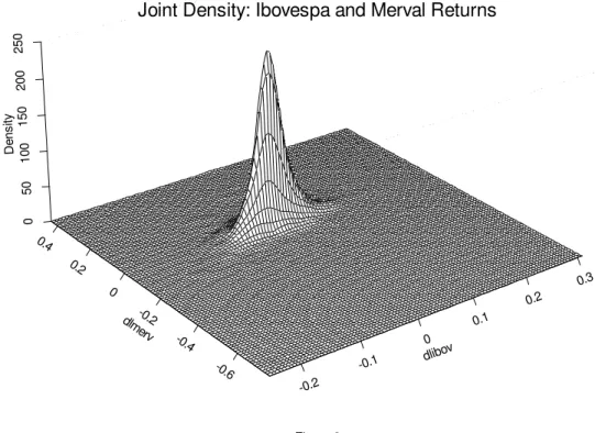
'HQVLW\HVWLPDWLRQ
The densities of both Ibovespa and Merval returns are characterised by heavy tails.
Consider first the joint Ibovespa and Merval returns density, in Figure 3, and then the
non-parametric marginal densities estimates of each return compared to the normal densities
with same mean and variance in Figures 4 and 5. As the density estimates are inputs to the
estimation procedure, it is taking into account the heavy tails which characterise the data at
stake.
,W{FRYDULDQFHHVWLPDWLRQWKHGRXEOH9DVLFHNDQG&,5PRGHOV
Given the estimates for θL, &L , i = 1,2, and the density estimates for π(.,.) and πL(.), i=1,2,
the covariance estimate σˆ12 solves (19) and (23), respectively, for the Vasicek and CIR
somewhat improperly, the &L estimates obtained above. This could be avoided by
considering more complex moment conditions which take into account the off-diagonal
terms of the Itô volatility matrix, as already mentioned in section 5.2.
---Insert Figures 3, 4 and 5 by here
---One important question concerning the boundary conditions remains. Consider first
the Vasicek model in the case of fixed income. At the point ([1,[2) = (0,0) one may rewrite
(20) as:
$1 = &2π(0,0)
$2 = π1(0)
2 1 3 =
$
0 1
1 1
1 ) (
=
[ G[
[ Gπ
∑
∑
= = =
−
= 2
1 0 2
1 2
4 (0, ) (0)
) ( 2
1
1 L
L L
[ L
L L
L L G[ [ G &
$ π µ θ π ,
if we impose π1(0) = π2(0) = π(0,0) = 0, which is the bivariate counterpart of Aït-Sahalia
(1996)’s boundary condition, the result is
2 / 1
0 2
1 2 1
0 1
1 1 12
) ( )
( )
0 (
1
− =
= =
−
=
∑
L [LL L
L L
[ G[
[ G & G[
[
Gπ π
It is straightforward to see that one may get a complex-valued boundary condition.
Imposing a real σ12(0) > 0 implies that
2 2 2 1 0 1 1 1 0 2 2 2 1 2 ) ( ) ( & & G[ [ G G[ [ G [
[ <−
= =
π π
,
as both & and & are assumed to be strictly positive and the derivatives are likely to have
the same (positive) sign, the assumption is invalid.
Consider next the Vasicek model in the case of variable income. Making π1([1min) =
π2([2min) = π([1min,[2min) = 0, one gets, at ([1,[2) = ([1min,[2min), for (20):
$1 = 0
$2 = 0
min 1 1 1 1 3 ) ( 2 1 [ G[ [ G
$ = π
∑
∑
= = − = 2 1 min min 2 1 24 ( , ) ( )
) ( 2 1 min L L L L L [ L L L L L [ [ G[ [ G & $ L π θ µ π leading to: 2 / 1 min 1 2 1 2 1 1 min 1 1 min 1 12 ) ( ) ( ) ( − =
∑
= − L L LL L G[
[ G & G[ [ G
[ π π
σ . (28)
Once again one may get a complex-valued boundary condition, what in fact
considered; given the results above, several were tried, and those actually used were
obtained as follows.
For the Vasicek model, assume that [1min is such that $1=0 and $4=0, a reasonable
assumption for our data set. The differential equation (19), related to the Vasicek model,
may then be written, at [1min , as
0 )
( ) (
3 min 1 1 12 1
min 1 12
2 + =
− [ $
G[ [ G
$ σ σ (29)
and, by straightforward calculation, one gets:
2 min 1 2 3 min
1 12( ))
log( [ .
$ $
[ =− +
σ ;
so that, assuming that .2 = 0:
−
= min
1 2 3 min
1
12( ) exp [
$ $ [
σ . (30)
Alternatively, one may set σ12([1min) = σ12’([1min) = Z and $1 = 0. This allows to
rewrite (19), at [1min , as:
($2 + $3) Z2 + $4 = 0 . (31)
The solutions are given by:
2 / 1
3 2
4 min
1
12( )
+ − ± = =
$ $
$ Z
[
σ . (32)
The solution of (19) subject to the boundary conditions (30) and (32) is rather
computer intensive. The negative root in (32) did not produce a sensible surface and, in all
cases, the numerical iterations did not converge for values of [1 (Ibovespa resturns) less
than –0.05. Moreover, for similar reasons, the range of [2 (Merval resturns) was restricted
Although each boundary condition may originate a completely different behaviour
for the covariance estimate, the shape in each of the two cases considered does not vary too
much along the range of [2, the returns of the Merval index. In fact, the two solutions
shown are flat for a considerably large range of [2 (say between –0.10 and 0.10). This may
indicate that there is independence between the covariance estimates and the variable [2, a
question that deserves more study in the future.
&21&/86,216
We developed an exploratory procedure to estimate and test two-dimensional diffusions
used in finance. The extension of Aït-Sahalia’s univariate idea to the bivariate case is not
immediate, since the solution of the corresponding Fokker-Planck equation can easily
become very difficult, if not impossible in analytical terms. By parametrizing the drifts of
both processes and imposing restrictions on the terms of the Itô and Fokker-Planck
covariance matrices, it is sometimes possible to obtain a nonparametric estimate of the
covariance between the processes. However, a delicate issue might still remain, regarding
the definition of the boundary conditions for the partial differential equations to be actually
solved.
Our main message is that extending in a general way Aït-Sahalia (1996)’s
framework to a multivariate setting is by no means straightforward. The basic reason is
perhaps because the correspondence between the Itô and Fokker-Planck representations in
higher dimensions is not the same as in the univariate case. For the methods developed
here, the Fokker-Planck is more tractable than the Itô representation, suggesting that
sensible assumptions on the drift and volatility functions, one cannot obtain a direct
generalisation of the univariate method.
Questions for improvement and further research include (i) the development of the
testing procedure concerning the differential equations resulting from the parametrizations
on the Itô volatilities in 3.2; (ii) the implementation of the estimation and testing procedure
sketched in section 3.3 and Appendix 1; (iii) the improvement of the GMM estimation
procedure used in section 5.2; (iv) alternative boundary conditions for differential equations
(19) and (22), as exemplified in 5.4; (v) the allowance of different bandwidths, taking also
into account the heavy tails of returns distributions, and the use of bivariate kernels which
would exploit better the dependence structure of the bivariate data. Moreover, by imposing
suitable regularity conditions on (a) the time series dependence in the data, (b) the kernels
actually used and (c) the bandwidths, asymptotic results must be developed for the various
estimators proposed.
Finally, a particular case that seems promising is that of “causal bivariate models” in
which one of the diffusions contributes to the volatility of the other. The appeal of this idea
is immediate – investors could improve their hedging strategies when considering a flexible
estimator of the covariance between two (groups of) assets of a given portfolio, instead of
assuming independence among processes and estimating separately univariate diffusions.
$&.12:/('*(0(176
We thank Getúlio B. da Silveira, Paulo Klinger Monteiro and the participants in the 1999
Forecasting Financial Markets, London, U.K., and the XXI Meeting of the Sociedade
the authors (Cristian Huse) acknowledges financial support from &RQVHOKR 1DFLRQDO GH
3HVTXLVDV±&13T, Brazil.
$33(1',;(67,0$7,1*)392/$7,/,7,(6
A natural way to obtain an estimator of the constant in E11(.), either in (25) or (26), is to
consider the kernel estimator of the conditional density using its definition:
) ( ˆ ) , ( ˆ ) ' , | , ( ˆ \ \ [ I W \ W [ I π
≡ (A1)
with [ = ([,[) and \ = (\,\), so that the numerator of the right-hand side of (A1) is the
joint density of two observations at the time distance (t’ + ∆t) – t’ = ∆t, which is the interval
between observations, and the denominator is the corresponding marginal density. The
(product) kernel estimators of the joint and marginal densities are given by, respectively,
∑
= − − − − = Q L LL L L L K \ \ . K \ \ . K [ [ . K [ [ . QK \ [ I 1 2 2 1 1 2 2 1 1 4 1 ) , (ˆ (A2)
and − − =
∑
= K \ K \ \ . QK \ L Q LL 2 2
1 1 1 2 y K 1 ) ( ˆ
π (A3)
where the kernel .(.) is a symmetric, finite variance, univariate density, and the parameter
K, assumed to be the same for every kernel, is the bandwidth.
The marginal Iˆ1([1|\) of the bivariate conditional Iˆ([ | \) will be:
∫
∫
=≡ 2 2
1
1 ˆ( , )
) ( ˆ 1 ) ( ˆ ) , ( ˆ ) | (
ˆ I [ \ G[
\ G[ \ \ [ I \ [ I π
By defining X = ([ – [L)/K, integrating (A4) with respect to X, and using the fact that the
kernel function is a density, one obtains
∑
∑
= = − − − − − = Q L L L Q L L L L K \ K \ \ . K \ K \ \ . K [ [ . K \ [ I 1 2 2 1 1 1 2 2 1 1 1 1 1 1 y K y K 1 ) | (ˆ , (A5)
which can be used to compute the marginal variances for selected \M = (\M,\M).
By defining Y = ([ – [L)/K, integrating with respect to Y, and using the properties of
the kernel function, one obtains for the marginal mean:
∑
∑
= = − − − − = Q L L L Q L L L K \ \ . K \ \ . K \ \ . K \ \ . [ 1 2 2 1 1 1 2 2 1 1 1 1 ˆµ (A6)
and for the marginal variance
∑
∑
= = − − − − − = Q L L L Q L L L K \ K \ \ . K \ K \ \ . [ E 1 2 2 1 1 1 2 2 1 1 2 1 1 11 y K y K ) ˆ ( ˆ µ (A7)Fitting a line through the points \M = (\M,Eˆ11(\M)) plus the origin will produce an
estimate for N1.
A second idea – likely to be more demanding and dependent on approximations –
starts by recalling that, for small displacements τ = t – t’, if the derivatives of the FP drifts
and volatilities are negligible compared of those of the transition density, the equation to be
∑∑
∑
= = = ∂ ∂ ∂ + ∂ ∂ − = ∂ ∂ 2 1 2 1 2 2 1 ) ’ , | , ( ) ( 2 1 ) ’ , | , ( ) , ( ) ’ , | , (L M LM L M
L L L [ [
W \ W [ I \ E [ W \ W [ I \ W \ W [ I
W µ θ . (A8)
Subject to the initial condition
I([,W;\,W’)=δ([−\) ,
the solution to this equation will be a Gaussian distribution, with mean \ + µ(\W¶θ)(W±W¶) ,
whose covariance matrix coincides with that of the FP E’s (see Gardiner (1997), section
3.5):
⋅ −
= − /2 1/2 −1/2
) ’ ( )]} ’ , ( {det[ ) 2 ( ) ’ , | ,
([ W \ W % \ W W W
I π 1
− − − − − − − − ⋅ − ) ’ ( )] ’ )( ; ’ , ( [ )] ’ , ( [ )] ’ )( ; ’ , ( [ 2 1 exp 1 W W W W W \ \ [ W \ % W W W \ \
[ µ θ 7 µ θ
(A9) where = ) ’ , ( ) ’ , ( ) ’ , ( ) ’ , ( ) ’ , ( 22 12 12 11 W \ E W \ E W \ E W \ E W \ % , = 2 1 [ [ [ , = 2 1 \ \ \ , = ) ; ’ , ( ) ; ’ , ( ) ; ’ , ( 2 2 1 1 θ µ θ µ θ µ W \ W \ W \ .
Recalling that – under stationarity – the left hand side of (A9) is estimable using
(A1)-(A3), this opens a range of possibilities both for estimation and testing. With the
parametrizations at stake - in a “CIR or Vasicek fashion” - the parameter N1 is not known
but, if one estimates parameter N2 (e.g. by GMM) and takes (12) into account, inserting it
into (A9), E12(\) is eliminated and there is only one unknown in this equation – N1. One
between the associated bivariate normal density and the one estimated non-parametrically.
Again, once N1 is obtained, E12(\) follows in a straightforward manner.
Finally, if the assumptions leading to (A9) are considered reasonable, it is also
possible to test a variety of hypotheses comparing the densities I([,W|\,W’) resulting from
the two alternatives. For instance, one could compare different parametrizations concerning
both the drifts and volatilities of the bivariate process.
5()(5(1&(6
Aït-Sahalia, Y. (1996) Nonparametric Pricing of Interest Rate Derivative Securities,
(FRQRPHWULFD, , 527-560.
Black, F., and Scholes M. (1973) The Pricing of Options and Corporate Liabilities, -RXUQDO
RI3ROLWLFDO(FRQRP\, , 637-654.
Brennan, M. and Schwartz, E. (1979) A Continuous Time Approach to the Pricing of
Bonds, -RXUQDORI%DQNLQJDQG)LQDQFH, 133-155.
Cox, J., Ingersoll J.and Ross S. (1985a) An Intertemporal General Equilibrium Model of
Asset Prices, (FRQRPHWULFD, , 363-384.
Cox, J., Ingersoll J.and Ross S. (1985b) A Theory of the Term Structure of Interest Rates,
(FRQRPHWULFD, , 385-407.
Davidson, R., and MacKinnon J. G. (1993) (VWLPDWLRQDQG,QIHUHQFHLQ(FRQRPHWULFV,
Oxford: Oxford University Press.
Duffie, D., and Singleton K. (1993) Simulated Moments Estimation of Markov Models of
Asset Prices, (FRQRPHWULFD, , 929-952.
Gourieroux, C., Monfort A. and Renault E. (1993) Indirect Inference, -RXUQDORI
$SSOLHG(FRQRPHWULFV, , S85-S118.
Hull, J. and White A. (1987) The Pricing of Options on Assets with Stochastic Volatilities.
-RXUQDORI)LQDQFH, , 281-300.
Karlin, S., and Taylor H.M. (1981): $6HFRQG&RXUVHLQ6WRFKDVWLF3URFHVVHV, New York:
Academic Press.
Lo, A. W. (1988) Maximum Likelihood Estimation of Generalized Itô Processes with
Discretely Sampled Data, (FRQRPHWULF7KHRU\, , 231-247.
Merton, R.C. (1973) Theory of Rational Optional Pricing, %HOO-RXUQDORI(FRQRPLFVDQG
0DQDJHPHQW6FLHQFH, , 141-183.
Nelson, D.B. (1990) ARCH Models as Diffusion Approximations, -RXUQDORI
(FRQRPHWULFV, , 7-38.
Pritsker, M. (1998) Nonparametric Density Estimation and Tests of Continuous-Time
Interest Rate Models, 5HYLHZRI)LQDQFLDO6WXGLHV: 449-487.
Scott, D.W. (1992) 0XOWLYDULDWH'HQVLW\(VWLPDWLRQ7KHRRU\3UDFWLFHDQG
9LVXDOL]DWLRQ, New York: Wiley.
Silverman, B.W. (1986) 'HQVLW\(VWLPDWLRQIRU6WDWLVWLFDODQG'DWD$QDO\VLV, London:
Chapman and Hall.
Vasicek, O. (1977) An Equilibrium Characterization of the Term Structure, -RXUQDORI
0 500 1000 1500 2000
-0
.2
-0
.1
0
.0
0
.1
0
.2
0
.3
Ibovespa Returns
Figure 1
0 500 1000 1500 2000
-0
.8
-0
.6
-0
.4
-0
.2
0
.0
0
.2
0
.4
Merval Returns
-0.2
-0.1 0
0.1 0.2
0.3
dlibov
-0.6 -0.4 -0.2 0 0.2 0.4
dlm erv
0
5
0
1
0
0
1
5
0
2
0
0
2
5
0
D
e
n
s
it
y
Joint Density: Ibovespa and Merval Returns
Figure 3
-0.2 -0.1 0.0 0.1 0.2 0.3
0
1
0
0
0
2
0
0
0
3
0
0
0
Daily Returns
D
e
n
s
it
y
Nonparametric Density: Ibovespa x 'Normal' Ibovespa (in circles)
-0.8 -0.6 -0.4 -0.2 0.0 0.2 0.4
0
5
0
0
1
0
0
0
1
5
0
0
2
0
0
0
2
5
0
0
3
0
0
0
Daily Returns
D
e
n
s
it
y
Nonparametric Density: Merval x 'Normal' Merval (in circles)