Bio-inspired Artificial Intelligence:
А
Generalized Net
Model of the Regularization Process in MLP
Stanimir Surchev1, Sotir Sotirov1, Wojciech Korneta2
1
“Prof. Dr. Assen Zlatarov” University Burgas, Bulgaria
E-mails: [email protected], [email protected]
2
College of Computer Science and Business Administration in Łomża 14, Akademicka, 18-400 Łomża, Poland
E-mail: [email protected]
Received: July 3, 2013 Accepted: October 04, 2013
Published: October 15, 2013
Abstract: Many objects and processes inspired by the nature have been recreated by the scientists. The inspiration to create a Multilayer Neural Network came from human brain as member of the group. It possesses complicated structure and it is difficult to recreate, because of the existence of too many processes that require different solving methods. The aim of the following paper is to describe one of the methods that improve learning process of Artificial Neural Network. The proposed generalized net method presents Regularization process in Multilayer Neural Network. The purpose of verification is to protect the neural network from overfitting. The regularization is commonly used in neural network training process. Many methods of verification are present, the subject of interest is the one known as Regularization. It contains function in order to set weights and biases with smaller values to protect from overfitting.
Keywords: Neural network, Generalized net, Supervised learning, Overfitting, Regularization.
Introduction
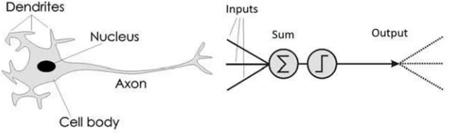
Neural Networks are an abstract representation, bio-inspired from human brain neural system [4]. All elements of the artificial neuron are taken from the biological neuron (Fig. 1).
An electrical signal has been received in a biological neuron from other neurons, and conveyed to the cell body by dendrites. Resultant electrical signals are sent along the axon in order to be distributed to other neurons. The artificial neuron operates by analogy. Activation signals from other neurons are summed in the neuron and passed through an activation function and the resulting value is further sent to the other neurons [8].
Fig. 1 Comparison between biological and artificial neuron
unsupervised and supervised [7]. The problem of overfitting is frequently met in the learning process [3]. It appears in different situations, affects the trained parameters and worsens the output results. There are different methods that can help avoiding the overfitting, namely Early Stopping and Regularization. In [6], we described the process of Early Stopping. The process of Regularization is described below.
The general idea of the Regularization method is to improve the performance function and this is the reason why the described neural network with generalized net exhibits the moment where the training process obtains the coefficients of weights and biases.
The first step is to prepare the necessary data of neural network. The data contains input and target matrix, which must have an equal number of vectors:
1,1 1,
,
,1 ,
j
i j
i i j
p p
p
p p
where i is the maximum number of vectors in input data; and j is the maximum number of elements of input vector; and
1,1 1,
,
,1 ,
n
m n
m m
t t
t
t t
n
where m is the maximum number of vectors in target data; and n is the maximum number of elements of target vector.
When the matrices are obtained, the next step is to choose the type of neural network and necessary parameters and after that the training process can begin. The program source code for creation of the neural network has the following requirements:
min i,1 max i,1 ; ; min i j, max i j, , ; , ' ' , ' ' , 'i 0 '
net p p p p G h F F Ft
,(1)
where net is the set of elements for creating the feedforward neural network;
,
min pi j , max pi j are the minimal and maximum elements value of column; G is the
number of hidden neurons; h is the number of outputs neurons; Fi is the performance function
of input data; F0 is the performance function of output data; Ft is the training function. It
updates values of weight and bias matrixes, where depending of training method. The following formulae can be changed:
1
ˆg g
g
F
w k w k
w
(2)
1
ˆg g
g
F
b k b k
b
where g is the current neuron; k is the current number of iteration; Fˆg
w
is the modification function.
When the input parameters are prepared, the next step is to calculate and train the neural network. The basic parameter that is necessary for training process is the performance function, and the algorithm of mean squares error (MSE) is basically used:
2
2(4)
1 1
1 N 1 N
i i i
i i
mse e t a
N N
where a is the output data;
1
N
i i i
a f p w b
(5)and t is the target data; N is the maximum number of training pairs (p, t); e is the error between output and target data.
The Regularization method changes the formula of MSE:
* 1 *
msereg mse msw (6)
where is the performance parameter with ג [0÷1]. Its value is very important, because the
line between good and overfit output data is very small.
2 1
1 n j j
msw w
n
(7)where msw – mean square weights; n – maximum number of weights.
The modification of the performance function reduces the weight and bias values. This influences the results, making them smoother and decreasing the chance of overfitting.
GN-model
Initially, the following tokens enter in the GN [1]:
In place L1 – α token with initial characteristic “Input and target vectors”
0
x“ pi j, , tm n, ”;
In place L5 – token with initial characteristic “Structure of neural network”
0
x “net”;
In place L6 – token with initial characteristic “Maximum number of iteration and
minimum value of performance function”
0
In place L7 – token with initial characteristic “Performance parameter”
0
x “ ”;
In place L19 – token with initial characteristic “Initial and maximum corrections”
0
x “Ks 0, Kmax”.
The GN presented on Fig. 2 by the following set of transitions: A = {Z1, Z2, Z3, Z4}. These
transitions describe the following processes:
Z1 = “Preparing of data”;
Z2 = “Training of neural network”;
Z3 = “Computing mean square error with regularization”;
Z4 = “Correction, if overfit”.
Z3 Z4
Z2 Z1
L8 L1
L2
L5
L3 L2
L1 L
9
L1 L6
L4
L2 L1
L7
L1 L1
L1
L2
L1 L1
Fig. 2
Z1 = {L1, L4, L20}, {L2, L3, L4}, R1, (L1, L4, L20),
2 3 4
1 1
4 4,2 4,3
20
,
L L L
R
L False False True
L W W True
L False False True
where W4,2 = “i = m”; W4,3= ¬W4,2.
The token α enters place L4 from place L1 and does not obtain any new characteristic. It stays
in place L4 during the whole functioning of the GN. The token α enters place L2 from place L4
L1
L1
and does not obtain any new characteristic. The token α enters place L3 from place L4 and
does not obtain any new characteristic.
Z2 = {L2, L5, L6, L7, L10, L11, L12, L13, L14, L22}, {L8, L9, L10, L11, L12, L13}, R2,
( (L2, L5, L7), L6, L10, L11, L12, L13, L14, L22)),
8 9 10 11 12 13
2 2 5 6 7
10 10,9 10,12
11 11,9 11,10
L L L L L L
R
L False False False False False True
L False False False False False True
L False False True True False False
L False False False False False False
L False W True False W False
L False W W True F
12 12,8
13 13,12
14 22
,
alse False
L W False False False True False
L False False False False W True
L False False False True False False
L False False True True False True
where
W10,9 = “Icu = Imax”; W10,12 = ¬W10,9;
W11,9 = “Fmsereg≤Mmin”; W11,10 = ¬W11,9;
W12,8 = “Computed weights and biases”;
W13,12 = “Necessary data for training are obtained”.
The tokens α, , from places L2, L5, L7 unite in one token in place L13 and this new token
obtains the new characteristic “Necessary data for training of neural network”. The token splits in two equal tokens, accordingly: the first one enters place L12 and obtains a new
characteristic “Weight and bias data”, while the second one stays in place L13 for the whole
functioning of the GN.
cu
x “x0, , , , x0 x W b0 ”
The token from place L6 splits in two tokens and , in places L10 and L11 accordingly,
and these obtain the respective new characteristics: “Maximum number of iterations” and “Minimum number of performance function”:
’
cu
x “Imax”;
’’
cu
x “Mmin”.
The token from place L12 splits in two tokens
and
, where the first token enters placeL8, and the second one enters place L12, and they accordingly obtain the following new
characteristics “Data for computing of performance function” and “Necessary data for training”:
’
cu
x “p t F W b x, , , , , t 0 ”;
’’
cu
The token from place L11 enters place L9, where it does not obtain any new characteristic.
The token from place L11 enters place L10, where it obtains the new characteristic “Current
number of iterations”:
cu
x “Fmsereg,Icu”;
Icu+1=Icu + 1.
The token from place L10 enters place L9, and does not obtain any new characteristic. The
token from place L10 enters place L12, and again does not obtain any new characteristic.
Z3 = {L8, L15, L16, L17, L18}, {L14, L15, L16, L17, L18}, R3, ( (L16, L17), L8, L15, L18),
14 15 16 17 18
3 8
15 15,14
16 16,15
17 17,15
18 18,17
,
L L L L L
R
L False False True False True
L W True False False False
L False W True False False
L False W False True False
L False False False W True
where
W15,14 = “Computed mean square error with regularization (msereg)”;
W16,15 = “Computed mean square weights (msw)”;
W17,15 = “Computed mean square error (mse)”;
W18,17 = “Computed output data (а)”.
The token ’ from place L8 splits in two tokens: 1' and 2' that enter places L16 and L18. They
obtain there the following new characteristics, accordingly; “Mean square weights” and “Output data”:
' 1
cu
x “x W b F0, , , msw”;
' 2
cu
x “t p W b F a, , , , , t ”.
The token 2 from place L18 splits in two tokens: the first token 21 enters place L17 and
obtain the new characteristic “Mean square error”, while the second token 22 stays in place
L18 for the whole functioning of the GN: ' 21
cu
x “t a F, , mse”;
' 22
cu
x “ , , , p W b Ft”.
The token 1 from place L16 splits in two tokens: the first token 11 enters place L15, and the
second token 12 remains looping in place L16 for the whole functioning of the GN: '
11
cu
x “x0, Fmsw”;
' 12
cu
x “W b, ”.
The token 21 from place L17 splits in two: the first token 211 enters place L15, while the
' 211
cu
x “Fmse”;
' 212
cu
x “t a, ”.
The tokens 11 and 211 from places L16 and L17 unite in one token in place L15 and that new
token obtains the characteristic “Mean square error with regularization”. The token splits in two: the first token enters place L14, while the second token remains to loop in place L15
for the whole functioning of the GN:
cu
x “Fmse, , x0 Fmsw”;
cu
x “Fmsereg”.
The token from place L15 enters place L14 where it does not obtain any new characteristic.
Z4 = {L9, L19, L23}, {L20, L21, L22, L23}, R4, (L9, L19, L23),
20 21 22 23
4 9 19
23 23,20 23,21 23,22
,
L L L L
R
L False False False True
L False False False True
L W W W True
where W23,21 = “Network is not overfit”; W23,20 = W23,22 = ¬W23.21.
The token from place L9 enters place L23 and obtains there a new characteristic “Current
number corrections”:
Kcu+1 = Kcu + 1.
The token obtains the following characteristics:
When transferring from place L23 to place L20, it obtains the new characteristic
“Correction of input and target data”;
When transferring from place L23 to place L21, it obtains the new characteristic
“Correct trained neural network”;
When transferring from place L23 to place L22, it obtains the new characteristic
“Correction of necessary training data”.
Conclusion
In the present paper, one of the methods of verification of neural networks, namely Regularization, has been described by the apparatus of generalized nets. The main function of this method is to decrease weight and bias values by modification of the performance function. This modification reduces the percentage of overfitting.
References
1. Atanassov K. (1991). Generalized nets, World Scientific, Singapore, New Jersey, London.
2. Hudson B. M., M. T. Hagan, H. B. Demuth (2012). Neural Network Toolbox User’s Guide R2012a 1992-2012.
3. Geman S., E. Bienenstock, R. Doursat (1992). Neural Networks and the Bias/Variance Dilemma, Neural Computation, 4, 1-58.
5. Morgan N., H. Bourlard (1990). Generalization and Parameter Estimation in Feedforward Nets, 630-637.
6. Tikhonov A. N. (1963). On Solving Incorrectly Posed Problems and Method of Regularization, Doklady Akademii Nauk USSR, 151, 501-504.
7. Widrow B., M. Hoff (1960). Adaptive Switching Circuits, IRE WESCON Convention Record, 96-104.
8. www.webpages.ttu.edu/dleverin/neural_network/neural_networks.html (access date July 3, 2013).
Stanimir Surchev, M.Sc. E-mail: [email protected]
Stanimir Surchev graduated from “Prof. Dr. Assen Zlatarov” University, Burgas, Department of Computers, Systems and Technologies in 2012. His research is in the field of chaotic signals using neural network. His current research interests are on neural network, chaos and computers.
Assoc. Prof. Sotir Sotirov, Ph.D. E-mail: [email protected]
Sotir Sotirov was graduated from Technical University in Sofia, Bulgaria, Department of Electronics. He received his Ph.D. degree from “Prof. Dr. Assen Zlatarov” University, Burgas in 2005. His current research interests are in the field of modeling of neural networks.
Wojciech Korneta, Ph.D., Dr. Hab. E-mail: [email protected]