Journal of Applied Fluid Mechanics, Vol. 10, No. 1, pp. 1-10, 2017.
Available online at www.jafmonline.net, ISSN 1735-3572, EISSN 1735-3645.
Dynamic Stall Prediction of a Pitching Airfoil using an
Adjusted Two-Equation URANS Turbulence Model
G. Bangga
1,2†and H. Sasongko
21 Institute of Aerodynamics and Gas Dynamics, University of Stuttgart, Germany 2 Mechanical Engineering Department, Institut Teknologi Sepuluh Nopember, Indonesia
†Corresponding Author Email: [email protected] (Received April 10, 2016; accepted August 24, 2016)
ABSTRACT
The necessity in the analysis of dynamic stall becomes increasingly important due to its impact on many streamlined structures such as helicopter and wind turbine rotor blades. The present paper provides Computational Fluid Dynamics (CFD) predictions of a pitching NACA 0012 airfoil at reduced frequency of 0.1 and at small Reynolds number value of 1.35e5. The simulations were carried out by adjusting the k −ε URANS turbulence model in order to damp the turbulence production in the near wall region. The damping factor was introduced as a function of wall distance in the buffer zone region. Parametric studies on the involving variables were conducted and the effect on the prediction capability was shown. The results were compared with available experimental data and CFD simulations using some selected two-equation turbulence models. An improvement of the lift coefficient prediction was shown even though the results still roughly mimic the experimental data. The flow development under the dynamic stall onset was investigated with regards to the effect of the leading and trailing edge vortices. Furthermore, the characteristics of the flow at several chords length downstream the airfoil were evaluated.
Keywords: Computational fluid dynamics; Flow turbulence; Pitching airfoil; Vortex flow.
N
OMENCLATUREc chord length
Cb damping factor according to realizable k – ε
Cl model lift coefficient
f damping factor as a step function fb damping factor
Gk production term for k Gɛ production term for ε k turbulent kinetic energy l turbulent length scale
Rec Reynolds number based on the chord length
S mean rate-of-strain tensor Sk user defined source for k Sɛ user defined source for ε TI turbulent intensity ui,j,k x,y,z velocities
u′i,j,k fluctuating x,y,z velocities V free stream velocity
x,y,z cartesian coordinates y+ non-dimensional wall distance Yk dissipation term for k Yɛ dissipation term for ε α angle of attack α0 mean angle of attack
ij kronecker delta
∆ oscillation amplitude ɛ energy dissipation
laminar viscosity t eddy viscosity density
σk turbulent Prandtl number for k
σɛ turbulent Prandtl number for ε ∅ phase angle
ˆωk reduced frequency, ωkc/2V
ωk angular velocity
1.
I
NTRODUCTIONThe aerodynamic loads of helicopter and wind turbine rotors have a strong time dependency
of dynamic stall is characterized by the formation of an intense vortical structure near the leading edge of the sectional airfoil causing the lift coefficient (Cl )
to increase beyond the static stall angle widely known as stall delay. This vortical structure is convected on the suction side of the airfoil indicated by the lift gradient increase. At a certain value of α near Cl,max, the vortex detaches from the airfoil body and starts to breaking down followed by the formation of the trailing edge vortex. This behavior is marked by a significant drop in Cl . The aerodynamic loads received by the structures usually is far greater thanin the static condition, increasing the stress field of the blade support system and has a huge potential to harm the structure itself (Witteveen et al. 2007).
Understanding the dynamic stall behaviour is important for accurate prediction of the aerodynamic loading on rotating machineries (Johansen 1999). Many studies have been conducted to reveal the dynamic stall mechanism (Bangga and Sasongko 2012; Naderi et al. 2016). Until the middle of 20th century, the dynamic stall was only studied experimentally due to limitation of the background data to govern the mathematical formulations. In the late of 1970s, Friedmann (Friedmann 1983) described three models and, afterwards, mathematical modelling on dynamic stall was developing (Hansen et al. 2004). The models ranged from fromsimple to complex such as ONERA (Petot 1989), Boeing (Friedmann 1983), Johnson (Johnson and Ham 1972; McCroskey et al. 1976), Øye (Øye 1991), Risø (Hansen et al. 2004) and also Leishman-Beddoes models (Leishman and Beddoes 1989; Hansen et al. 2004).
With the advent of computer performance, Computational Fluid Dynamics (CFD) simulations of the dynamic stall became possible. At the beginning, the compressibility effect was neglected due to limitation of the computational time (Fung and Carr 1991). This problem was brought up again to the surface in the late of ’90s by considering the compressibility and turbulence model influences (Ekaterinaris 1995; Ekaterinaris et al. 1995; Barakos and Drikakis 2003). However, due to the lack of robust CFD methods, most CFD works were done only focusing on the validation of the CFD codes rather than the physical phenomena of the flow. Wang et al. (Wang et al. 2010; Wang et al. 2012) demonstrated that the Shear-Stress-Transport (SST) k − ω turbulence model gave better prediction compared to the Wilcox k − ω for 2D case, but the predicted aerodynamic polar was rather non-smooth with a strong non-physical fluctuation along the whole range of α. Belkheir et al. (Belkheir et al. 2012) performed 2D and 3D CFD calculations of an airfoil using k −ε and SST k − ω models. The SST model gave a better pre-diction but the lift was overestimated and a strong fluctuation of the lift was observed in the down-stroke phase. Szydlowski and Costes (Szydlowski and Costes 2004) showed the prediction of static and oscillating airfoils using Unsteady Reynolds-Averaged Navier-Stokes (URANS), Detached Eddy Simulations (DES) and Large Eddy Simulations
(LES) models. The LES model clearly showed the superiority while the URANS and DES were struggling in predicting the laminar to turbulent transition, but the computational cost increased consider-ably in LES simulations.
Past studies on turbulent flow have shown that the accuracy of numerical predictions is signicantly affected by the accuracy of the employed turbulence model (Barakos and Drikakis 2003). The zero-equation turbulence model was shown to inaccurately predict separated flow by Baldwin and Lo-max (Baldwin and Lomax 1978). The linear eddy-viscosity models have several advantages in the prediction for turbulent flows. They provide satisfactory results for attached, fully developed turbulent boundary layers with weak pressure gradients and are also relatively easy to implement into CFD codes (Barakos and Drikakis 2003). Among them, two-equation eddy viscosity turbulence models were the most commonly used in practice.
It has been agreed that it was too naive and dangerous to assume the validity of a turbulence model in the wide range of flows (Arabshahi et al. 1998). It has been commonly known that the URANS models were inaccurate to predict the flow past airfoils beyond stall and often over predicted the maximum lift coefficient (Shur et al. 1999; Szydlowski and Costes 2004). Chitsomboon and Thamthae (Chitsomboon and Thamthae 2011) has shown that the overestimation came from the excessive turbulence level within the boundary layer, enhancing the momentum transfers to the near wall regions which helps the boundary layer to push through the ad-verse pressure gradient regions. The objective of the present study is to improve the prediction of the dynamic stall through an adjusted two-equation URANS turbulence model. The turbulence production is damped through the introduction of a damping function in the buffer zone. The k − ε turbulence model was chosen as the base be-cause it is one of the most commonly used turbulence models in industry and its simplicity makes the implementation of the damping factor easier. Parametric studies are conducted to observe the impact of the individual parameter implemented in the model. The study of the dynamic stall mechanism is conducted through an observation of the dynamic stall vortices. Finally, the wake flow pattern under dynamic motion of the airfoil is evaluated.
The paper is organized as follows. The test case and numerical procedures are given in section 2. Section 3 presents the results, and the conclusion is made in section 4.
2. C
OMPUTATIONALA
PPROACHES2.1 Adjustment of the Turbulence Model
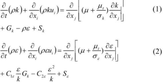
dynamics regarding the simulation of the mean flow characteristics for turbulent flow conditions. The model is governed by two transport equations, one for turbulent kinetic energy and one for its dissipation rate. The original model was proposed by Launder and Spalding (Launder and Spalding 1972) and has become the workhorse of practical engineering flow calculations in the time since then. The original k − ε or “standard” k − ε turbulence model is a semi-empirical model combined the exact equation for k and non-exact formulation for ε. The equation for dissipation rate was governed using physical reasoning and bears little resemblance to its mathematically exact counterpart. The transport equations for k and ε are given in Eqs. (1) and (2), respectively.
k k j k t j i i S G x k x ku x k t ( ) (1)
S k C G k C x x u x t k j t j i i 2 2 1 )( (2)
In these equations, Gk represents the generation of turbulence kinetic energy due to the mean velocity gradients, approximated in a consistent manner using oussinesq assumption, Gk = µt S2. S is defined as 2 . The turbulent viscosity is defined as
2k
C
f
b t
(3)
with Cµ is a constant with the value of 0.99. The other constants value are C1ε = 1.44, C2ε = 1.92, σε = 1.0, σε = 1.3.
Fig. 1. Damping as a step function for the case of
f = 0.1.
The only difference of the present modification with the original k −ε model is the addition of variable fb in Eq. (3). This parameter is defined as
.
b b
fC
f
(4) The parameter f is adopted from the near wall treatment according to Chitsomboon and Thamthae (Chitsomboon and Thamthae 2011) using step function, Fig. 1. The value of f is damped on the buffer zone around 5 < y+ < 30 and is unity on the other zones.Based on the knowledge on several turbulence models, realizable k −ε model (Shih et al. 1995) is likely perform better than the standard k − ε model in many aspects such as flows involving rotation, boundary layers under strong adverse pressure gradients, separation, and recirculation. Hence, we made use of this advantages and applied the damping factor, Cb, according to this model. It is defined as
* 1 0 1000 kU A A Cb (5)
With ij ij ij ij
S
S
U
*
~
~
(6)k ijk ij
ij
S
2
w
~
(7). 2 1 j i i j ij x u x u
S (8)
The constants A0 and A1 have the values of 4.04 and √6, respectively.
2.2 Test Case and Computational Mesh
This section provides the description of the numerical schemes used of the studied case. The commercial software package ANSYS Fluent 13.0 was used in this computation. Two dimensional analysis was selected because it is quite useful for observation of the flow characteristics and it can be useful in predicting the aerodynamic dependency of various parameters (Naderi et al. 2016). The SIMPLE algorithm was applied in the pressure velocity coupling and all equations to obtain a simultaneous solution (Wang et al. 2010). First order discretization for the momentum equations was used. It should be noted that the primary goal of this study is not to mimic the experiment results, but to demonstrate the improvement of the CFD predictions using the present modification. For the purpose of accurate simulations, the use of higher order schemes or even WENO scheme (Shu 2003) is strongly recommended. In this study, apart from the adjusted model, four other well-known turbulence models were used for comparison, namely standard k − ε, realizable k − ε, Wilcox k −ω and SST k −ω. The standard wall function was used for all k − ε based turbulence models.
airfoil was operating at the chord based Reynolds number of 1.35e5 with the chord length of c = 0.15m. The velocity, turbulent intensity and turbulent length scale at the inlet boundary was set equal to 14m/s, 0.08% and 0.0001m, respectively. The turbulent length scale near the airfoil can be approximated as l ~ cRe−1/5. The timestep was then calculated as ∆t = 2πl/V so that the timestep value is small enough to resolve the small eddies close to the airfoil.
Fig. 2. The mesh used in the calculations.
Fig. 3. Grid independency study. Airfoil grid points: Grid 1, 80 points; Grid 2, 120 points;
Grid 3, 204 points; Grid 4, 215 points.
The mesh was built using unstructured triangular mesh to accommodate the movement of the airfoil. It was modelled using the dynamic mesh approach with rigid body motion. Spring based smoothing scheme was adopted with the constant equal to zero, indicating zero damping value on the airfoil surface. The remeshing method was set on the local cells with the minimum length scale of 0m, maximum length scale of 0.8m, minimum cell skewness of 0.4
and size remeshing interval of unity. The number of grid points on the suction and pressure sides of the airfoil was 204. The mesh can be seen in Fig. 2. The inlet and the outlet boundaries were set as velocity inlet and pressure outlet boundary conditions, respectively, while the side wall boundary and the airfoil surface were non-slip walls. The grid studies were conducted using the standard k − ε turbulence model and the results are plotted in Fig. 3. Grid 3 was chosen and used for all simulations presented in this paper.
3. R
ESULTSA
NDD
ISCUSSION3.1 Parametric Study
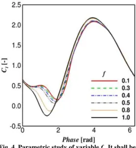
In this section, parametric study on the damping effects are given. The modification involves two main parameters, f and Cb, which give an impact on the prediction of the flow under dynamic stall for low Reynolds number. Fig. 4 shows the effect of the damping parameter f on the lift coefficient value at different phase angles. In these results, Cb was switched off (Cb = 1.0) for the isolation purpose. It can be seen that that the parameter has a strong impact on the predicted lift from the phase angles (φ) 0 to 5 radians. With decreasing damping value, f , the lift coefficient increases significantly at 0 < φ < 2 and reduces at 2 < φ < 5.
Fig. 4. Parametric study of variable f . It shall be noted that f = 1.0 represents no damping
condition.
Fig. 5. Relation between phase angle and α.
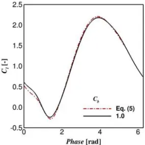
The introduction of parameter Cb gives a counter-balance of the results for the parameter f . Fig. 6 shows the effect of the parameter Cb on the lift pre-diction of an oscillating airfoil. It can be seen that the lift coefficient decreases at 0 < φ < 2. The cause of this reduction is the inclusion of rotation parameter in the governing equation in Section 2.1. Thus, the excessive momentum transfer of the flow over the suction side is alleviated, resulting in a smaller Cl value. On the other hand, Cl slightly increases at 2 < φ < 5, but in a smaller order of magnitude than Cl reduction for parameter f . Hence, the effect should be small.
Fig. 6. Parametric study of variable Cb. It shall
be noted that Cb = 1.0 represents no damping
condition.
3.2 Performance of the Modified Model
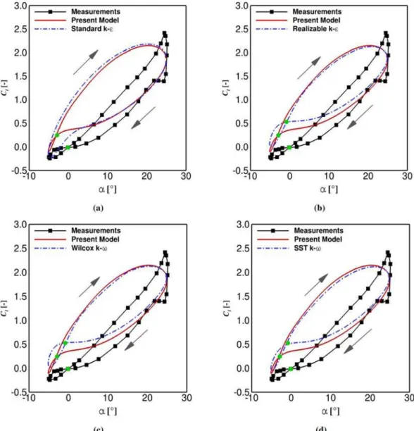
This section provides the comparison of the proposed model to some selected two-equation URANS turbulence models and measurement data from Lee and Gerontakos (Lee and Gerontakos 2004). Based on the parametric study in Section 3.1,
the damping factor is constructed by combining parameters f and Cb. The value of f = 0.3 was chosen in this work. The chosen value is based on the observation of the parametric study in Fig. 4. There can be seen that the resulting Cl distributions are similar for f = 0.1 − 0.5. Thus, it is recommended to choose the parameter value within this range.
Figure 7a shows the comparison of the present model to the standard k − ε turbulence model. It can be seen that the introduction of the damping parameter improves the prediction of the lift polar. The overestimated Cl for the whole upstroke phase is reduced although the reduction is not that significant. However, there is an important characteristic of the oscillating airfoil which cannot be predicted using the standard model: the switch of the lift behaviour at small angles of attack which produces the bundle of Cl , the green circle dot in Fig. 7a. On the other hand, this behaviour can be predicted by the present model even though the location is not accurately estimated; αCFD = −2.8◦ and αExp. = 0◦.
The prediction using the realizable k − ε model in Fig. 7b shows a similar result with the present model. This characteristic comes from the fact that Cb in the present model was governed by mimicking the turbulence viscosity equation in the realizable k − ε model (Shih et al. 1995). However, the addition of parameter f improves the prediction of the lift. There is a massive reduction of Cl in the downstroke phase which makes the results closer to the measurement data. Both models successfully predicted the bundle of lift, but at different angle and at different value.
Flows over a low Reynolds number value are the speciality of the k − ω based turbulence models (Wilcox et al. 1998). The models predict in a good agreement for many engineering applications involving shear flows (Hutomo et al. 2016; Bangga et al. 2015b; Bangga et al. 2015a). The predictions using these models are presented in Figs. 7c and 7d. Similar with the realizable k − ε model, the proposed model predicts very similar results with the Wilcox k −ω and SST k −ω turbulence models. The improvements are observed in the downstroke phase and all models can predict the lift bundle. It should be noted that the prediction of the bundle using the modified k −ε model is very similar with the SST model (Fig. 7d). The value is better predicted using the present model but the location is otherwise.
Fig. 7. Comparison of the present model to the other two-equation URANS models.
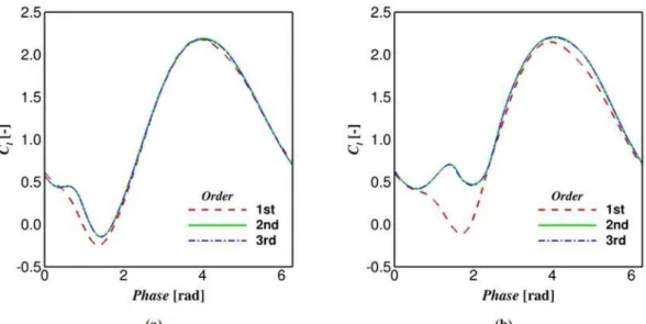
The other reasons are related to the numerical schemes and discretization. As mentioned in Section 2.2, the goal of the present work is not to accurately predict the forces but to demonstrate the improvement of the modification using a small order discreatization for faster and simpler analyses. The effect of numerical discretization is presented in Fig. 8. It can be seen that discretization order shows strong impact on both turbulence models, standard and adjusted k − ε. The impact is more pronounced around 0 < φ < 2.5 and 4 < φ < 6. Converged results with regard to the discretization order is shown for the 2nd order case. Therefore, it is recommended to use 2nd order discretization for future simulations.
3.3 Dynamic Stall Mechanism
To better understand the dynamic stall characteristics, this section provides the analyses of the vortical structures development under dynamic stall and their impact on the near wake region. Fig.
9 shows the plot of vorticity in the spanwise direction for different angles of attack during the full cycle of dynamic stall onset at low Reynolds number.
Fig. 8. Discretization order impact for (a) standard and (b) adjusted k −ε models.
Just right after the downstroke phase begins, the boundary layer thickness near the leading edge on the suction side grows rapidly, creating separation and reattachment mechanism which produces the leading edge vortex. This vortex travels down-stream with decreasing α value, shown in Figs. 8h -8l, which preserves even until the end of the down-stroke phase. In consequence, the lift increases at small angle of attack in the downstroke phase. On the other hand, the breakdown of the leading edge vortex, observed in the upstroke phase at small α (Fig. 9a), contributes to the reduction of lift. This creates the bundle of lift polar observed in Fig. 7.
This characteristic is different with the general dynamic stall behaviour in which the shedding of the leading edge vortex occurs in the up-stroke phase. McCroskey et al. (McCroskey et al. 1976) explained this behaviour as the phase shift and it is strongly influenced by the reduced frequency. Bangga and Sasongko (Bangga and Sasongko 2012) performed CFD simulations of an oscillating rotocraft airfoil at a reduced frequency of 0.62. They observed an alternating domination of the leading edge and the trailing edge vortices at high angles of attack, resulting in the lift fluctuation. It is strongly different with the present study ( ˆωk = 0.1) which shows the domination of the fully attached flow for the upstroke phase, even at high angles of attack.
The phase shifting explained above is strongly influenced by the adverse pressure gradient and the location of the stagnation point which moves periodically with the change of the angle of attack. The stagnation location is shifted far downstream at high angle of attack, and this produces a very strong positive pressure gradient. In consequence, flow separation occurs on the leading edge. However, since the airfoil is fastly pitching, there is an additional circulation induced by the uptroke motion which makes the flow remains attached.
For instance see Fig. 8f where the flow is fully attached.
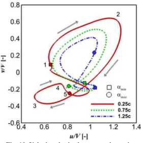
In addition to the phase shifting explained above, three observation points downstream of the airfoil were monitored during the simulations for the analysis of the near wake region. They are located at 0.25c, 0.75c and 1.25c behind the airfoil. The extracted data are the instantaneous velocities in the x− and y−directions and the results are plotted in Fig. 10.
It can be seen that the velocity range during the cycle of the dynamic stall onset decreases with in-creasing chordwise distance from the trailing edge. For instance, the ranges for the observation point of x/c = 0.25 are 0.5 < u/V < 1.23 and −0.34 < v/V < 0.6. They are reduced by 37% (x/c = 0.75) to 56% (x/c = 1.25) for x−velocity and 24% (x/c = 0.75) to 35% (x/c = 1.25) for y−velocity.
What interesting is that the upstroke motion occupies a longer velocity plot line than the down-stroke motion, and the difference decreases with the downstream distance. It can be divided into four main categories, see Fig. 10. Zone (1)-(2) is where the leading edge vortex detaches from the airfoil body and interacts with the trailing edge vortex so that y−velocity increases (Fig. 9a). Zone (2)-(3) shows the typical velocity characteristic for a fully attached flow; x− and y−velocities decrease with α. Zone (3)-(4) is where the boundary layer thick-ness thickening starts and Zone (4)-(5) is where the leading edge vortex is formed.
Fig. 9. Development of the leading edge vortex colored by spanwise vorticity value in [1/s].
4. C
ONCLUSIONIn the present study, an oscillating airfoil has been simulated using an adjusted two-equation turbulence model. A damping factor was introduced and implemented in the standard k − ε turbulence model. The proposed damping was governed based on the wall distance and a parameter which was
Fig. 10. Velocity plot in the near wake region.
The dynamic stall phenomenon studied in this work was observed through the observation of the vortex development. The leading and trailing edge vortices were captured in the present study. The phase shifting occurred and the convection of the leading edge vortex was observed in the downstroke phase. This phenomenon shows a strong impact on the near wake flow behind the airfoil. The velocity ranges of a point downstream the airfoil de-crease with the distance from the specific point to the trailing edge, and this is highly influenced by the reduced frequency.
The present study accompanied only a specific case and it was calculated with the low order numerical schemes for faster and simpler analyses. It has been shown that numerical scheme order affected the force prediction. For future studies, it is suggested to use at least 2nd order schemes for accurate results. Furthermore, because the onset of dynamic stall is actually 3D effects, 3D CFD simulations are encouraged to be performed.
A
CKNOWLEDGMENTThe authors would like to acknowledge the Ministry of Research, Technology and Higher Education of Indonesia for the financial support through DGHE scholarship.
R
EFERENCESArabshahi, A., M. Beddhu, W. Briley, J. Chen, A. Gaither, J. Janus, M. Jiang, D. Marcum, J. McGinley, R. Pankajakshan and et al. (1998). A perspective on naval hydrodynamic flow simulations. In Proceeding of 22nd ONR Symposium on Naval Hydro 920–934.
Baldwin, B. S. and H. Lomax (1978). Thin layer approximation and algebraic model for separated turbulent flows. American Institute of Aeronautics and Astronautics 257.
Bangga, G. and H. Sasongko (2012). Numerical investigation of dynamic stall for
non-stationary two-dimensional blade airfoils. In Annual Thermofluid Conference 4, 106–112. Bangga, G. S. T. A., T. Lutz and E. Krämer
(2015b). Numerical investigation of unsteady aerodynamic effects on thick flatback airfoils. In Proceeding of German Wind Energy Conference 12, Bremen, Germany 76.
Bangga, G., T. Lutz, and E. Kr¨amer (2015a).An examination of rotational effects on large wind turbine blades. In 11th EAWE PhD Seminar, Stuttgart, Germany.
Barakos, G. and D. Drikakis (2003). Computational study of unsteady turbulent flows around oscillating and ramping aerofoils. International journal for numerical methods in fluids 42(2), 163–186.
Belkheir, N., R. Dizene and S. Khelladi (2012). A numerical simulation of turbulence flow around a blade profile of HAWT rotor in moving pulse. Journal of Applied Fluid Mechanics 5(1), 1–9.
Chen, S. H. and C. M. Ho (1987). Near wake of an unsteady symmetric airfoil. Journal of fluids and structures 1(2), 151–164.
Chitsomboon, T. and C. Thamthae (2011). Adjustment of k-ω SST turbulence model for an improved prediction of stalls on wind turbine blades. In Proceedings of the World Renewable Energy Congress 15, 4114–4120. Ekaterinaris, J. A. (1995). Numerical investigation
of dynamic stall of an oscillating wing. AIAA journal 33(10), 1803–1808.
Ekaterinaris, J., G. Srinivasan and W. Mc-Croskey (1995). Present capabilities of predicting two-dimensional dynamic stall. In AGARD Conference Proceedings, pp. 2–2. AGARD. Friedmann, P. (1983). Formulation and solution of
rotary-wing aeroelastic stability and response problems. Vertica 7, 101–141.
Fung, K. Y. and L. Carr (1991). Effects of com-pressibility on dynamic stall. AIAA journal 29(2), 306–308.
Hansen, M. H., M. Gaunaa and H. Madsen (2004). A Beddoes-Leishman type dynamic stall model in state-space and indicial formulations. Risø National Laboratory.
Hutomo, G., G. Bangga and H. Sasongko (2016). CFD studies of the dynamic stall characteristics on a rotating airfoil. Applied Mechanics and Materials 836, 109–114. Johansen, J. (1999). Unsteady airfoil flows with
application to aeroelastic stability. Risø National Laboratory.
Johnson, W. and N. D. Ham (1972). On the mechanism of dynamic stall. Journal of the American Helicopter Society 17(4), 36–45. Launder, B. E. and D. B. Spalding (1972). Lectures
Academic press.
Lee, T. and P. Gerontakos (2004). Investigation of flow over an oscillating airfoil. Journal of Fluid Mechanics 512, 313–341.
Leishman, J. G. and T. Beddoes (1989). A semi-empirical model for dynamic stall. Journal of the American Helicopter society 34(3), 3–17. McCroskey, W., L. Carr and K. McAlister (1976).
Dynamic stall experiments on oscillating airfoils. Aiaa Journal 14(1), 57–63.
Naderi, A., M. Mojtahedpoor and A. Beiki (2016). Numerical investigation of non-stationary parameters on effective phenomena of a pitching airfoil at low Reynolds number. Journal of Applied Fluid Mechanics 9(2), 643–651.
Øye, S. (1991). Dynamic stall simulated as time lag of separation. In Proceedings of the 4th IEA Symposium on the aerodynamics of wind turbines.
Petot, D. (1989). Differential equation modeling of dynamic stall. La Recherche Aerospatiale (English Edition) 5, 59–72.
Shih, T. H., W. W. Liou, A. Shabbir, Z. Yang and J. Zhu (1995). A new k- eddy viscosity model for high Reynolds number turbulent flows. Computers and Fluids 24(3), 227–238. Shu, C. W. (2003). High order finite difference and
finite volume WENO schemes and discontinuous Galerkin methods for CFD. International Journal of Computational Fluid
Dynamics 17(2), 107–118.
Shur, M., P. Spalart, M. Strelets and A. Travin (1999). Detached-eddy simulation of an air-foil at high angle of attack. Engineering turbulence modelling and experiments 4, 669– 678.
Szydlowski, J. and M. Costes (2004). Simulation of flow around a static and oscillating in pitch naca 0015 airfoil using urans and des. In Proceeding of ASME 2004 Heat Transfer/Fluids Engineering Summer Conference, 891–908. American Society of Mechanical Engineers.
Wang, S., D. B. Ingham, L. Ma, M. Pourkasha-nian and Z. Tao (2010). Numerical investigations on dynamic stall of low Reynolds number flow around oscillating airfoils. Computers and Fluids 39(9), 1529–1541.
Wang, S., D. B. Ingham, L. Ma, M. Pourkashanian and Z. Tao (2012). Turbulence modeling of deep dynamic stall at relatively low Reynolds number. Journal of Fluids and Structures 33, 191–209.
Wilcox, D. C. et al. (1998). Turbulence modeling for CFD, Volume 2. DCW industries La Canada, CA.
![Fig. 9. Development of the leading edge vortex colored by spanwise vorticity value in [1/s]](https://thumb-eu.123doks.com/thumbv2/123dok_br/17021970.232506/8.892.131.723.116.958/fig-development-leading-vortex-colored-spanwise-vorticity-value.webp)