THE STUDY OF DYNAMIC STALL AND URANS CAPABILITIES ON MODELLING PITCHING AIRFOIL FLOWS

ALEXANDRE FELIPE MEDINA CORREA

THE STUDY OF DYNAMIC STALL AND URANS

CAPABILITIES ON MODELLING PITCHING AIRFOIL FLOWS

UNIVERSIDADE FEDERAL DE UBERLÂNDIA

FACULDADE DE ENGENHARIA MECÂNICA

ALEXANDRE FELIPE MEDINA CORREA

Orientador

Prof. Dr. Francisco José de Souza

THE STUDY OF DYNAMIC STALL AND URANS CAPABILITIES ON

MODELLING AIRFOIL PITCHING FLOWS

Projeto de Conclusão de Curso apresentado ao Curso de Graduação em Engenharia Aeronáutica da Universidade Federal de Uberlândia, como parte dos requisitos para a obtenção do título de BACHAREL em ENGENHARIA AERONÁUTICA.

UBERLANDIA - MG

THE STUDY OF DYNAMIC STALL AND URANS CAPABILITIES ON

MODELLING AIRFOIL PITCHING FLOWS

Projeto de conclusão de curso APROVADO pelo Colegiado do Curso de Graduação em Engenharia Aeronáutica da Faculdade de Engenharia Mecânica da Universidade Federal de Uberlândia.

BANCA EXAMINADORA

________________________________________ Prof. Dr. Francisco José de Souza

Universidade Federal de Uberlândia

________________________________________ Prof. Dr. Odenir de Almeida

Universidade Federal de Uberlândia

________________________________________ Prof. MSc. Thiago Augusto Machado Guimarães

Universidade Federal de Uberlândia

UBERLANDIA - MG

ACKNOWLEDGEMENTS

I would like to firstly thank my parents, Yolanda and Eduardo, and to my family for the love and support, for being guidance when in trouble and comfort during the times of need. Especially to my sister, Ruth, for the friendship and for make me laugh as much as impossible every time back home.

A very special thanks to Dr. Steve Cochard, for his guidance and encouragement during my first experience with Computational Fluid Dynamics at The University of Sydney. Under his tutelage I developed focus and became interested in CFD, providing me with direction and support, being not only a mentor, but a true friend.

Thanks also go to my friends Dr. Thomas Earl and MSc. Joachim Paetzold, who provided me with technical advice and patience to guide me on the sharpening of my skills as a research student and future engineer. Also, for the many coffees shared near the university after lunch and just before coming back for work at the Hawkings Computing Laboratory and the Eagle’s Nest.

I would also like to thanks my friends from the First, Second, Third and Fourth classes of the Aeronautical Engineering Course, colleagues from the Laboratory of Fluid Mechanics and the professors from the Faculty of Mechanical Engineering, specially to my friends Déborah de Oliveira, Marcelo Samora, Caio Lauar, Bruno Ribeiro and Fernando Muniz; as well to the professors and friends Prof. Dr. Daniel Dall’Onder, Prof. Dr. Odenir de Almeida, Prof. Dr. Thiago Guimarães, Prof. Dr. Aldemir Cavalini Jr., Prof. Dr. Leonardo Sanches, Prof. MSc. Giuliano Venson and Prof. Dr. Aristeu da Silveira Neto.

“

Flying is learning how to throw yourself at

the ground and miss.”

Medina, A. F. The Study of Dynamic Stall and URANS capabilities on modelling Airfoil Pitching Flows. 2015. 50p. Graduation Project, Federal University of Uberlandia, Uberlandia, Brazil.

ABSTRACT

This document describes the investigation of the behavior of the flow over a pitching NACA 0012 airfoil at Reynolds number Re=100,000 and Re=2,500,000 of the analysis of a two-dimensional k-ω SST (Shear Stress Transport) simulation. The behavior of the flow wake at the trailing edge is studied by the analysis of streamlines for each incidence angle and results are compared by the study of theoretical concepts and experimental data. The use of standard Unsteady Reynolds-Averaged Navier-Stokes (URANS) simulation has shown accuracy in predicting stall and reattachment incidence angles for upstroke and downstroke. The simulations were also capable of capturing flow information in agreement with experiments despite the over prediction of lift and drag coefficients, due to the two-dimensional simplification. The study has also compared the two-dimensional URANS k-ω SST turbulence model simulation data with previous results from three-dimensional simulation Wall Resolved Large Eddy Simulation (LES) and two-dimensional URANS k-ε Chien turbulence model analysis, showing that the qualitative behavior of the hysteresis loop is close for the computations, although there is a quantitative deviation in the results for upstroke and downstroke in the lift coefficient.

KEYWORDS: _{dynamics stall, pitching airfoil, URANS, k-}ω SST turbulence modeling, sliding

Medina, A. F. The Study of Dynamic Stall and URANS capabilities on modelling Airfoil Pitching Flows. 2015. 50p. Projeto de Conclusão de Curso, Universidade Federal de Uberlândia, Uberlândia, Brasil.

RESUMO

O presente trabalho descreve a investigação do comportamento do escoamento sobre um aerofólio NACA 0012 em movimento de arfagem dinâmica em números de Reynolds Re=100,000 e Re=2,500,000 através da análise da simulação numérica bidimensional fazendo uso do modelo de turbulência k-ω SST (Shear Stress Transport). O comportamento da esteira do escoamento na região do bordo de fuga do aerofólio é estudado através da análise das linhas de corrente para cada ângulo de incidência durante o movimento de arfagem. Os resultados são comparados com estudos experimentais através de conceitos teóricos.

O uso das médias de Reynolds das Equações de Navier-Stokes, ou método URANS, mostrou acurácia na predição do estol dinâmico e dos ângulos de re-aderência da camada limite para movimento ascendente e descendente do aerofólio. A simulações também foram capazes de obter informações do escoamento em concordância com os resultados experimentais apesar da sobre-predição dos coeficientes de arrasto e sustentação, devido a abordagem bidimensional.

O estudo realizado também comparou os resultados da simulação bidimensional URANS do modelo de turbulência k-ω SST com análises encontradas em literatura para análise tridimensional via Simulação de Grandes Escalas (Wall Resolved LES) e também a simulação bidimensional URANS fazendo uso do modelo k-ε Chien, obtendo concordância qualitativa nos resultados dos três modelos, apesar de um visível desvio entre si para a análise do coeficiente de sustentação durante fases ascendente e descendente do movimento de arfagem.

PALAVRAS CHAVE: _{estol dinâmico, arfagem dinâmica, URANS, modelo de turbulência k-}ω

List of Figures

Figure 2.1-1 Flow structure analysis for static NACA 0012 airfoil (Gerontakos, 2004) ... 16

Figure 2.1-2 Dynamic stall stages for a pitching motion NACA0012 airfoil, adapted from Carr (1988) - Analysis of normal force and pitching moment coefficients ... 17

Figure 2.3-1Vortex model for a pitching flat-plate ... 22

Figure 2.3-2Lift Coefficient curves from the Theodorsen’s function for a flat-plate in pure pitch motion. The hysteresis loop enlarges and moves down with the increase of the reduced frequency (left) and thins as the pitch axis moves far from the leading edge (right) ... 27

Figure 4.2-1 Time averaging for stationary turbulence ... 30

Figure 4.2-2 Time averaging for nonstationary turbulence ... 31

Figure 5.1-1 Schematics for the NACA 0012 airfoil pitch motion ... 38

Figure 5.2-1 C-Grid computational domain mesh (left); internal circular domain for sliding mesh (center) and mesh interface domain connection –‘hanging nodes’ (right) ... 39

Figure 5.2-2 Sliding Meshes Concept applied to the internal circular domain for pitch motion 40 Figure 5.3-1Analysis of the influence of the average pitch step 𝛿𝛼 on the hysteresis loop for lift coefficient at Reynolds 105 and 2.5x106. The average pitch step was refined from 𝛿𝛼=0.0500⁰ to 𝛿𝛼=0.003125⁰... 42

Figure 6.1-1 Hysteresis loops obtained with two-dimensional RANS k-ω SST analysis for lift and drag coefficients compared to experimental results from Berton et al. (2002); k-ε Chien turbulence model simulations from Martinat et al. (2008) and LES simulations from Kasibhotla & Tafti (2014) and the application of Theodorsen’s Function (1934) ... 43

Figure 6.1-2 Vorticity colored streamlines for the NACA0012 pitching airfoil at 105 Reynolds number for the k-ω SST turbulence model, upstroke (↑) and downstroke (↓) phases ... 44

Figure 6.1-3 Analysis of flow behavior for ELDV (Berton et al., 2002) and k-W SST Analysis for 10⁰ and 14⁰, upstroke (↑) and downstroke (↓) phases ... 46

Figure 6.2-1 Hysteresis loops obtained with two-dimensional RANS k-ω SST analysis for lift and drag coefficients compared to experimental results from McAlister et al. (1978) and k-ε Chien turbulence model simulations from Martinat et al. (2008) and the application of Theodorsen’s Function (1934) ... 47

Figure 6.2-2 Vorticity colored streamlines for the NACA0012 pitching airfoil at 2.5x106 Reynolds number for the k-ω SST turbulence model, upstroke phase (↑) ... 48

Figure 6.2-3 Vorticity colored streamlines for the NACA0012 pitching airfoil at 2.5x106 Reynolds number for the k-ω SST turbulence model, downstroke phase (↓) ... 49

List of Tables

List of Abbreviations and Acronyms

CFD Computational Fluid Dynamics DDES Delayed Detached Eddy Simulation ELDV Embedded Laser Doppler Velocimetry LES Large Eddy Simulation

MFLab Laboratory of Fluid Mechanics NSE Navier-Stokes Equations OES Organized Eddy Simulation PIV Particle Image Velocimetry LDA Laser Doppler Anemometer LDV Laser Doppler Velocimetry LSV Laser Sheet Visualization Method RANS Reynolds-Averaged Navier-Stokes RNG Renormalization Group Theory SST Shear Stress Transport

UDF User Defined Function

List of Symbols

𝛼 Airfoil angle-of-attack [rad]

A Pitching axis position relative to chord from leading edge [-] 𝑏 Half chord (as conventional in Aeroelasticity), 𝑏 = 𝑐/2 [m]

𝑐 Airfoil chord [m]

𝐶(𝑘) Theodorsen’s Function [-]

𝐶𝐷 Drag coefficient [-]

𝐶𝐿 Lift coefficient [-]

𝐶𝑀 Momentum coefficient [-]

𝐶𝑃 Pressure coefficient [-]

𝛿𝛼̅ Average pitch step [rad]

ξ Stream-wise coordinate [-]

𝑘 Pitch reduced frequency, 𝜔𝑐/2𝑈_∞ [-]

𝐿(𝑡) Lift Force [N]

𝑅𝑒 Reynolds Number [-]

𝑈∞ Free-stream flow velocity [m/s]

T Pitching Period [s]

Contents

1 Introduction ... 14

2 Background Theory ... 16

2.1 The Dynamic Stall ... 16

2.2 Leading Studies on Dynamic Stall and Pitching Airfoils ... 18

2.3 The Theodorsen’s Function ... 21

3 Goals ... 28

4 Mathematical Modeling ... 29

4.1 Governing Equations ... 29

4.2 The Unsteady Reynolds-averaged Navier-Stokes ... 29

4.3 The Closure Problem ... 34

4.4 Turbulence Modeling ... 35

5 Numerical Setup ... 38

5.1 Physical Modelling ... 38

5.2 Computational Mesh ... 39

5.3 Procedure ... 40

6 Results and Analysis ... 42

6.1 Pitching Analysis at Reynolds Number 105 ... 43

6.2 Pitching Analysis at Reynolds Number 2.5x106 ... 46

7 Conclusions ... 52

Bibliography ... 53

Appendix ... 55

APPENDIX A – MATLAB Routines for the Analysis on Pitching Airfoils ... 56

1

Introduction

The flow past airfoils has been studied for almost a century when considering the Thin Airfoil Theory (Munk, 1922) applied to steady airfoils. These studies are the edge of aeronautical research, which allows the ongoing optimization of aeronautical profiles in modern aircraft. Unsteady effects used to be ignored for simplicity during experimental research; hence the flow over conventional fixed airfoils is widely studied and fairly well understood. However, this approximation is not sufficient to model the turbulent flow in the trailing edge during flight. Unsteadiness is an inherent part of the flow during flight, where there are far more variables that can change and cannot be accounted for during wind tunnel steady studies made on airfoils, hence, however the static stall and aerodynamics coefficients prediction are made considering well-developed flow past the airfoil in a quasi-steady condition it is necessary to do an unsteady analysis in order to capture dynamic stall characteristics.

Most aeronautical devices can encounter unsteady flow behavior during flight, whether designed for that or not. The unsteadiness is easily observable in the flow of rotorcraft devices and wind turbines, but also it is present in fixed wings, which can vibrate at high frequencies during flight, leading to undesirable problems as the flutter phenomena. The unsteadiness is also a way to delay dynamic stall to control periodic vortex generation and improve the performance of rotorcrafts and wind turbines (McCroskey, 1982).

Unsteady effects are also evident in the most fascinating spectacle, the flight of birds, which are not yet fully understood due to the challenges in creating and simulating a device that can reproduce all the motion characteristics of bird’s flapping wings. Nowadays, the modelling of flapping wings, or flapping airfoils when considering a two dimensional approach, is the combination of a plunging (or heaving) and pitching (oscillatory) motion. Considering this kind of motion, it is possible to see beneficial effects of unsteadiness, which is substantially important to the propulsive efficiency of flapping motion.

vorticity into the wake. When the pitching airfoil reaches a high incidence angle, the vortex has a high energy profile, causing vortex shedding at the leading edge and reaching dynamic stall, causing large loss in the lift and increasing drag. As the incidence angle decreases downstroke, the flow reattaches, delayed as compared to static stall, as found in the experiments of McAlister

et al. (1978) and Berton et al. (2002).

These unsteady effects can also be related to aeroelastic effects, where mutual interaction between aerodynamics and elastic forces on lifting surfaces is investigated. The aeroelastic effects are observable since the first attempts of flight, being the cause of many unsuccessful flights in the beginning of the 20th Century. The first model to linearize a the aeroelastic effects was based on small disturbance theory, by Theodore Theodorsen (1934), where the model coupled unsteady aerodynamics effects modelled by using the two-dimensional Bernoulli equations in a typical section, resulting in the first aeroelastic investigations (Johansen, 1999). Theodorsen then formulated a solution for the dynamic pitching airfoil in order to understand the flutter phenomenon.

The static stall can be characterized with the formation of a leading edge vortex and a laminar separation bubble close to the leading edge region, where the vortex travels along the surface and starts to grow. The static stall finally occurs when the vortex separates from the airfoil as it reaches the region close to the trailing edge.

Differently, in the dynamic stall the airfoil flow separation occurs at a higher angle-of-attack, where it can be characterized as a sudden drop of lift during the dynamic pitching motion. The shear layer near the leading edge rolls up to form the leading-edge vortex providing additional suction over the upper surface of the airfoil as it moves in the trailing edge direction. This additional suction allows a delay in the separation of the boundary layer. However, the boundary layer becomes unstable as the airfoil reaches higher incidence angles, leading to the dynamic stall. Dynamic stall is not a well-understood phenomenon yet, even when considering its importance to the performance and operational limits of helicopters, flapping wings, and wind turbines (McCroskey, 1982).

2

Background Theory

This chapter will present the literature review on the study and analysis of pitching airfoil flows as well as the underlying theory on dynamic stall and unsteady aerodynamics. It is important to firstly understand the mechanism of dynamic stall and the stages that can characterize it. Also, the main studies on the area are presented as a short description of the most important insights found by the researchers.

2.1 The Dynamic Stall

The static stall of an airfoil is an aerodynamic phenomenon characterized by flow separation and the decrease of lift. For steady airfoils, the flow encounters its wall and attaches to it, forming a laminar boundary layer. In the transitioning from laminar to turbulent flow, a separation bubble is formed close to the airfoil leading edge, creating a reverse flow region. Afterwards the boundary layer is reattached into turbulent flow until it reaches the trailing edge turbulent separation point, and thus creates a separated turbulent shear layer and the detached turbulent separation region. As the incident angles of the airfoil increases, the trailing edge separation point progress upward in the upper surface until it reaches the transition bubble. At this point the flow does not reattach after the laminar separation, the bubble “bursts” and then a separated turbulent flow region is created, leading to the stall of the airfoil by losing lift. The flow behaves in a different way for unsteady airfoils, since the vertical wake is now time-dependent due to the unsteadiness and the aerodynamics coefficients can change accordingly.

The stall of a body under unsteady motion is quite complex when compared to static stall (McCroskey, 1982). Dynamic stall is a phenomenon that occurs on lifting surfaces when the angle of attack increases at a finite rate until stall is produced, differently from the static stall since the angular velocity leads to the pitching motion and allows the airfoil to reach higher incidence angles than the one observed on the static case. The dynamic stall of a pitching motion can be characterized as either a rapid increase into the stall region or a harmonic oscillatory motion that leads to periodic vortex generation and stall and unstalling of the airfoil (Malone, 1974). As the pitching airfoil surpasses its static stall angle the flow is still attached to its surface and in a higher incidence angle it is possible to observe the appearance of reversal flow on its surface close to the trailing edge. As it moves upstroke (↑), large eddies appear in the boundary layer and the reversal flow starts to spread over the upper surface and a large leading edge vortex will appear causing the surge of the lift slope (Fig. 2.1-2).

Figure 2.1-2 Dynamic stall stages for a pitching motion NACA0012 airfoil, adapted from Carr (1988) - Analysis of normal force and pitching moment coefficients

incidence due to the flow acceleration (high Reynolds) or can be slow, finishing later on the upstroke phase of the pitch cycle to follow.

2.2 Leading Studies on Dynamic Stall and Pitching Airfoils

Numerous studies were made regarding the unsteady aerodynamics since the beginning of the 1930’s, as the first theories regarding the linearization of an unsteady function started. Due to the advance of measurement systems, experimental analysis was made in the late 1970’s and the 2000’s to investigate the periodic vortex formation and compare the flow behavior with respect to static results. Also, during the end of the 20th and beginning of the 21st Century, the advance on the computational capabilities and the developing of numerical methods turbulence models allowed the solution of the Navier-Stokes equations via Computational Fluid Dynamics (CFD), helping on the analysis of unsteady flows. These studies focused not only on the understanding of vortex formation but also the solution for problems related to the aeronautical industry, such as the flutter phenomena, as well as a way to improve turbomachinery, rotorcrafts and wind turbines performance as the flow unsteadiness is a way to control stall and the periodic vortex formation. A quite interesting approach would be the use of pitching airfoils as a future thrust generation device, as idealized by McCroskey (1982) and Muller et al. (2008).

The dynamic pitching motion of an airfoil is related to aeroelastic problems, which led to the development of steady and unsteady aerodynamics. Theodorsen (1934) formulated his General Theory of Aerodynamic Instability and The Mechanism of Flutter to study the phenomena, formulating a solution for the dynamic pitching airfoil motion. During the pitching motion the wake behind the airfoil affects the velocity field close to the wall and the forces acting on it, also the wake can be characterized as an inviscid and a viscous part. In the latter the viscous wake is limited to a very thin region at low Reynolds Numbers, ~105 (Yang et al., 2006). The angle of attack dynamic change of the airfoil during the pitching motion is responsible to the inviscid wake, leading to the vortical structures encountered in the flow.

airfoils, finding that the delay of the boundary layer separation is due to the residence of the shed vortex on the airfoil upper surface, due to the unsteady behavior of the flow. The experiments were performed on a NACA 0012 airfoil oscillating in pitch at Reynolds Number 2.5x106 and Mach number 0.09. The data acquisition system used hot-wire probes and surface-pressure transducers to clarify the role of laminar separation bubble to delineate the growth of stall vortex shedding and quantify the aerodynamic loads.

It was found that the laminar separation bubble at the leading edge has no effect on the overall dynamic stall, where the vortex shedding at the trailing edge is predominant on the flow characteristics. Also, the strong lift surge is an induced effect from the shed vortex during its period of residence over the airfoil. The studies from McAlister et al. (1978) were also important on the characterization of the stall depending on it kind, which can be two: the fully developed stall and the partially developed stall. The first occurs when the vortex is shed while the airfoil is still pitching up (upstroke phase), leading to a more abrupt stall. The second describes the dynamic stall at maximum incidence, where the phenomenon is smoother.

On the work from Srinivasan, Ekaterinaris & McCroskey (1995) the numerical analysis for the dynamic stall was studied for five turbulence models: the Baldwin-Lomax algebraic model; the Renormalization Group Theory (RNG) based algebraic model; the half-equation Johnson-King model; and the one-equation models of Baldwin-Barth and Spalart-Allmaras for the analysis of the two-dimensional flowfield of an oscillating NACA 0015 airfoil. It is shown that the RNG, Johnson-King and Spalart-Allmaras models have good agreement with experimental results for the aerodynamics coefficients. For all the models there was an overprediction of the extent of separation, though the upstroke was well represented. There was a good qualitative agreement for the downstroke phase. Ekaterinaris & Platzer (1997) continued the work from Srinivasan et al. (1995) in a more extensive analysis evaluating the computational capabilities on modelling unsteady pitching flows for both two-dimensional and three-dimensional simulations, including now two-equation turbulence models as the k-ε and k-ω. The advance on turbulence modelling led to a significant improvement on the numerical computational of dynamic stall; however it was seen that some problems on the modelling of flow reattachment process and the incorporation of transitional effects.

Advancements made on data acquisition devices in the end of the 1990’s, as PIV (Particle Image Velocimetry) and LDV/LDA (Laser Doppler Velocimeter/Anemometer), were essential to improve experimental measurements and wake studies, as shown by Berton et al. (1997, 2002) and Maresca et al. (2000). The experimental analysis by Berton et al. (2002) focused on the use of Laser Sheet Visualization Method (LSV) for the study of the boundary layer behavior and periodic separation and reattachment process for an oscillating NACA 0012 airfoil, Reynolds number 105 and 2x105. Also the study used Embedded LDV (ELDV) as a tool for capturing instantaneous velocity components on the upper surface of the airfoil. The analysis shows that the LSV is a suitable and useful tool on the investigation of unsteady boundary layer on oscillating airfoils, being able to show the different flow features occurring during downstroke and upstroke, as the visualization of the large separation bubble and high vortical flow.

use of Wall Resolved LES to model the flow over an oscillating airfoil. The analysis made on both studies shows that even with the advance of the numerical methods there are still some problems to overcome since as presented by Ekaterinaris & Platzer (1997) there is a clear overestimation of lift by some extent during the upstroke. Also, the dynamic stall incidence is not accurately modelled, as for the boundary layer reattachment process during downstroke phase.

2.3 The Theodorsen’s Function

As commented, the main reasoning for the study of unsteady aerodynamics was aeroelastic related problems, such as the flutter phenomena. The first theoretical solutions started being formulated in the beginning of the 1920’s and culminated on the General Theory of Aerodynamic Instability and The Mechanism of Flutter from Theodorsen (1934), and many other studies and attempt of linearization of dynamic stall models, as the work from Von Kármán & Sears (1938). The airfoil was then considered as a thin plate and a trailing flat wake of vorticity of incompressible fluid, following the conditions from Neumann, Kutta and Kelvin. When considering periodic oscillations the flow can be characterized by the non-dimensional frequency parameter, the reduced frequency, as presented in Eq. (2.1).

𝑘 = 𝜔𝑐 2𝑈⁄ ∞ (2.1)

The solution of the Theodorsen’s Functions can be expressed in terms of combinations of standard Bessel functions whose argument is k. In the reduced frequency equation, ω is the

circular frequency of oscillation, cis the chord of the airfoil and U is the mean free-stream velocity. As explained in the work from McCroskey (1982), for a sinusoidal oscillation in pitch, it is possible to consider a flat-plate airfoil defined by 0 X 1 and it oscillates harmonically in pitch about an axis located atX A_{. The angle of attack is defined as} oReei t



   _.

vortices and wake vortices. The circulatory and noncirculatory components are matched at the trailing edge of the airfoil to enforce the Kutta Condition of nonsingular flow. Therefore, the aerodynamics coefficients of lift, pressure and moment about the pitch axis can be expressed:

𝐶𝑃 = −2𝛼√1 − 𝑋_𝑋 [𝑓1− 𝑖𝑔1] (2.2)

𝐶𝐿 = 2𝜋𝛼[𝑓2− 𝑖𝑔2] (2.3)

𝐶𝑀 = 2𝜋𝛼 (𝐴 −1₄₎[𝑓3 − 𝑖𝑔3] (2.4)

The unsteady effects are included in the functions fnign_{, where Theodorsen apply the}

Bessel functions of k, and A to model the unsteadiness. A simple approach of the Theodorsen’s

function will be presented following the theory presented in the lecture notes from the Aircraft Loads and Aeroelasticity course (FEMEC43080, UFU) by Guimarães (2015).

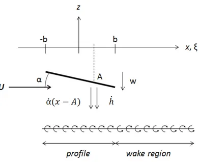
Figure 2.3-1Vortex model for a pitching flat-plate

projected on a line parallel to the flow, as shown in Fig. 2.3-1. The motion of the airfoil is then represented by a plunging component, ḣ and a pitching component α̇. The unsteady Bernoulli equation can be given as it follows.

∆𝑝(𝑥, 𝑡) = 𝜌 [𝑈∞(𝑡)𝛾(𝑥, 𝑡) +_{𝜕𝑡 ∫ 𝛾}𝜕 (𝜉, 𝑡)𝑑𝜉 𝑥

0 ]

(2.5)

Where



𝐿 = ∫ ∆𝑝(𝑥, 𝑡)𝑑𝑥𝑐

0 = 𝜌𝑈∞(𝑡) ∫ 𝛾(𝑥, 𝑡)𝑑𝑥

𝑐

0 + 𝜌

𝜕

𝜕𝑡 ∫ (𝑥 − 𝑐)𝛾(𝑥, 𝑡)𝑑𝑥

𝑐

0

(2.6)

The first term of the equation corresponds to the Kutta-Joukowski Theorem, being the integral the equation for the circulation Γ over the airfoil. The second part is the apparent mass effect, from the noncirculatory component of the flow. From the Biot-Savart Law, the downwash at z0 can be described as it follows, being a _{the vortex sheet strength at the profile and} w

the vortex sheet strength in the wake.

𝑤(𝑥, 0, 𝑡) = −_{2𝜋 ∫}1 +𝑏𝛾_{𝑥 − 𝜉 𝑑𝜉}𝑎(𝜉, 𝑡)

−𝑏 −

1 2𝜋 ∫

𝛾𝑤(𝜉, 𝑡)

𝑥 − 𝜉 𝑑𝜉

+𝑏

−𝑏

(2.7)

And from the analysis of the velocity components from Fig. 2.3-1, the downwash at the trailing edge can be written as:

𝑤 = 𝑈∞(𝑡)𝛼(𝑡) + ℎ̇(𝑡) + 𝛼̇(𝑡)(𝑥 − 𝐴) (2.8)

𝑤(𝑥, 𝑡) = 𝑤𝑎(𝑥, 𝑡) + 𝑤𝑤(𝑥, 𝑡) (2.9)

The flat-plate solution needs to satisfy the following conditions:

 The flow over the airfoil has to be tangent to its surface, hence the flow will not cross the airfoil wall, ensuring the Neumann Condition;

 The vorticity must be zero at the airfoil trailing edge, ensuring Kutta Condition, as the circulation Γ is such that the flow leaves the trailing edge smoothly;

 The total nonstationary circulation Γ is conserved, following Kelvin’s Circulation Theorem, whereD Dt0.

From the Kelvin’s Circulation Theorem is then possible to state that:

𝛤(𝑡) = 𝛤𝑎(𝑡) + 𝛤𝑤(𝑡) = 𝑐𝑡𝑒 (2.10)

From Neumann Condition, the vortex strength can now be represented considering:

𝑤(𝑥, 𝑡) − 𝑤𝑎(𝑥, 𝑡) − 𝑤𝑤(𝑥, 𝑡) = 0 (2.11)

𝑈∞(𝑡)𝛼(𝑡) + ℎ̇(𝑡) + 𝛼̇(𝑡)(𝑥 − 𝐴) − 𝑤𝑤(𝑥, 𝑡) = −_{2𝜋 ∫}1 𝛾_{𝑥 − 𝜉 𝑑𝜉}𝑎(𝜉, 𝑡) +𝑏

−𝑏

(2.12)

Applying the Kutta Condition at the trailing edge and considering mathematic operations it is possible to determine:

𝛾𝑎(+𝑏, 𝑡) = 0 (2.13)

𝛾𝑎(𝑥, 𝑡) = −2_𝜋√𝑏 − 𝑥_{𝑏 + 𝑥 ∫} √𝑏 − 𝜉_{𝑏 + 𝜉 .}𝑤𝑎(𝑥, 𝑡) − 𝑤_{𝑥 − 𝜉}𝑤(𝑥, 𝑡)𝑑𝜉 +𝑏

−𝑏

Theodorsen verified that the vorticity associated to flow circulation at the airfoil can be described as two components:

 The Circulatory Vorticity 𝛾_𝑎𝐶, which is the contributing component to the circulation Γ and has no effect over the downwash at the airfoil trailing edge;  The Noncirculatory Vorticity 𝛾_𝑎𝑁𝐶, under the conditions previously stated,

however does no contribute to Γ.

Hence, the lift can be found relating Eq. (2.6) and Eq. (2.14), being now divided in the components of the quasi stationary parcel, the induced lift parcel and the noncirculatory lift, as described in Eq. (2.15).

𝐿 = (𝐿𝑄𝑆+ 𝐿𝑊) + 𝐿𝑁𝐶 = 𝐿𝐶+ 𝐿𝑁𝐶 (2.15)

The terms of circulatory and noncirculatory lift are given as it follows:

𝐿𝑄𝑆 = 2𝜌𝜋𝑏𝑈∞(𝑡) [𝑈∞(𝑡)𝛼(𝑡) + ℎ̇(𝑡) + 𝛼̇(𝑡) (3𝑏_{2 − 𝐴)]} (2.16)

𝐿𝑊= 𝜌𝑈∞(𝑡) ∫ 𝑏

√𝜉2 _{− 𝑏}2 ∞

𝑏 𝛾𝑤(𝜉, 𝑡)𝑑𝜉 (2.17)

𝐿𝑁𝐶 = 𝜌𝜋𝑏2[𝑈∞(𝑡)𝛼̇(𝑡) + ℎ̈(𝑡) + 𝛼̈(𝑡)(𝑏 − 𝐴)] (2.18)

From Eq. (2.15) to (2.18) the lift over the airfoil can finally be written as described in Eq. (2.19).

𝐿(𝑡) =

∫ 𝜉

√𝜉2_{− 𝑏}2 ∞

𝑏 𝛾𝑤(𝜉, 𝑡)𝑑𝜉

∫ √𝜉 + 𝑏_𝑏∞ _{𝜉 − 𝑏}𝛾𝑤(𝜉, 𝑡)𝑑𝜉

Considering the harmonically plunging and pitching of the flat-plate, for the wake it is possible to consider:

𝜉̅ =𝜉_𝑏 (2.20)

𝛾𝑤(𝜉, 𝑡) = 𝛾̅𝑤𝑒𝑖(𝜔−𝑘𝜉̅) (2.21)

By substituting Eq. (2.21) in Eq. (2.19) is possible then to find the Theodorsen’s Function as a function of the reduced frequency of the flow.

𝐶(𝑘) =

∫ 𝜉̅

√𝜉̅2 _{− 1} ∞

1 𝑒−𝑖𝑘𝜉̅𝑑𝜉̅

∫ √∞ 𝜉̅ + 1⁄_{𝜉̅ − 1}𝑒−𝑖𝑘𝜉̅_𝑑𝜉̅ 1

(2.22)

Theodorsen identified the integrals as a combination of Hankel functions of second kind:

𝐶(𝑘) = 𝐻1(2)(𝑘)

𝐻₁(2)(𝑘) + 𝑖𝐻₀(2)(𝑘) (2.23)

Finally, the lift expression can be rearranged to a simple function of the Theodorsen’s function and the components of plunging and pitching of the airfoil, as described in the following equation.

𝐿(𝑡) = 𝜌𝜋𝑏2_[𝑈

∞(𝑡)𝛼̇(𝑡) + ℎ̈(𝑡) + 𝛼̈(𝑡)(𝑏 − 𝐴)]

+ 2𝜌𝜋𝑏𝑈∞(𝑡)𝐶(𝑘) [𝑈∞(𝑡)𝛼(𝑡) + ℎ̇(𝑡) + 𝛼̇(𝑡) (3𝑏_{2 − 𝐴)]}

(2.24)

𝐿(𝑡) = 𝜌𝜋𝑏2_[𝑈

∞(𝑡)𝛼̇(𝑡) + 𝛼̈(𝑡)(𝑏 − 𝐴)]

+ 2𝜌𝜋𝑏𝑈∞(𝑡)𝐶(𝑘) [𝑈∞(𝑡)𝛼(𝑡) + 𝛼̇(𝑡) (3𝑏_{2 − 𝐴)]}

(2.25)

The pitching lift coefficient can then be written as:

𝐶𝑙(𝑡) = _𝑈𝜋𝑏

∞2(𝑡)[𝑈∞(𝑡)𝛼̇(𝑡) + 𝛼̈(𝑡)(𝑏 − 𝐴)] +

2𝜋𝐶(𝑘)

𝑈∞(𝑡) [𝑈∞(𝑡)𝛼(𝑡) + 𝛼̇(𝑡) (

3𝑏

2 − 𝐴)] (2.26)

One can observe from Eq. (2.26) that the lift coefficient, as well for drag and pitching moment coefficients (not described in the analysis), depends on several parameters as the reduced frequency; free-stream velocity and the pitch derivatives, flow parameters as well as airfoil chord and the pitch axis position, geometric parameters. However, as the theory approaches the unsteady motion as a flat-plate pitching and plunging, the influence of the airfoil camber is not accounted. Thus, a different approach is necessary to model the unsteady motion of an airfoil. The influence of the reduced frequency and the pitch axis position on the pitching behavior is present on Fig. 2.3-2.

Figure 2.3-2Lift Coefficient curves from the Theodorsen’s function for a flat-plate in pure pitch motion. The hysteresis loop enlarges and moves down with the increase of the reduced frequency (left) and thins as the pitch axis

moves far from the leading edge (right)

6 8 10 12 14 16 18

0.2 0.4 0.6 0.8 1 1.2 1.4 1.6 1.8

Angle of Attack ()

L if t C o e ff ic ie n t - C l k=0.100 k=0.188 k=0.376

6 8 10 12 14 16 18

0.4 0.6 0.8 1 1.2 1.4 1.6 1.8

Angle of Attack ()

3

Goals

Although the Theodorsen’s function can explain the hysteretic behavior for the airfoil lift during an unsteady harmonic motion it cannot accounts for the rotational behavior of the fluid that can be encountered during unsteady motion. Also, the Theodorsen’s function is limited to low Reynolds numbers, differently from what aircraft and wind turbines can encounter during operation. Experimental analysis from ELDV measurements, as the study from Berton et al.

(2002), have shown that the downstroke phase for the harmonic pitching motion presents a tridimensional behavior, which is not accounted by the Theodorsen’s function as well. Hence, new methods are necessary to model flows closer to operational conditions, characterized by higher order Reynolds numbers and rotational behavior, as the flow is expected to be turbulent.

The purpose of this study is to model the pitching motion of a NACA 0012 airfoil and evaluate the capabilities of URANS k-ω SST model on modelling unsteady pitching flows, which is an approximation of the vibration that can be faced by aerodynamic bodies during flight, for different Reynolds numbers. The two-dimensional CFD computations here presented are based on the experimental studies from Berton et al. (2002) and McAlister et al. (1978), for Reynolds number 105 and 2.5x106, respectively.

4

Mathematical Modeling

From the literature review it is possible to understand that this kind of problem can be approached using many different schemes, from one and two equation models to higher order methods. However the complexity of this kind of flow requires an approach that is able to capture its characteristics, which can be difficult to model. Hence, once must choose a simulation technique that should model the problem with the necessary accuracy in an efficient way.

This chapter presents the mathematical modeling employed on the current study. The flow is modeled using the URANS method with the k-ω SST turbulence model, as will be detailed in the following sections.

4.1 Governing Equations

The incompressible Newtonian fluid flow can be described by the use of differential equations, where the flow is modeled by the Continuity and the Navier-Stokes Equations. These equations can be described as:

𝜕𝑢𝑖

𝜕𝑥𝑖 = 0

(4.1)

𝜕𝜌𝑢𝑖

𝜕𝑡 +

𝜕(𝜌𝑢𝑖𝑢𝑗)

𝜕𝑥𝑗 = −

𝜕𝑝 𝜕𝑥𝑗+

𝜕

𝜕𝑥𝑗[(𝜇 + 𝜇𝑡) (

𝜕𝑢𝑖

𝜕𝑥𝑗 +

𝜕𝑢𝑗

𝜕𝑥𝑖)] + 𝑓𝑖

(4.2)

The Continuity equation (Eq. 4.1) states that mass must be conserved through the boundaries of a control volume. The Navier-Stokes equation for momentum is described in Eq. (4.2).

4.2 The Unsteady Reynolds-averaged Navier-Stokes

demand time and great computational effort. One approach that can make good use of a less refined mesh and without consuming much computational effort is the unsteady RANS, often denoted URANS or Transient RANS, TRANS (Davidson, 2006, MTF270 Chalmers).

The technique uses a statistical, averaged, approach to approximate the Navier-Stokes equation, as proposed by Reynolds (1895). Time averaging is appropriate for stationary turbulence, as described by Wilcox (2006), which is a turbulent flow that, on the average, does not vary with time. The pitching flow is by definition unsteady; however, when considering a harmonic behavior of the pitch motion, it presents periodic characteristics that only can be modeled by an unsteady method. Hence the Unsteady RANS approach is suitable for the analysis.

Figure 4.2-1 Time averaging for stationary turbulence

As described by Reynolds, the instantaneous velocity field u_i(x, t) of the flow can be expressed as the sum of a mean velocity, U_i(x), and a fluctuating part, u_i′(x, t). This is known as Reynolds Decomposition.

𝑢𝑖(𝑥, 𝑡) = 𝑈𝑖(𝑥) + 𝑢𝑖′(𝑥, 𝑡) (4.3)

The mean velocity is denoted by:

𝑈𝑖(𝑥) = lim_{𝑇→∞𝑇 ∫ 𝑢}1 𝑖(𝑥, 𝑡)𝑑𝑡 𝑡+𝑇

𝑡

As one can expect, the time-average of the mean velocity is again the same mean velocity:

𝑈̅ (𝑥) = lim𝑖 _𝑇→∞1_{𝑇 ∫ 𝑈}𝑖(𝑥)𝑑𝑡 𝑡+𝑇

𝑡 = 𝑈𝑖(𝑥) lim𝑇→∞

1

𝑇 ∫ 𝑑𝑡

𝑡+𝑇

𝑡 = 𝑈𝑖(𝑥)

(4.5)

This leads to:

𝑢′𝑖

̅̅̅̅ = lim_{𝑇→∞𝑇 ∫}1 [𝑢𝑖(𝑥, 𝑡) − 𝑈𝑖(𝑥)]𝑑𝑡 𝑡+𝑇

𝑡 = 𝑈𝑖(𝑥) − 𝑈̅ (𝑥) = 0𝑖

(4.6)

Flows for which the mean flow contains very slow variations with time, as when it is necessary to compute the flow over a helicopter blade, for example, which can be described as a nonstationary turbulence flow.

Figure 4.2-2 Time averaging for nonstationary turbulence

To achieve a time varying approach, one must consider:

𝑢𝑖(𝑥, 𝑡) = 𝑈𝑖(𝑥, 𝑡) + 𝑢𝑖′(𝑥, 𝑡) (4.7)

𝑈𝑖(𝑥, 𝑡) = lim_{𝑇→∞𝑇 ∫ 𝑢}1 𝑖(𝑥, 𝑡)𝑑𝑡 𝑡+𝑇

𝑡

(4.8)

Which is the simplest approach, yet arbitrary. As stated before, the time-averaging of the fluctuations is still zero, thus, for any scalar p and vector u_i it is possible to write:

𝑝,𝑖

̅̅̅ = 𝑃,𝑖 & 𝑢̅̅̅̅ = 𝑈𝑖,𝑗 𝑖,𝑗 (4.9)

Yielding:

𝜕𝑢̅̅̅̅𝑖,𝑗

𝜕𝑡 = 𝜕𝑈𝑖,𝑗

𝜕𝑡 (4.10)

As stated by Wilcox (2006), the use of time-averaging is useful for the analysis, especially for steady flows. A degree of caution must be accounted when considering time-varying flows, though. This is mainly due to the fluctuations that are often in excess of 10% of the mean velocity of the flow. For the analysis of the Reynolds-averaged equations, Eq. (4.1) and Eq. (4.2), for incompressible flow, must be rewritten as:

𝜕𝑢𝑖

𝜕𝑥𝑖 = 0

(4.11)

𝜌𝜕𝑢_{𝜕𝑡 + 𝜌}𝑖 𝜕(𝑢_𝜕𝑥𝑖𝑢𝑗)

𝑗 = −

𝜕𝑝 𝜕𝑥𝑗 +

𝜕𝑡𝑗𝑖

𝜕𝑥𝑗

(4.12)

Where t_ij is the viscous stress tensor as it follows:

𝑡𝑖𝑗 = 2𝜇𝑠𝑖𝑗 (4.13)

𝑠𝑖𝑗 =1_{2 (}𝜕𝑢_𝜕𝑥𝑖

𝑗 +

𝜕𝑢𝑗

𝜕𝑥𝑖) (4.14)

Combining Eq. (4.12) through Eq. (4.14) brings the conservation form of the Navier-Stokes equations:

𝜌𝜕𝑢_{𝜕𝑡 + 𝜌}𝑖 𝜕(𝑢_𝜕𝑥𝑖𝑢𝑗)

𝑗 = −

𝜕𝑝 𝜕𝑥𝑗 +

𝜕(2𝜇𝑠𝑗𝑖)

𝜕𝑥𝑗

(4.15)

Applying the time-averaging to Eq. (4.11) and Eq. (4.15), considering also Eq. (4.9):

𝜕𝑈𝑖

𝜕𝑥𝑖 = 0

(4.16)

𝜌𝜕𝑈_{𝜕𝑡 + 𝜌}𝑖 𝜕(𝑈𝑖𝑈𝑗_𝜕𝑥− 𝑢̅̅̅̅̅̅)𝑖′𝑢𝑗′

𝑗 = −

𝜕𝑃 𝜕𝑥𝑗+

𝜕(2𝜇𝑠̅̅̅)𝑗𝑖

𝜕𝑥𝑗

(4.17)

Where by rearranging Eq. (4.17) it is possible to write the momentum equation in tensor notation, as it follows:

𝜕𝑈𝑖

𝜕𝑡 +

𝜕(𝑈𝑖𝑈𝑗)

𝜕𝑥𝑗 = −

1 𝜌

𝜕𝑃 𝜕𝑥𝑗+

𝜕 𝜕𝑥𝑗[𝜈 (

𝜕𝑢̅𝑖

𝜕𝑥𝑗 +

𝜕𝑢̅𝑗

𝜕𝑥𝑖) − 𝑢𝑖 ′_𝑢𝑗′

̅̅̅̅̅̅] (4.18)

The Reynolds-averaged Navier-Stokes equation is then described by Eq. (4.18). The term −u̅̅̅̅̅̅i′uj′ is also known as the Reynolds-stress tensor, τij, which has to be modeled in order to solve

4.3 The Closure Problem

To model turbulence it is necessary to find an approximation for the Reynolds-stress tensor. Boussinesq (1877) proposed a solution by assuming that the Reynolds-stresses are proportional to the velocity gradients of the mean-flow, analogous to the viscous stresses, yielding:

𝜏𝑖𝑗 = −𝑢̅̅̅̅̅̅ = −𝜈𝑖′𝑢𝑗′ 𝑡(𝜕𝑢_𝜕𝑥̅𝑖 𝑗+

𝜕𝑢̅𝑗

𝜕𝑥𝑖) +

2

3 𝑘𝛿𝑖𝑗 (4.19)

The kinetic energy 𝑘 and the kinematic Eddy viscosity 𝜈_𝑡 are unknown, since:

𝑘 =1_{2 𝑢}̅̅̅̅̅̅ = 1𝑖′𝑢𝑗′ _{2 (𝑢}̅̅̅̅ + 𝑣′2 ̅̅̅̅ + 𝑤′2 ̅̅̅̅̅)′2 (4.20)

And the kinematic Eddy viscosity is modeled by introducing extra equations. For RANS simulations two of the most used turbulence models are the k-ε and k-ω, where both solve two extra transport equations, one for k and one for ε or ω. The kinematic viscosity is modeled by the k-ε as:

𝜈𝑡= 𝐶𝜇𝑘 2

𝜀 (4.21)

and the k-ω as:

𝜈𝑡 =_𝜔𝑘 (4.22)

4.4 Turbulence Modeling

Aeronautical flows are surely a class where the prediction of its properties needs high accuracy, mainly due to strong adverse pressure gradients and separation in boundary layers. The k-ε and k-ω two-equation RANS models are not able to capture the proper behavior of turbulence in aeronautical flow. The popular k-ε can give a well-defined boundary layer-edge during simulation; however, it is less accurate and complex on sublayer modelling. The k-ω is substantially more accurate in the sublayer; yet it is sensitive in the freestream, which is the cause of the k-ε being the standard equation in turbulence modelling (Menter et al., 2013). Both standard two-equation models overpredict the shear stress in adverse pressure gradient flows, even when considering delayed separation. The Shear Stress Transport SST model (Menter, 1993) was developed due to the need of more accurate separation prediction for aeronautic flows. The k-ω SST model is a blend of a k-ω model, which is used near walls in the sublayer prediction, and a k-ε model, used to predict the flow in the freestream region. Thus, the model is fairly robust, since it can accurately predict the flow at both sublayer and boundary layer edge and works better at capturing recirculation regions by enforcing the Bradshaw Relation.

To blend the k-ε and k-ω models, it is necessary to transform the former into equations based on k and ω. This leads to the cross-diffusion term, defined in Eq. (4.23).

𝐷𝑤 = (1 − 𝐹1)𝜌_𝜎𝜔2 _𝜕𝑥𝜕𝑘 𝑖

𝜕𝜔

𝜕𝑥𝑖 (4.23)

The blending function for the model is defined, assuming value zero in the freestream region, activating the k-ε cross diffusion term, and switches to one in the boundary-layer zone, to assure accurate calculation by the use of the k-ω function.

𝐹1 = 𝑡𝑎𝑛ℎ {{min [max (_𝛽√𝑘_{∗𝜔𝑦 ,}500𝜈_{𝑦2𝜔 ) ,}4𝜌𝜎𝜔

2𝑘

𝐶𝐷𝑘𝜔𝑦2]}} (4.24)

𝐶𝐷𝑘𝜔 = max (2𝜌𝜎𝜔2 1 𝜔

𝜕𝑘 𝜕𝑥𝑖

𝜕𝜔 𝜕𝑥𝑖, 10

−10_{) (4.25)}

The SST Turbulence Kinect Energy function is given as shown in Eq. (4.26). The Dissipation Rate, combining both standard k-ε and k-ω models by the use of the cross-diffusion term and the blending function F1 is shown at Eq. (4.27), being both the equations of this class of RANS model.

𝜕(𝜌𝑘) 𝜕𝑡 +

𝜕(𝜌𝑈𝑖𝑘)

𝜕𝑥𝑖 = 𝑃̃𝑘− 𝛽

∗_{𝜌𝑘𝜔 +} 𝜕

𝜕𝑥𝑖[(𝜇 + 𝜎𝑘𝜇𝑡)

𝜕𝑘 𝜕𝑥𝑖]

(4.26)

𝜕(𝜌𝜔) 𝜕𝑡 +

𝜕(𝜌𝑈𝑖𝜔)

𝜕𝑥𝑖

= 𝛼𝜌𝑆2_{− 𝛽}∗_𝜌𝜔2₊ 𝜕

𝜕𝑥𝑖[(𝜇 + 𝜎𝜔𝜇𝑡)

𝜕𝜔

𝜕𝑥𝑖] + 2(1 − 𝐹1)𝜌𝜎𝜔2

1 𝜔 𝜕𝑘 𝜕𝑥𝑖 𝜕𝜔 𝜕𝑥𝑖 (4.27)

The turbulent Eddy viscosity is defined as:

𝜈𝑡 =_max[𝑎𝑎1𝑘

1𝜔, 𝑆𝐹2] (4.28)

Where S is the strain rate and F2 is a second blending function defined by Eq. (4.29). The model uses a production limiter to avoid turbulence build-up in stagnation regions, as Eq. (4.30).

𝐹2 = 𝑡𝑎𝑛ℎ {[max (_𝛽2√𝑘_{∗𝜔𝑦 ,}500𝜈_{𝑦2𝜔 )]} −2

} (4.29)

𝑃𝑘= 𝜇𝑡𝜕𝑈_𝜕𝑥𝑖 𝑗(

𝜕𝑈𝑖

𝜕𝑥𝑗 +

𝜕𝑈𝑗

𝜕𝑥𝑖) → 𝑃̃𝑘 = min(𝑃𝑘, 10𝛽

∗_{𝜌𝑘𝜔) (4.30)}

5

Numerical Setup

As stated in Chapter 3, the airfoil geometry for the numerical simulations is the NACA 0012, in accordance with the experiments from Martinat et al. (2002) and McAlister et al.

(1978), for chord length based Reynolds number 105 and 2.5x106, respectively. The airfoil will pitch at the quarter chord position aft the leading edge, also known as both center of pressure and aerodynamic center for symmetric airfoils, as presented in the Thin Airfoil Theory (Munk, 1922).

5.1 Physical Modelling

The pitching of the airfoil is governed by a time dependent sinusoidal equation that guarantees the oscillation of the angle of attack. As presented in by Berton et al. (2002) and McAlister et al. (1978) there is generation of a periodic hysteresis cycle when analyzing the aerodynamic coefficients as lift and drag. The governing equations of the selected pitching motion can be described by the following equation.

𝛼(𝑡) = 𝛼𝑚𝑖𝑛+ {[𝛼𝑚𝑎𝑥− 𝛼₂ 𝑚𝑖𝑛] [1 − cos(𝜔𝑡)]} (5.1)

Figure 5.1-1 Schematics for the NACA 0012 airfoil pitch motion

quarter-chord axis. In his work, it is shown that the hysteresis loop enlargement and the dynamic stall recovery is delayed as the reduced frequency, 𝑘 = 𝜔𝑐 2𝑈⁄ _∞, is increased; deviating from the static airfoil values for aerodynamic coefficients given as function of the incidence angle.

5.2 Computational Mesh

The mesh used for the calculations is a 69300 nodes quad cell C-Grid topology two-dimensional mesh and was refined to ensure a y+ less than one for both numerical analyses, using Reynolds number of 105 and 2.5x106. The computation domain extent being 20c upstream and 20c downstream the airfoil pitch axis, the inner circular domain has a 10c diameter and is centered at the pitch axis, located at 0.25c aft the leading edge. The mesh uses the Sliding Mesh concept to emulate the pitching motion of the airfoil, the concept is applied to avoid re-meshing and ensure that the cell quality is kept close to the wall.

Figure 5.2-1 C-Grid computational domain mesh (left); internal circular domain for sliding mesh (center) and mesh interface domain connection –‘hanging nodes’ (right)

The domain is composed by two sub-domains: the external domain, with 100 nodes in I

the cells during motion in the ongoing simulation. The grid refinement was performed only with quadrangular elements to achieve numerical stability in the simulations by a high quality mesh. The refinement was sufficient to achieve mesh-independent results.

The concept of Sliding Meshes is applied to the interfaces between the circular and external domain (Fig. 5.2-2), creating non-matching nodes due to the rotation, also known as ‘hanging nodes’. This maintains the accuracy of the flow prediction close to the wall. Since the nodes are supposed to have a steady position in reference to their moving frame, no smoothing dynamic mesh method is necessary and the quality does not change.

In order to avoid conservation problems the connecting walls between the domains are set as interfaces, so the fluid will flow without changes through it. This condition is set to keep the nodes and cell in the inner boundary of the external domain static, while the nodes and cells in the perimeter of the circular domain can slide following the pitching airfoil movement.

Figure 5.2-2 Sliding Meshes Concept applied to the internal circular domain for pitch motion

5.3 Procedure

𝛿𝛼̅=0.0250⁰; the next 5 cycles had 𝛿𝛼̅=0.0125⁰ and the last 5 cycles, 𝛿𝛼̅=0.00625⁰. The average pitch angle is defined in Eq. (5.2), where 𝑛_{𝑖𝑡𝑒𝑟𝑎𝑡𝑖𝑜𝑛𝑠} correspond to the number of iterations per cycle.

𝛿𝛼̅ = [_{𝑇 ∫ 𝛼}4 𝑇/2 (𝑡)𝑑𝑡

0 ] ∙

1 𝑛𝑖𝑡𝑒𝑟𝑎𝑡𝑖𝑜𝑛𝑠

(5.2)

The results analysis for aerodynamics coefficients showed that the computations achieve stability prior to the 10 first cycles; hence for the next 10 cycles there was only a small deviance between each cycle and the averaging. At the inlet of the domain the fluid is flowing in the I

direction with a turbulence intensity of 5% and turbulent viscosity ratio of 10. The airfoil walls were set with a no-slip condition and at the outlet the boundary condition was set to zero pressure gradient. Table 5.3-1 summarizes the flow properties for both simulation cases. To model the internal domain pitch an User Defined Function (ANSYS Fluent UDF) was created.

Table 5.3-1 Experiments conditions for the pitch motion and flow properties.

Experiment Berton et al. (2002) McAlister et al. (1978)

Reynolds Number 1.0 x 105 2.5 x 106

Minimum Incidence 6⁰ 5⁰

Maximum Incidence 18⁰ 25⁰

Reduced Frequency 0.188 0.100

Airfoil Chord 1.0 m 1.0 m

Time Stepping

0.025



0.0125



0.00625



Fluid Air Air

Fluid Density 1.225 kg/m3 1.225 kg/m3

Fluid Viscosity 1.7894 x 10-5 Pa.s 1.7894 x 10-5 Pa.s

Turbulence Intensity 5% 5%

6

Results and Analysis

The URANS simulations analysis employed the k-ω SST two-dimensional turbulence model to analyze the pitching motion presented on the studies of Berton et al. (2002) and McAlister et al. (1978). The first set of simulations was based on the Berton et al. studies for Reynolds number 105 and reduced frequency k = 0.188. The oscillation range was 6⁰ to 18⁰, mean incidence of 12⁰. The second set of simulation, based on the experiments from McAlister

et al., for Reynolds number of 2.5x106 and reduced frequency k = 0.100. The oscillating range was 5⁰ to 25⁰, mean incidence of 15⁰.

As commented in the previous sections, the analysis was based on the averaging of the last 5 cycles of 20 simulated pitching cycles. The time step was based on an average pitch step, which was refined from 𝛿𝛼̅=0.0500⁰ to 𝛿𝛼̅=0.003125⁰. For both Reynolds numbers the hysteresis loop presents a refined behavior for an average pitch step of 𝛿𝛼̅=0.00625⁰. Refining the pitch step beyond that, and consequently the time step, did not affect the behavior any further, and so forth would only result in increasing the computational effort. Hence, the average pitch step of 𝛿𝛼̅=0.00625⁰ was used for the last 5 cycles average analysis as it is possible to consider the solution time-step independent. The analysis is shown in Fig. 6-1.

6.1 Pitching Analysis at Reynolds Number 105

The simulation results using the k-ω SST model are compared with the experiments from Berton et al. (2002), the two-dimensional k-ε Chien from Martinat et al. (2008) and the LES model three-dimensional computations from Kasibhotla & Tafti (2014). However the flow approximation is underestimated for the lift computations during the upstroke phase (↑), the SST modelling provides a less critical prediction when compared with the LES during the downstroke (↓). Although the SST predicted upstroke phase behavior is underestimated; it is qualitatively close to the LES computation, which indicates that the lift coefficient is not affected by three-dimensional effects.

Figure 6.1-1 Hysteresis loops obtained with two-dimensional RANS k-ω SST analysis for lift and drag compared to experimental results from Berton et al. (2002); k-ε Chien turbulence model simulations from Martinat et al. (2008)

and LES simulations from Kasibhotla & Tafti (2014) and the application of Theodorsen’s Function (1934)

display high oscillation characteristics during the downstroke phase, showing that the model is not able to capture all the circulation of an oscillatory flow with this scale of complexity. Of course, a flow of such complex unsteadiness is not easy to model, as turbulence modelling can render misleading predictions.

Figure 6.1-2 Vorticity colored streamlines for the NACA0012 pitching airfoil at 105 Reynolds number for the k-ω SST turbulence model, upstroke (↑) and downstroke (↓) phases

close to 6⁰, when the new pitching cycle begins, and its intensity will be reduced until the flow is fully attached to the upper surface again at 7.2⁰ upstroke (↑). The reattachment process is then completed, leading to the latter recirculation zone formation as the vortex shedding displays a periodic behavior, in agreement with the simulations from Kasibhotla & Tafti (2014) and Martinat et al. (2008).

It is important to note the influence of the lower surface on the flow behavior during the downstroke phase. As the airfoil pitches down, not only the flow is detaching from the upper surface caused by the vortex shedding, yet the lower surface is acting, in the other direction, producing an upward force and hence reducing the lift. Since the airfoil is symmetric, both surfaces act on the aerodynamic forces generation as explained by the Coanda Effect. Due to its viscosity the fluid will bend around a body as it sticks on the surface (Anderson & Eberhardt, 2001). The difference of speed on the fluid parcels of the boundary layer leads to the creation of shear forces that attach the flow and force it to bend in the direction of the slower layer, which is close to the wall, hence the fluid try to wrap around the object. When the flow is reattached near 7⁰ downstroke (↓), the upper surface again bends the air down in the trailing edge, as expected for a positive attitude incidence.

The analysis of the velocity streamlines from the SST computations and the experimental flow velocity field close to the surface of the airfoil surface measured by the Embedded Laser Doppler Velocimetry (ELDV) technique from Berton et al. (2002) shows qualitative agreement between both, as observable in Fig. 6.1-3. As expected, due to its flow two-dimensional behavior the upstroke phase is well represented by the k-ω SST 2D modelling. During the upstroke is possible to observe the formation of the leading edge recirculation region at 14⁰ and at the trailing edge the start of the boundary layer separation, leading to the formation of a vortex that will grow until the airfoil reaches its dynamic stall condition. During the downstroke phase it is possible to observe a slight difference between experimental and computational streamlines, the recirculation region close to leading edge for 14⁰ is similar to the experiments; still, the vortex formation for 10⁰ seems larger for the numerical analysis.

agreement; notwithstanding, the overall flow behavior is fairly represented, leading to the conclusion that the SST model can serve as an important tool to the understanding of pitching flow behavior. Also, the loop behavior for the latest SST simulation is by some extent similar to the Wall Resolved LES.

Figure 6.1-3 Analysis of flow behavior for ELDV (Berton et al., 2002) and k-W SST Analysis for 10⁰ and 14⁰, upstroke (↑) and downstroke (↓) phases

6.2 Pitching Analysis at Reynolds Number 2.5x106

layer, which is expected to be fully turbulent for Reynolds number 2.5x106, thus the k-ω SST is capable of modelling the flow more precisely. The upstroke phase shows a quite close agreement with experimental data, however, the behavior of the flow for the downstroke phase is still complex to represent, as is possible to see that the lift loss at the beginning of the phase is delayed with respect to experimental data. As seen in the previous analysis, the SST computations also over predict lift, though to a lesser extent.

Figure 6.2-1 Hysteresis loops obtained with two-dimensional RANS k-ω SST analysis for lift and drag coefficients compared to experimental results from McAlister et al. (1978) and k-ε Chien turbulence model simulations from

Martinat et al. (2008) and the application of Theodorsen’s Function (1934)

When compared with the k-ε Chien computation from Martinat et al. (2008), the surge in the lift coefficient for the simulated k-ω SST is delayed; however the upstroke phase is more accurate with respect to the experimental analysis for both lift and drag coefficients. During the downstroke it is observable again a high order oscillatory profile, which leads to the same hypothesis from the Reynolds number 105 analysis, the flow characteristics is expected to be tridimensional for the phase, contrariwise, due to its almost linear behavior during the upstroke, the flow is fairly represented by the 2-D URANS analysis. Also, the SST model presents a less critical drag coefficient hysteresis loop, even though it overpredicts the drag at the upstroke maximum incidence.

recirculation region during the upstroke (Fig. 6.2-2); the trailing edge vortex follows a similar behavior since it starts its growth at high incidence angles and then moves upstream the wall, reaching its maximum intensity until it sheds away with the flow in the start of the downstroke phase.

Figure 6.2-2 Vorticity colored streamlines for the NACA0012 pitching airfoil at 2.5x106 Reynolds number for the

k-ω SST turbulence model, upstroke phase (↑)

vortex shedding from the surface will lead to the dynamic stall before the maximum incidence. However, in the k-ω SST numerical analysis the trailing edge vortex starts from 20⁰(↑), reaching the leading vortex up to 24⁰(↑). From 24⁰(↑) to 25⁰ smaller vortical structures begin to form as well as the main structure starts to shed from the wall and the airfoil reaches its dynamic stall condition. As for the downstroke phase (Fig. 6.2-3), it is possible to note how the flow interacts with the trailing edge vortex and also with the airfoil lower surface since the flow is bent upwards, showing again the importance of the Coanda Effect to the viscous fluid flow analysis. The airfoil remains in the dynamic stall condition mostly during all the downstroke, until approximately 12⁰(↓).

Figure 6.2-3 Vorticity colored streamlines for the NACA0012 pitching airfoil at 2.5x106 Reynolds number for the

At 11⁰(↓) the vortical structures are shed away in the flow and the boundary layer reattachment process begins close to 8⁰(↓). This is in agreement with the experiment results, where is possible to observe that the dynamic stall remains until 10⁰(↓). Up to 5⁰ the airfoil regains lift due to the boundary layer reattachment to the surface. From 6⁰(↓) to 5⁰ the flow is already fully attached to the surface, completing the pitching cycle. It is important to notice that, since the flow is more accelerated, the boundary layer reattachment process can occur more rapidly, still during the downstroke phase.

The analysis of the aerodynamic coefficients and streamlines for the pitching cycle has shown that the k-ω SST turbulence model capabilities on modelling unsteady flows improve as the Reynolds number increases. Although there are differences from the experiments, the flow is better represented at Reynolds 2.5x106 and the 2-D URANS vortex shedding analysis can render important insights at low computational cost on the understanding of pitching airfoils. It is worth noticing that as the Reynolds number increases, the flow is closer to the potential approximation for the upstroke phase, as the velocity field is nearly irrotational up to 17⁰(↑), as can be seen in Fig. 6.2-4. The boundary layer is highly energized due to the flow acceleration in the leading edge and it is kept thin and close to the surface. It is possible to treat the flow as inviscid and irrotational, since viscous effects are limited to the boundary layer.

Figure 6.2-4 Vorticity colored streamlines and velocity contour (0 to 80 m/s) for the NACA0012 pitching airfoil at 2.5x106 Reynolds number for the k-ω SST turbulence model; 5⁰, 11⁰ and 17⁰, upstroke phase (↑). Local maximum

velocity of 61.39, 78.71 and 113.67 m/s and global maximum velocity of 121.52 m/s

when using the Euler Method as a tool for the analysis of unstalled pitching airfoils. However, as shown in the previous analyses, this assumption is only valid for the upstroke phase before the generation of the leading and trailing edge vortices and the recirculation region close to the wall. As the vortex sheds, the flow becomes highly rotational and the Potential Flow Theory is no longer applicable.

From the analysis of the lift coefficient hysteresis loops for the Berton et al. (2002) and McAlister et al. (1978) experiments in comparison with Theodorsen’s function, as shown respectively by Fig. 6.1-1 and Fig. 6.2-1, it is possible to observe that the Potential Theory can be addressed with fair results for the upstroke phase. Although the Theodorsen’s Theory (1934) has its limitations, the upstroke phase matched the experimental results for low order Reynolds number, as the flow can be modelled as potential as shown by Fig. 6.2-4. The surge of lift encountered seen in both experimental and numerical results cannot be accounted by the Theodorsen’s Theory as well, as it is a consequence of the vortex residence at the airfoil upper surface at the end of upstroke phase, presenting a high energy profile due to flow acceleration and vorticity. As discussed, the downstroke phase has a highly rotational behavior as well, which is not accounted by the Theodorsen’s function; hence the hysteresis loops for the theory cannot model the flow, differing from the experimental and numerical results.

7

Conclusions

The k-ω SST model is capable of predicting the behavior of the flow around pitching airfoils, also considering that the mesh is sufficiently refined for achieving such results. In the computations for the Berton et al. case the difference between simulations and experiments is mainly due to the transitional behavior of the boundary layer. Consequently, the SST model is likely to face problems on the modeling of such flows. Although the LES simulations from Kasibhotla & Tafti (2014) show a better agreement with the upstroke phase, the SST simulations display a downstroke less deviant from the experiments. Qualitatively, the SST presents a loop that is close to the LES behavior, showing that the SST model can provide results of reasonable quality while saving computational effort.

The analysis of the McAlister et al. computational case hysteresis loop shows better agreement between numerical computations and experimental data. Although there is clearly an overprediction of lift and delay on the dynamic stall angle prediction, the hysteresis loop is qualitatively close to the experiment. It was also possible to confirm the quasi potential behavior during most of the upstroke phase.

The complexity of the vortex shedding during the downstroke is not well modeled by the two-dimensional URANS, since it strongly three-dimensional behavior is inherent. One can conclude that the k- SST is capable of predicting some of the characteristics of pitching flows, not yet fully, nevertheless leading to important insights, as the qualitative behavior matched the expected one.