www.atmos-chem-phys.net/6/5129/2006/ © Author(s) 2006. This work is licensed under a Creative Commons License.
Chemistry
and Physics
Characterization of on-road vehicle emissions in the Mexico City
Metropolitan Area using a mobile laboratory in chase and fleet
average measurement modes during the MCMA-2003 field
campaign
M. Zavala1, S. C. Herndon2, R. S. Slott1, E. J. Dunlea1,*, L. C. Marr1,**, J. H. Shorter2, M. Zahniser2, W. B. Knighton3, T. M. Rogers3, C. E. Kolb2, L. T. Molina1,4, and M. J. Molina1,***
1Department of Earth Atmospheric and Planetary Sciences, Massachusetts Institute of Technology, Cambridge, MA, USA 2Center for Atmospheric and Environmental Chemistry, Aerodyne Research Inc., Billerica, MA, USA
3Department of chemistry and Biochemistry, Montana State University, Bozeman, MT, USA 4Molina Center for Energy and the Environment, San Diego, CA, USA
*now at: Cooperative Institute for Research in Environmental Sciences, University of Colorado, Boulder, CO, USA **now at: Department of Civil and Environmental Engineering, Virginia Tech. Blacksburg, VA, USA
***now at: Department of Chemistry and Biochemistry, University of California, San Diego, USA Received: 30 January 2006 – Published in Atmos. Chem. Phys. Discuss.: 12 June 2006
Revised: 14 September 2006 – Accepted: 21 October 2006 – Published: 8 November 2006
Abstract. A mobile laboratory was used to measure on-road vehicle emission ratios during the MCMA-2003 field campaign held during the spring of 2003 in the Mexico City Metropolitan Area (MCMA). The measured emission ratios represent a sample of emissions of in-use vehicles under real world driving conditions for the MCMA. From the rel-ative amounts of NOxand selected VOC’s sampled, the re-sults indicate that the technique is capable of differentiating among vehicle categories and fuel type in real world driv-ing conditions. Emission ratios for NOx, NOy, NH3, H2CO, CH3CHO, and other selected volatile organic compounds (VOCs) are presented for chase sampled vehicles in the form of frequency distributions as well as estimates for the fleet av-eraged emissions. Our measurements of emission ratios for both CNG and gasoline powered “colectivos” (public trans-portation buses that are intensively used in the MCMA) indi-cate that – in a mole per mole basis – have significantly larger NOx and aldehydes emissions ratios as compared to other sampled vehicles in the MCMA. Similarly, ratios of selected VOCs and NOyshowed a strong dependence on traffic mode. These results are compared with the vehicle emissions inven-tory for the MCMA, other vehicle emissions measurements in the MCMA, and measurements of on-road emissions in U.S. cities. We estimate NOxemissions as 100 600±29 200 metric tons per year for light duty gasoline vehicles in the
Correspondence to:M. Zavala ([email protected])
MCMA for 2003. According to these results, annual NOx emissions estimated in the emissions inventory for this cate-gory are within the range of our estimated NOxannual emis-sions. Our estimates for motor vehicle emissions of benzene, toluene, formaldehyde, and acetaldehyde in the MCMA in-dicate these species are present in concentrations higher than previously reported. The high motor vehicle aldehyde emis-sions may have an impact on the photochemistry of urban areas.
1 Introduction
Emissions from mobile sources in megacities represent a ma-jor contribution to the degradation of air quality at local and regional scales. They contribute to a primary and secondary air pollutant burden that can threaten human health, damage ecosystems and influence climate (Molina and Molina, 2004; Molina et al., 2004).
that affect the variability in emissions across different vehi-cles types. These include factors that affect the internal com-bustion efficiency in the vehicle, and therefore its engine’s emission characteristics, such as engine type and size, fuel composition, and combustion temperature and pressure. The character and maintenance of fuel delivering and emission control systems (or lack thereof) significantly affect which engine emissions exit the tailpipe. Traffic modes, road con-ditions, vehicle maintenance practices, driving behavior and other vehicle operating conditions can significantly affect ve-hicle emissions (Popp et al., 1999). The influence of all these factors highlights the need for measurement techniques that capture real-world vehicle emissions to validate emission in-ventories.
Several techniques have been developed to measure ve-hicle emissions both in laboratory testing and in real world driving conditions. These include measurement techniques using chassis dynamometer studies (Whitfield et al., 1998; Yanowitz et al., 1999), traffic tunnel integration studies (Kirchstetter et al., 1999), cross-road remote-sensing studies at tunnels and other fixed sites (Bishop et al., 1989; Jim´enez et al., 2000; Schifler et al., 2005), and Portable Emission Measurement System (PEMS) methods (Cadle et al., 2002). Real-world driving emissions measurement techniques may differ from dynamometer based testing techniques in several ways. Carefully controlled, but limited environmental con-ditions and driving patterns are typically used in chassis dy-namometer studies and typically a relatively small number of vehicles are tested.
Real world emission measurement techniques typically sample a much larger number of vehicles, but may do so un-der a limited range of driving states. Tunnel studies sample hundreds to thousands of vehicles, but are typically limited to fleet average emission values, although some differentia-tion between light duty and heavy duty vehicle emissions can be obtained when data for tunnel tubes that exclude heavy duty vehicles are compared with comparable mixed traffic tunnel data. Remote sensing measurement techniques typi-cally sample emissions from vehicles with a wide range of ages, models, maintenance and operational histories, but the sampling time is relatively short (∼0.1 s) and the range of driving states sampled is usually limited. On-board or trailer mounted PEMS instrumentation can characterize some emis-sions over a full range of on-road driving states, but are typi-cally deployed on a small number of vehicles in any study. Detailed descriptions of these techniques and a review of their strengths and limitations for determining mobile emis-sion factors are given elsewhere (e.g. Wenzel et al., 2000). As mobile emission inventories should accurately represent real world vehicle fleets and driving conditions, on-road mea-surement techniques that interrogate a wide range of vehicles over a full complement of drive states can make important contributions to this goal.
In recent years, additional techniques for the measurement of vehicle emissions under real-world driving conditions
us-ing fast response measurements in on-road mobile laborato-ries have been applied in urban areas (Kittelson et al., 2000; Vogt et al., 2003; Kolb et al., 2004; Canagaratna et al., 2004; Herndon et al., 2005a, b; Shorter et al., 2005; Pirjola et al., 2004; Giechaskiel et al., 2005). In the chase technique, a mobile laboratory repeatedly samples the emissions of a tar-get vehicle. Our implementation of this technique makes use of the fast time response and high sensitivity of laser spec-troscopic instruments and other fast response trace gas mea-surement techniques for repeatedly intercepting and measur-ing the turbulent exhaust plume of the target vehicle. Similar to the traditional remote sensing studies, ratios of a given species to CO2, used as a tracer of combustion, are obtained during the analysis and the results indicate the number of molecules of the pollutants of interest per CO2 molecules emitted. In addition to the chase technique, which focuses on a series of selected individual vehicles within a given ve-hicular class, fleet average on-road emissions can be obtained by processing randomly intercepted vehicle plumes from sur-rounding traffic (both co-flowing and opposing lanes). In this fleet average mode, even merged plumes from multiple vehi-cles can be processed and included.
In this study, emission ratios for selected individual vehi-cles as well as fleet average fuel-use-based vehicle exhaust emissions from mobile laboratory data are deduced from on-road measurements. In the fleet average mode the mobile laboratory measured on-road ambient air mixed with emis-sions of the surrounding vehicles. Successful application of this method requires a large sample size of these mixed emis-sion periods and a sampling time long enough such that the number of sampled vehicles is large enough to include a rep-resentative number of high emitters. Care must also be taken to avoid situations where the intercepted plumes are domi-nated by a few nearby vehicles for significant portions of the sampling period. On the basis of the central limit theorem, the emission averages should then be normally distributed if the samples are unbiased and sufficiently large.
version of the mobile laboratory was used to make initial on-road measurements in Mexico City in order to develop vehi-cle exhaust measurement techniques and survey the emission levels of selected pollutants as well as their ambient back-ground concentrations.
The MCMA-2003 field campaign featured the use of a new mobile laboratory equipped with fast time response in-strumentation to measure the emissions from on-road, in use vehicles in the MCMA. This version of the mobile lab and the measurement modes used during MCMA-2003 have been detailed in Kolb et al. (2004). In this work we present the analysis of the emission ratios obtained with chase and fleet average measurement modes during the MCMA-2003 field campaign. We present the analysis of mobile emission ra-tios for NOx, NOy, NH3, H2CO, CH3CHO, and other se-lected VOCs for chase sampled vehicles and fleet averaged emissions. The results are compared with the corresponding emissions inventory for the MCMA, other vehicle emissions measurements in the MCMA, and measurements of on-road emissions in U.S. cities.
2 Experimental methods
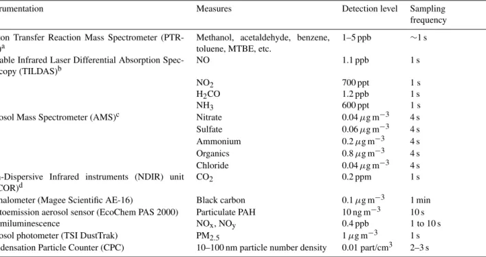
The mobile laboratory deployed during the MCMA-2003 field campaign was equipped with several high time resolu-tion and high sensitivity instruments (Kolb et al., 2004). As described in Table 1, these included Tunable Infrared Laser Differential Absorption Spectrometers (TILDAS) for mea-suring selected gaseous pollutants, a Proton Transfer Reac-tion Mass Spectrometry (PTR-MS) for measuring selected volatile organic compounds (VOCs), a commercial NO/NOy chemiluminescent detector modified for fast response mea-surements, and a Licor Non-Dispersive Infrared (NDIR) in-strument for CO2. Other inin-struments on board the mobile laboratory included a Global Positioning System (GPS), a sonic anemometer attached close to the laboratory sampling port to detect “tailwind” conditions that might create sampled air volumes contaminated with the mobile lab’s engine or on-board generator exhaust and a video camera used to obtain the target vehicle information. The mobile laboratory’s ve-locity and acceleration were measured and recorded contin-uously during the experiment along with local atmospheric parameters including pressure, temperature, and relative hu-midity.
VOCs emissions are of particular interest in this study; all the reported VOCs were measured with the PTR-MS sys-tem, except for H2CO that was measured with the TILDAS instrument. TILDAS instruments have been successfully em-ployed in several field campaigns for measuring trace gas species (Zahniser et al., 1995; Jim´enez et al., 1999, 2000) and for measuring emissions from passenger buses using the chase technique (Herndon et al., 2005a; Shorter et al., 2005). H2CO and NO2were measured using a lead salt tun-able diode lasers TILDAS instruments and NH3
measure-ments were obtained using a quantum cascade laser in the TILDAS system. The PTR-MS system (Ionicon Analytic GMBH) was applied for measuring vehicle emissions during on-road chase events for the first time during this study. It was used to measure selected oxygenated, olefinic, and aro-matic VOCs with proton affinities larger than water vapor via ionization through their reaction with H3O+. The resulting ions are detected by mass spectrometry at high time resolu-tion and selectivity. Data processing and validaresolu-tion meth-ods for VOCs measured with the PTR-MS system during the MCMA-2003 field campaign are reported in Rogers et al. (2006). NO and NOymeasurements were obtained with a chemiluminescent instrument using a molybdenum oxide converter modified for high frequency NOysampling (Dun-lea et al., 2004). Although in principle the measured NOy captures all reactive nitrogen oxides species, the contribution from reservoir and terminal species such as PAN, HNO3, and organic nitrates, is likely minimal to the overall fresh emitted NOy concentration due to the short time (few seconds) be-tween the emissions of NO and NO2and their sampling by the mobile laboratory.
Table 1.Instrumentation on board the Aerodyne mobile laboratory used during the MCMA 2002 and MCMA-2003.
Instrumentation Measures Detection level Sampling
frequency
Proton Transfer Reaction Mass Spectrometer (PTR-MS)a
Methanol, acetaldehyde, benzene, toluene, MTBE, etc.
1–5 ppb ∼1 s
Tunable Infrared Laser Differential Absorption Spec-troscopy (TILDAS)b
NO 1.1 ppb 1 s
NO2 700 ppt 1 s
H2CO 1.2 ppb 1 s
NH3 600 ppt 1 s
Aerosol Mass Spectrometer (AMS)c Nitrate 0.04µg m−3 4 s Sulfate 0.06µg m−3 4 s Ammonium 0.2µg m−3 4 s Organics 0.8µg m−3 4 s Chloride 0.04µg m−3 4 s Non-Dispersive Infrared instruments (NDIR) unit
(LICOR)d
CO2 0.2 ppm 1 s
Aethalometer (Magee Scientific AE-16) Black carbon 0.1µg m−3 1 min Photoemission aerosol sensor (EcoChem PAS 2000) Particulate PAH 10 ng m−3 10 s
Chemiluminescence NOx, NOy 0.4 ppb 1 to 10 s
Aerosol photometer (TSI DustTrak) PM2.5 1µg m−3 1 s Condensation Particle Counter (CPC) 10–100 nm particle number density 0.01 part/cm3 2–3 s
aOnly those components having proton affinities greater than water are detected using this technique which includes most oxygenated and
unsaturated hydrocarbons. bH
2CO was detected using a pair of absorptions lines at 1774.67 and 1774.83 cm−1. Two relatively weak water lines bracket these features, and a very small water line is present in the gap between. The diode used for NO2was operated at approximately 1606 cm−1and NO at approximately 1900 cm1. As operated during these measurements, the 1 s rms precisions for H2CO (diode 1) was normally less than 1.2 ppbv. For NO2(diode 2) the 1 s rms precision was 0.8 ppbv. NH3was operated with a quantum cascade laser at approximately 960 cm−1. cThe detection limits from individual species were determined by analyzing periods in which ambient filtered air was sampled and are
reported as three times the standard deviation of the measured mass concentration during those periods. dThe Licor-6262 non-dispersive infrared absorption instrument detects CO
2absorption in the 4.3µm band. Additional details regarding its performance in this application can be found elsewhere (Herndon et al., 2004). The measured response time of the Licor instrument to flooding the inlet tip with CO2free nitrogen gas during these experiments resulted in a 1/e time of 0.9 s.
The challenge then becomes to clearly distinguish between sampled emission exhaust and background concentrations, as well as to distinguish and discount emissions from other non-targeted vehicles. The identification of emission plumes from the data is accomplished by analyzing the multiple, syn-chronized, instruments on board the mobile laboratory. In addition to the pollutant sensors, these include 1) the read-ings from the sonic anemometer that allow consideration of the direction and speed of the incoming wind at the sam-pling port, 2) the images obtained with the video camera for observing the targeted vehicle, and 3) the real-time data log notes written by the researchers on-board the mobile labo-ratory. The use of these tools together with the analyses of the measured species signals are used to elucidate the pres-ence of background air and emissions related to the targeted vehicle. Similarly, the emissions from the mobile laboratory (vehicle exhaust plus generator exhaust) itself were flagged out in our database using the same discriminants described above, plus the fact that the generator emitted
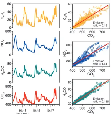
characteris-tic high levels of methanol. As described in Fig. 1, the sig-nals are correlated as long as they are part of the combustion products. When chasing a target vehicle, the instruments on board measure background and in-plume pollutant concen-trations and their correlation is obtained using CO2 as the combustion plume tracer. This technique is made possible by the high time resolution and sensitivity of the instrumen-tation that is capable of capturing and quantifying the rapidly changing emission concentrations.
Table 2.Chase and fleet average vehicle emissions experiments.
Event or chase type
Sample size MCMA fleet sizec Description
LDV 119 2 700 000 Fleet averaged emissions of Light Duty Vehiclesa HDT 61 75 000 Heavy Duty Trucks (e.g. heavy trucks, tractor trailers)
COL 71 32 000 Colectivosb
URB 37 30 000 Urban busesb
CHR 34 22 000 Inter-city buses or charters
Othersd 23 620 000 Includes combis, motorcycles, pickups, and non LDV vehicles≤3 tons
aIncludes events classified as SAG, “Stop and Go” (sampling size 12), TRA “Traffic state” (sampling size 19), and CRU, “cruising at high
speed” (sampling size 21), see text for details.
bColectivos are medium-size very popular public transport vehicles in the MCMA (for transporting about 25 people) powered by gasoline
fuel. Colectivos powered by CNG or LPG are denominated here as COLg (sampling size 26). Urban buses are intra-city diesel buses. See text for details.
cRounded values from the 2002 MCMA Emissions Inventory (SMA, 2004). Number of charters obtained from “Pasaje del Sevicio Publico
Federal de Autotransporte” in GDF (2000).
dFor our measurements, “Others” mean isolated emission plumes, fixed sampling or in specific places.
for light duty vehicles using the sampling periods when the mobile lab was surrounded by light duty gasoline vehicles under three different traffic conditions. We considered “Stop and Go” (SAG) situations when the mobile lab was in very heavy traffic conditions, with vehicle speeds lower than 16 (±8) km/h for 5 min or more. TRA events represent heavy traffic conditions with prevailing moderate speed, less than 40 (±16) km/h, for 5 or more minutes, this is the most preva-lent traffic mode in the MCMA. Finally, CRU conditions rep-resent sampling periods with prevailing cruising at moderate and high speed in the city, higher than 56 km/h, for 5 min or more. These traffic conditions accounted for 52 classified fleet averaged traffic mode events. As shown in Table 2, 67 other measurements of light duty gasoline vehicle emissions were considered but they were not classified within these cat-egories. In those cases, the classification was not possible ei-ther because the vehicle speed was not within a given vehicle speed category for more than 5 min (changing from one cat-egory to another, producing a combination of emission traf-fic modes) or because there was a strong influence from the emissions of an individual vehicle nearby (therefore biasing the fleet averaged sample).
Similar to the procedure used by Stedman et al. (1997), on the basis of the central limit theorem, the averaged emission ratios obtained should be approximately normally distributed if the samples were unbiased and sufficiently large. There-fore, the estimation of fleet average emission ratios with this method relies on the collection of average values represent-ing large, unbiased samples of fleet emission measurements of light duty vehicles surrounding the mobile lab. Heavy duty trucks and the other public transport vehicles that were indi-vidually sampled, as reported in Table 2, are intrinsically eas-ier to measure with the chasing technique due to the strength of their emission signal and to the ease of following them
800
600
400
CO
2
10:43 1/5/2003
10:45 10:47 800
400
0
NO
Y
80
40
0
H
2
CO
60
40
20
0
C
6
H
6
60
40
20
0
C
6
H
6
700 600 500 400
CO 2
600
400
200
NO
Y
700 600 500 400
CO 2
80
60
40
20
H
2
CO
700 600 500 400
CO 2
Emission ratio = 0.151
Emission ratio = 1.61
ratio = 0.185 Emission
Fig. 1.Time series of benzene, H2CO, and NOyin ppb units show-ing correlation with CO2in ppm units. Estimated emission ratios in right-hand panels are in ppb/ppm units.
2.1 Data processing procedure
The procedure for processing the data is described in the fol-lowing paragraphs. Consider the general case of a target ve-hicle whose concentration at the emission exhaust location is given byCie for a given speciesiwhileCiarepresents the ambient or background concentration for the same speciesi. In this way, the vehicle’s emission and background concen-trations for CO2would be given byCCO2e andCCO2a , respec-tively. Let the dilutionf be defined as the volume fraction of the exhaust plume for a given sampled volume in the mea-surement period (∼1 s). If the superscript m refers to the measured concentration:
f = C
m i −Cia
Cie−Cia. (1)
We can solve forCimas:
Cim=(1−f )Cia+f Cie. (2)
Iff=1, this implies that a pure exhaust is being measured and whenf=0, strictly ambient levels are being sampled. Now we make use of the equal dilution assumption for the species
iand for our tracer species CO2, from Eq. (1):
Cim−Cia
Cie−Cia =
CCO2m −CCO2a
CCO2e −CCO2a . (3)
We are interested measuring the emission ratio for the species
idefined in this context as:
ERi = C
e i
CCO2e . (4)
We can obtain this quantity from Eq. (3) after a series of simplifications. For example, with a typical concentration of CO2in an engine exit plume in excess of 2% and ambient levels generally below 400 ppm, the following approxima-tion is good to better than 2%.
CCO2e −CCO2a ∼=CCO2e . (5)
Similarly, for other species it is common to observe
Cia/Cievalues smaller than 0.05. Equation (4) simplifies to the intuitive expression,
ERi =
Cie
CCO2e
∼ = C
m i −C
a i
CCO2m −CaCO2. (6)
If the concentrationCimis plotted againstCmCO2a very simple diagnostic arises, which resembles a locus of points around the ambient concentrations ofiand CO2with rays extending toward higher concentrations of CO2when a plume is sam-pled. The slope of the correlation plot is indicative of the Emission Ratio for speciesi under the conditions in which the partially sampled plume was emitted.
3 Results
The measured emission ratios for the event types described above are shown in Table 3. Except for the fleet averaged light duty gasoline vehicles (SAG, TRA and CRU), the re-ported emission ratios correspond to the averaged values of the emissions from individual vehicle classes. Since the basis of the analytical procedure uses the covariance of the emit-ted species concentration to the emitemit-ted CO2concentration under an equal dilution assumption, and therefore avoiding having to resolve the highly transient plume dilution behav-ior, we have excluded emission ratios for species measured with the relatively lower sampling frequency instruments de-scribed in Table 1. In that way, we avoid the uncertainties resulting from correlating a low frequency signal with high frequency signals. An alternative approach to estimating fleet average emissions of pollutants measured with the slower re-sponse instrument instruments on-board the Aerodyne Mo-bile Laboratory during MCMA-2003, is presented by Jiang et al. (2005).
The video camera images were used during the analysis process to discriminate target vehicle plumes from other po-tential sources. During the chasing experiments, the target vehicle’s license plate was recorded so registration data could be accessed for additional information. The number of vehi-cles for which valid history information was available was too small to further classify the results by vehicle age and model.
Due to their large size, high exhaust volume, and relatively slow average speeds, public transport vehicles were sampled through individual chase events and were classified in this work as “colectivos” (COL), urban buses (URB), and char-ter buses (CHA). Colectivos are medium-size buses, with ca-pacity for transporting about 25 people, and are very popular and intensively used throughout the MCMA. Colectivos are mainly gasoline-powered, although a small but growing frac-tion of them (∼5%) are powered by CNG or LPG (CAM, 2004). By choosing a route used by colectivos fueled with CNG, we were able to sample 26 of this colectivo sub-class, classifying them as COLg. The URB category refers to intra-city urban buses with capaintra-city for transporting about 50 peo-ple; these buses were randomly selected as the mobile lab encountered them during on-road operations and a variety of transportation routes (and bus companies) were sampled. Charter buses, inter-city buses with a larger transport capac-ity than colectivos or urban buses, were sampled near the major bus terminal in the city. Here, the mobile lab chased the charter buses on a looped circuit as they were entering or leaving the facility. Sampled heavy-duty trucks (HDT) re-fer to large trucks such as tractor trailers, food supply and construction vehicles.
Table 3.Measured emission ratios in [ppb/ppm] during the MCMA-2003 field campaign.
Medium vehicles Light duty vehicles Heavy duty vehicles Pollutant COLd
(SD)c COLg (SD) LDV (SD) SAG (SD) TRA (SD) CRU (SD) URB (SD) CHR (SD) HDT (SD) NO 7.8 (3.0) 10.6 (4.1) 4.7 (2.4) 3.2 (1.0) 5.1 (2.0) 5.1 (1.6) 6.0 (1.5) 6.5 (1.9) 7.2 (3.0)
NO2 0.62
(0.4) 0.66 (0.32) 0.53 (0.45) 0.45 (0.42) 0.43 (0.33) 0.71 (0.30) 0.60 (0.26) 0.78 (0.33) 0.70 (0.35) NO 6.88 (3.4) 9.40 (3.8) 4.14 (2.4) 2.92 (0.9) 4.58 (2.2) 4.33 (1.7) 5.33 (1.6) 6.22 (1.9) 6.67 (3.2) H2CO 0.33
(0.12) 0.34 (0.13) 0.25 (0.11) 0.23 (0.06) 0.23 (0.07) 0.20 (0.07) 0.11 (0.07) 0.07 (0.05) 0.12 (0.08) CH3CO 0.04
(0.02) 0.06 (0.01) 0.04 (0.02) 0.04 (0.02) 0.04 (0.02) 0.04 (0.01) 0.02 (0.02) 0.02 (0.02) 0.03 (0.02) H2CO/CH3CHOa 8.1
(2.3) 6.4 (1.1) 6.7 (2.9) 6.2 (1.3) 6.2 (2.0) 6.4 (1.8) 7.2 (2.4) 4.9 (3.2) 5.1 (2.3) Benzene 0.08 (0.04) 0.03 (0.01) 0.13 (0.08) 0.14 (0.04) 0.10 (0.03) 0.10 (0.04) 0.04 (0.05) 0.02 (0.02) 0.03 (0.03) Toluene 0.14 (0.07) 0.04 (0.02) 0.25 (0.12) 0.28 (0.07) 0.18 (0.06) 0.18 (0.08) 0.05 (0.05) 0.02 (0.02) 0.04 (0.04) C2-Benzene 0.19 (0.09) 0.05 (0.04) 0.32 (0.16) 0.32 (0.11) 0.22 (0.09) 0.19 (0.09) 0.06 (0.06) 0.03 (0.04) 0.05 (0.05) C3-Benzene 0.16 (0.08) 0.03 (0.02) 0.24 (0.15) 0.24 (0.09) 0.15 (0.05) 0.15 (0.08) 0.05 (0.06) 0.03 (0.05) 0.05 (0.06)
m/z57e 0.26
(0.21) 0.03 (0.07) 0.38 (0.23) 0.39 (0.10) 0.29 (0.12) 0.28 (0.10) 0.09 (0.07) 0.04 (0.04) 0.09 (0.08)
NH3 NDc ND 0.12
(0.07) 0.09 (0.05) 0.09 (0.06) 0.11 (0.07) 0.04 (0.03) ND 0.06 (0.04) Aromatics/NOa,b 0.09
(0.08) 0.02 (0.01) 0.30 (0.27) 0.31 (0.10) 0.14 (0.07) 0.11 (0.05) 0.03 (0.03) 0.02 (0.02) 0.03 (0.03)
aObtained from individual emission ratios, see text for details, units in ppb/ppb.
bFor “aromatic VOCs” we considered the sum of Benzene, Toluene, C2-Benzene (sum of xylene isomers, ethylbenzene, and benzaldehyde)
and C3-Benzene (sum of C9H12isomers and C8H8O isomers). cSD: 1-standard deviation; ND: Non determined
dSee Table 2 and text for definition of vehicle chasses.
em/z57 represents the sum of MTBE and butenes for gasoline vehicles. Neutral components have not been assigned to this mass for CNG and diesel vehicles.
averaged ratios. In Fig. 2 we present the frequency distri-butions of measured emission ratios for various species and ratios of emitted species. The frequency distributions were obtained using all valid emission measurements for all the sampled species and vehicle categories. Similarly, frequency distributions for ratios of emitted species were also obtained from the ratios of individual, one-second, measurements.
4 Discussion
An important aspect of the analysis of the data collected is to determine how representative it is of the vehicle fleet emis-sions in the MCMA. Given the large population of the vehi-cle fleet, the presence of various driving modes and the vari-ability of all other parameters that play a role in the emission
30
20
10
0
Frequency,
%
20 15
10 5
0
NOY/CO2 , NO/CO2
3.0 2.0
1.0 0.0
NO2/CO2
NOY NO NO2
30
20
10
0
Frequency,
%
0.8 0.6
0.4 0.2
0.0
H2CO/CO2 , CH3CHO/CO2
30 20
10 0
H2CO/CH3CHO
HCHO CH3CHO HCHO/ CH3CHO
30
20
10
0
Frequency,
%
2.0 1.5
1.0 0.5
0.0
Benzene/CO2
0.8 0.6
0.4 0.2
0.0
Benzene/Toluene
Benzene Toluene Benzene/ Toluene
30
20
10
0
Frequency,
%
2.0 1.5
1.0 0.5
0.0
C2, C3_Benzene/CO2
4 3
2 1
0
Aromatic VOCs/CO2
C2Benzene C3Benzene Aromatics
40
20
0
Frequency,
%
2.0 1.5
1.0 0.5
0.0
(m/z57)/CO2
0.4 0.3
0.2 0.1
0.0
NH3/CO2
NH3
(m/z57)a
40
20
0
Frequency,
%
1.0
0.8
0.6
0.4
0.2
0.0
Aromatic VOCs/NO
YAro/NOY
Gasoline Aro/NOY
Diesel Aro/NOY
Fig. 2.Frequency distributions of measured emission ratios [ppb/ppm] during the MCMA.
a(m/z57)/CO
2represents MTBE + butenes for gasoline vehicles.
In this work, we have extended the analysis procedure for the chase technique by considering measurements for both fleet averaged and individual in-class vehicle emissions. As described above, we estimated fleet LDV average emissions by analyzing the sampling periods when the mobile labora-tory is measuring the mixed background air with the emis-sions of the surrounding vehicles for sustained periods of time. The assumption in this procedure is that the sampled emissions from a multitude of sources are sufficiently well mixed before arriving to the mobile lab sampling port. Since this condition is not totally controlled a priori for the experi-ment, it has to be determined from the analysis of the
emis-sion signals, the anemometer readings and the video camera. We have further classified such periods by driving state as SAG, TRA and CRU with the velocity criteria previously de-scribed. On the basis of the central limit theorem, the ob-tained fleet averages for each driving state should also be ap-proximately normally distributed if the samples are unbiased and sufficiently large. In such case, symmetric confidence intervals around the average could be established for fleet emissions estimates.
deviations that are significantly smaller than the observed av-eraged emission values. This is expected for fleet average estimates using the central limit theorem. NO2is a difficult species to measure with this technique due to its high reac-tivity and to potential ambient production via the reaction of NO with oxidizing species, such as ozone, that can be sig-nificant in a highly polluted atmosphere. In some cases, the sum of the NO and NO2emission ratios is greater than the NOyemission ratio. Although this is not physically possible for an individual vehicle, it may occur for the average values of groups of vehicles.
Due to the relatively small sample size and the lack of vehicle model year information, in the case of the individ-ual chase mode emission measurements of HDT and pub-lic transport vehicles the observed variability may not rep-resent the true variability of the population of emissions for these vehicle categories. The larger observed variability in these cases is likely the result of the large range of vehicles models, the variety of engine, fuel delivery, and emission control technologies, distribution of vehicle age and mainte-nance quality, and the variability of other parameters affect-ing emissions in real world drivaffect-ing conditions. As such, the averages and confidence intervals for these categories may not be representative of the entire fleet. Unless there is a sig-nificant increase of the sampling size, however, at this point the question of how much the obtained frequency distribu-tions would change by increasing the sampling size is un-solved.
In order to further reduce any systematic bias in the mea-sured emission ratios from individual chasing events reported in Table 3, during the experiment we intentionally did not fol-low a given vehicle class on the basis of the visible strength and blackness of its exhaust. That procedure helped to avoid over sampling of high emitting vehicles in the sampling pop-ulation. Similarly, since the mobile laboratory followed dif-ferent driving routes each day during the campaign through-out the city, the sampled emissions are most likely not biased by spatial differences in vehicle populations.
The obtained emission frequency distributions shown in Fig. 2 provide us with some interesting insights into the mo-bile emission characteristics in the MCMA. Different from a smoothed distribution, a pronounced cityscape type of graph may indicate the need for a larger sampling size population in our measurements. This is especially evident in the NH3 emission distribution, which was constructed from about 25% of the sample size for the other species. The smaller sample size for NH3was due to the need to divert a LiCOR CO2 instrument periodically to a shorter sampling inlet de-signed to avoid surface losses of NH3as well as some in-strumental problems characteristic of a first field deployment. Nevertheless, to our knowledge, this represents the first field deployment of a quantum cascade TILDAS on-board any mobile laboratory.
We define aromatic VOCs as the sum of benzene, toluene, C2-benzene (sum of xylene isomers, ethylbenzene, and
ben-zaldehyde) and C3-benzene (sum of C9H12 isomers and C8H8O isomers) as described in Rogers et al. (2006). Fig-ure 2 shows that these aromatic VOC/CO2 emission ratios tend to have higher frequency around a mean value but are also severely skewed towards high values of emission ratios. Although this behavior is often seen with VOC emission dis-tributions, we observe that the reported distributions of the ratios benzene/toluene and H2CO/CH3CHO tend to be nor-mally distributed, indicating the co-emission nature of these species in real world driving conditions.
The measured aromatic VOCs/NOy ratio presented in Fig. 2 shows a highly skewed but smoothly continuous hy-perbola type distribution. Since the detected aromatic VOC content of the emissions from the CNG colectivos are very low and close to the instrumental and analytical uncertainty, we have excluded them from the plotted aromatic species distributions. Therefore, an explanation for the behavior of the aromatic VOCs/NOy distribution may rely on the emis-sion characteristics of the vehicle fleet sampled (populations of vehicles with low versus high aromatic VOCs/NOy emis-sions) and on the fact that the two major fuel types, gaso-line and diesel, are included in the sample. To investigate which of these two aspects has a greater impact on the aro-matic VOCs/NOydistribution we included in Fig. 2 the cor-responding frequency distributions of gasoline and diesel ve-hicles that were sampled. The comparison of these distribu-tions reveals that within the gasoline vehicle fleet low and high emitting aromatic VOCs/NOy vehicles can be distin-guished. As long as the frequency distribution is represen-tative of the aromatic VOCs/NOy ratio in the vehicle fleet, this result has important implications for the design of air quality control strategies by allowing the possibility to direct air quality emission reduction strategies towards controlling the aromatic VOCs/NOyratio in different parts of the vehicle fleet and/or ranges of driving modes.
Public transport colectivos and buses are a very important part of the transport system in the MCMA (Gakenheimer et al., 2002). As an example, colectivos represent only about 1% of the vehicle fleet in the MCMA but, together with the other small popular public transport vehicle called “combis”, they account for almost 60% of the trips per person per day (CAM, 2004). Results presented in Table 3 indicate that, on a mole per mole basis, colectivos showed the highest NOx emissions ratios among the sampled vehicles, especially for colectivos fueled with CNG. The higher NOxemissions ra-tios for CNG colectivos is in accordance with their corre-sponding higher CH3CHO/H2CO ratio as compared to gaso-line fueled colectivos. The higher aldehyde emission ratios found in this work agree with dynamometer studies for CNG heavy duty vehicles performed by Huai et al. (2003) and Kado et al. (2005).
18
16
14
12
10
8
6
4
2
0
NO
X
/C
O2
, [ppb/ppm]
COL EI COLg EI LDV SAG TRA CRU EI Rf. a Rf. b Rf. c URB CHR HDT EI
(a) (b) (c)
COL COLg LDGV HDDT
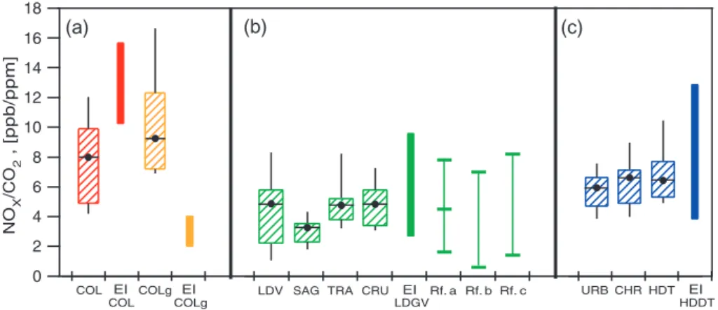
Fig. 3. Comparison of NOxemission factors obtained in this work (box plots) with estimates from the official 2002 MCMA Emissions Inventory (EI) (solid bars) and other studies (light lines) for panels:(a)colectivo buses,(b)Ligth duty Gasoline Vehicle (LDGV), and(c)
Heavy Duty Diesel Trucks (HDDT). Box plots represent the 10, 25, 75, and 90 percentiles along with the mean of our measurements. Filled bars represent the minimum and the maximum EI estimates for the corresponding vehicle category. Rf. a: Schifter et al. (2005); Rf. b: Schifter et al. (2004); Rf. c: Schifter et al. (2000).
aFor this comparison, we used fuel densities of 0.75, 0.85 and 0.41 kg/l for gasoline, diesel ad CNG fuels, respectively. Similarly, we
considered 70.3, 72.5 and 62.5 moles of C per kg of fuel for gasoline, diesel ad CNG, respectively. Fuel economies were assumed as follows: 10, 2.1 and 1.6 km/l for gasoline, diesel and CNG fleets, respectively.
may have important health implications. H2CO/CH3CHO ratios showed a value of 6.2±1.8 [ppb/ppb] averaged over all gasoline vehicle fleet emission measurements and the driv-ing mode did not significantly affect this ratio. Measured emissions indicate that the emitted species that are most in-fluenced by driving mode are NOx, aromatic VOCs and their aromatic VOCs/NOyratio. That effect was only investigated in the fleet average gasoline vehicle fleet and not in the indi-vidual chase emission measurements. As such, the observed variability within individual vehicle categories may be due to internal variability of the specific power of the vehicles, vehi-cle age and model, and emission control technology, among others. Nevertheless, the observed variability within driving modes for averaged vehicle fleet emissions indicates that this type of analysis for ratios of selected VOC to NOxspecies should be considered during the design of air quality control strategies that are based on the modification of the driving patterns, or modes, within the city.
An important aspect of this work lies in the comparison of the obtained results with the estimates for emission factors used in the official emissions inventory as well as with other measurements performed in the MCMA and other cities. The emissions inventory in the MCMA has been revised or updated every two years since 1994 and with homogenous methodologies since 1998. For comparisons with our re-sults, we use the 2002 official Emissions Inventory (EI) for the MCMA considering the categories of light duty vehicles, colectivos and heavy duty trucks for NOxemission factors. We present the comparison of our results with other estima-tions of emission factors in Fig. 3. The box plots represent the 10th percentile, 1st quartile, mean, 3rd quartile, and 90th
percentile of our measurements for each category whereas the thinner adjacent colored bars represent the range of emis-sion factors used in the emisemis-sions inventory. Light bars rep-resent the estimations of emission factors using other tech-niques. In order to compare the obtained emission ratios in ppb/ppm units with other measurements performed with different sampling techniques it is necessary to make use of fuel properties and stoichiometric combustion assumptions. Data considered for this purpose are presented in the notes for Fig. 3.
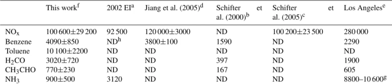
Table 4.Comparison of emissions (in tons/year) estimated in this work with emissions estimated in other studies for the MCMA and other U.S. cities.
This workf 2002 EIa Jiang et al. (2005)d Schifter et al. (2000)b
Schifter et al. (2005)c
Los Angelese
NOx 100 600±29 200 92 500 120 000±3000 ND 100 200±23 500 280 000
Benzene 4090±850 NDh 3800±100 1590 ND 2290
Toluene 10 100±2200 ND ND ND ND ND
H2CO 3020±720 ND ND 397 ND 1900
CH3CHO 770±230 ND ND 167 ND 605
NH3 900±500 3120 ND ND ND 8800–10 600g
aConsiders the emissions from the gasoline vehicle fleet: private vehicles, taxis, combis, colectivos and pickups. bBased on a laboratory study of around 50 vehicles (ages from 1984 to 1999) tested under a FTP cycle. cBased on a remote sensing study in 2000 for the MCMA.
dConsiders the total vehicle fleet, LDVs and HDVs.
eTotal on-road gasoline mobile emissions estimates for 2004 in the South Coast Air Basin. Source: CARB, 2005.
fUses gasoline fuel consumption by the transport sector alone estimated for 2002 in the MCMA Emissions Inventory and the fuel properties
reported in Fig. 3 of this document. gData includes all NH
3on-road mobile emissions taken from Fraser and Cass, 1998. hND: A value Non Determined in the study.
A similar comparison of our results with the NOxemission factors used in the MCMA emissions inventory for public transport vehicles indicates a possible overestimation in the gasoline-powered colectivos category. Similarly, our results indicate a possibly severe underestimation of NOxemission factors for CNG-powered colectivos. The emissions inven-tory uses the same NOx emission factors for our classified vehicle categories of URB, CHR and HDT, and their range falls within our results. However, in contrast to the com-parison with the light duty vehicle fleet, these results corre-spond to individual vehicle measurements and therefore the observed variability may or may not be representative of a given vehicle category. Note, however, that in the case of the CNG colectivos, the range estimated in the emissions in-ventory is too small compared to the range of the observed variability. Therefore, assuming that the observed variabil-ity is real, this may be indicative of a real underestimation of NOxemission factors used in the emissions inventory for this category.
The analysis of a possible under/over estimation of emis-sion factors is only a part of the validation of an emisemis-sions in-ventory. Since the emissions inventory is based on assumed values for activity parameters (e.g. distances traveled) that may introduce further uncertainty in the estimation of mo-bile emissions, the final estimation of emissions is not triv-ial. A possible way to circumvent this difficulty is to con-sider the use of fuel based emission factors together with es-timates of fuel consumption in a given region (Singer and Harley, 2000). We have followed this approach transforming our measured emission ratios to units of grams per unit of fuel consumed using the previously described assumptions of fuel properties and vehicle fuel efficiency. In the
transforma-tion of the emission factors we only considered the gasoline vehicle fleet averaged estimates.
Table 4 shows the comparison of our emission estimates for the MCMA with other studies. The results indicate that NOx emissions estimated for LDVs in the emissions inven-tory are within the range estimated using the fuel based emis-sion factors in this work of 100 600±29 200 metric tons per year. The upper and lower limits correspond to 1 standard deviation obtained from the observed emission factor for the LDV category. Although Table 4 shows that the comparisons for the total NOxemissions for light duty vehicles between the emission inventory and this work may be within the con-fidence intervals, the possible under/over estimation of emis-sion factors for individual vehicles ages and models may still be present in the emissions inventory. The application of the chase technique for systematically comparing emission fac-tors by vehicle age and model would then be desirable to address this question.
annual gasoline consumption was 3.3 times higher (Molina et al., 2004). Besides the larger size of the vehicle fleet and the corresponding higher fuel consumption in the Los Angeles area, two other important aspects of the comparison are the older vehicle fleet composition and the smaller fraction of vehicles with emission control technologies in the MCMA. For example, only about 30% of the vehicle fleet count with Tier (0 and 1) control emission technologies in the MCMA as compared to 91% in Los Angeles (Molina and Molina, 2002). This indicates that an aged vehicle fleet and a smaller fraction of vehicles with efficient emission control technolo-gies may have a significant impact on the overall burden of toxic VOC emissions in the MCMA. Bishop et al. (2001) has reported a slight but statistically significant increase of NO with increased altitude for heavy duty trucks. Nevertheless, reasons for the altitude relationship are unclear and may be subject to particular characteristics and composition of the sampled vehicle fleet.
As noted above, the sampling size of the measured on-road NH3 emissions was significantly smaller than the rest of the reported species due to the lack of a dedicated fast re-sponse CO2 monitor on the short, fast flow inlet necessary for NH3 measurements and some QC-TILDAS instrument problems characteristic of a first field deployment. As such, the NH3emission estimate in Table 4 has large confidence intervals and may not be fully representative of the LDV ve-hicle fleet. Nevertheless, the entire range estimate is signif-icantly smaller than the vehicle NH3emissions estimated in the current model based emissions inventory for the MCMA and than the on-road NH3 emission estimate in Los Ange-les. Given the median age of the MCMA vehicle fleet, this is not surprising since NH3emissions are dominated by newer gasoline powered vehicles equipped with NOxreduction cat-alysts. In our measurements, NH3 emissions for MCMA LDVs seem to be much higher for newer vehicles, which are presumably equipped with reduction catalysts for NOx and appear to be relatively independent of driving state. NH3 emitted from on-road vehicles may react rapidly with acid vapors to form high burdens of secondary particulate matter near heavily traveled roadways, impacting fine particle expo-sure levels for travelers and near by residents. The level of NH3emissions from newer LDV vehicles in the MCMA do appear to be significantly higher than the emissions of simi-lar vehicles in the U.S. (Herndon et al., 2005b). The impact of vehicular NH3 emissions on the MCMA NH3 emission inventory will be addressed more thoroughly in a separate publication (Shorter et al., 20061).
1Shorter, J. H., Herndon, S. C., Zahniser, M. S., et al.:
At-mospheric Ammonia in Mexico City during MCMA-2003, Atmos. Chem. Phys. Discuss., to be submitted, 2006.
5 Conclusions
In this work, we have extended the analysis procedure for the on-road mobile laboratory measurements by considering measurements of both fleet averaged emission measurements and individual vehicle emissions. The measured emission ra-tios represent a sample of emissions of in-use vehicles under real world driving conditions for the MCMA. From the rel-ative amounts of NOxand selected VOC’s sampled, the re-sults indicate that the technique is capable of differentiating among vehicle categories and fuel type in real world driving conditions. We have further classified our results by vehi-cle categories and driving mode using pre-established veloc-ity criteria in our analysis. Our measurements of emission ratios for both CNG and gasoline powered “colectivos” in-dicate that – in a mole per mole basis – have significantly larger NOx and aldehydes emissions ratios as compared to other sampled vehicles in the MCMA. Similarly, ratios of se-lected VOCs and NOyshowed a strong dependence on traffic mode. The potential implications of these results are impor-tant for the design of air quality control strategies based on the modification of the driving modes and the retrofitting of public transport vehicles.
By using a fuel consumption based approach together with the measured emission factors in this work, we estimate NOx emissions as 100 600±29 200 metric tons per year for LDGVs in the MCMA for 2003. According to these results, annual NOxemissions estimated in the emissions inventory for this category are within the range of our estimated NOx annual emissions. However, we did not explore the classi-fication of emissions by vehicle age and under/over estima-tions of NOxemissions for individual vehicle age categories can still exist in the emissions inventory. We also have esti-mated annual emissions for benzene, toluene, formaldehyde and acetaldehyde in the MCMA for the first time following a fuel-based procedure. The results indicate that the annual estimates of benzene, acetaldehyde and formaldehyde LDV emissions in the MCMA may be greater than previously re-ported and that their magnitudes are similar or higher than the corresponding estimated toxic VOC emissions in Los Ange-les and other U.S. cities. Vehicle age fleet composition and the relatively small fraction of vehicles with emission control technologies in the MCMA may significantly contribute for these large toxic emissions. Finally, ammonia emitted from newer reductive catalyst equipped LDVs may react rapidly with air vapors to form high burdens of secondary particu-late matter near heavily traveled roadways.
at MIT. We thank J. Sarmiento for providing the emissions in-ventory data and to N. Rodr´ıguez for the gasoline sales information.
Edited by: U. P¨oschl
References
GDF (Gobierno del Distrito Federal): Agenda estadistica del dis-trito federal-Transporte, Gobierno de M´exico, M´exico, available at http://www.df.gob.mx/agenda2000/, 2000.
Barnard, J. C., Kassianov, E. I., Ackerman, T. P., Frey, S., Johnson, K., Zuberi, B., Molina, L. T., Molina, M. J., Gaffney, J. S., and Marley, N. A.: Measurements of black carbon specific absorp-tion in the Mexico City Metropolitan Area during the MCMA 2003 field campaign, Atmos. Chem. Phys. Discuss., 5, 4083– 4113, 2005,
http://www.atmos-chem-phys-discuss.net/5/4083/2005/. Bishop, G. A., Starkey, J. R., Ihlenfeldt, A., Williams, W. J., and
Stedman, D. H.: IR long-path photometry: a remote sensing tool for automotive emissions, Analytical Chemistry, 61(10), 671– 677, 1989.
Bishop, G. A., Morris, J. A., Stedman, D. H., Cohen, L. H., Count-ess, R. J., CountCount-ess, S. J., Maly, P., and Scherer, S.: The effects of altitude on Heavy-Duty Diesel Truck on-road emissions, Env-iron. Sci. Technol., 35, 1574–1578, 2001.
Cadle, S. H., Gorse, R. A., Bailey, B. K., and Lawson, D. R.: Real-world vehicle emissions: a summary of the Eleventh Coordinat-ing Research Council On-Road Vehicle Emissions Workshop, J. Air Waste Manage. Assoc., 52(2), 220–236, 2002.
Canagaratna, M., Jayne, J., Ghertner, D., Herndon, S., Shi, Q., Jimenez, J., Silva, P., Williams, P., Lanni, T., Drewnick, F., De-merjian, K., Kolb, C., and Worsnop, D.: Chase studies of par-ticulate emissions from in-use New York City vehicles, Aerosol Sci. Technol., 38, 555–573, 2004.
CAM (Comisi´on Ambiental Metropolitana): Inventario de emi-siones 2002 de la Zona Metropolitana del Valle de M´exico, Sec-retar´ıa del Medio Ambiente, Gobierno de M´exico, M´exico, 2004. CARB, (California Air Resources Board): The California Almanac of Emissions and Air Quality – 2005 Edition, available at http: //www.arb.ca.gov/ei/emissiondata.htm, 2005.
de Foy, B., Caetano, E., Maga˜na, V., Zit´acuaro, A., C´ardenas, B., Retama, A., Ramos, R., Molina, L. T., and Molina, M. J.: Mexico City basin wind circulation during the MCMA-2003 field cam-paign, Atmos. Chem. Phys., 5, 2267–2288, 2005,
http://www.atmos-chem-phys.net/5/2267/2005/.
de Foy, B., Clappier, A., Molina, L. T., and Molina, M. J.: Distinct wind convergence patterns due to thermal and momentum forc-ing of the low level jet into the Mexico City basin, Atmos. Chem. Phys., 6, 1249–1265, 2006a.
de Foy, B., Varela, J. R., Molina, L. T., and Molina, M. J.: Rapid ventilation of the Mexico City basin and regional fate of the ur-ban plume, Atmos. Chem. Phys., 6, 2321–2335, 2006b. Dunlea, E., Volkamer, R., Johnson, K. S., Zavala, M., Molina, L. T.,
Molina, M. J., Lamb, B., Allwine, E., Rogers, T., Knighton, B., Grutter, M., Gaffney, J. S., Marley, N. A., Herndon, S. C., Zah-niser, M. S., Jayne, J., Shorter, J. H., Wormhoudt, J. C., and Kolb, C. E.: Nitrogen Oxides (NOy) in the Mexico City Metropolitan Area, American Geophysical Union, Fall Meeting 2004, abstract #A14A-05, 2004.
Fraser, M. P. and Cass, R. G.: Detection of excess ammonia emis-sions from in-use vehicles and the implications for fine particle control, Environ. Sci. Technol., 32, 1053–1057, 1998.
Gakenheimer, R., Molina, L. T., Sussman, J., Zegras, C., Howitt, A., Makler, J., Lacy, R., Slott, R. S., Villegas, A., Molina, M. J., and S´anchez, S.: The MCMA transportation system: Mobility and air pollution, in: Air Quality in the Mexico Megacity: An Integrated Assessment, edited by: Molina, L. T. and Molina, M. J., Kluwer Academic Publishers, Dordrecht, The Netherlands, pp. 213–284, 2002.
Garc´ıa, A., Volkamer, R., Molina, L. T., Molina, M. J., Samuelsson, J., Mellqvist, J., Galle, B., Herndon, S., and Kolb, C. E.: Separa-tion of emitted and photochemical formaldehyde in the Mexico City Metropolitan Area using a statistical analysis and a new pair of gas-phase tracers, Atmos. Chem. Phys., 6, 4545–4557, 2006, http://www.atmos-chem-phys.net/6/4545/2006/.
Giechaskiel, B., Ntziachristos, L., Samaras, Z., Scheer, V., Casati, R., and Vogt, R.: Formation potential of vehicle exhaust nucle-ation mode particles on-road and in the laboratory, Atmos. Envi-ron., 39, 3191–3198, 2005.
Herndon, S. C., Shorter, J. H., Zahniser, M. S., Wormhoudt, J., Nel-son, D. D., Demerjian, K. L., and Kolb, C. E.: Real-Time Mea-surements of SO2, H2CO, and CH4emissions from in-use curb-side passenger buses in New York City using a chase vehicle, Environ. Sci. Technol., 39, 7984–7990, 2005a.
Herndon, S. C., Jayne, J. T., Zahniser, M. S., Worsnop, D. R., Knighton, B., Alwine, E., Lamb, B. K., Zavala, M., Nelson, D. D., McManus, J. B., Shorter, J. H., Canagaratna, M. R., Onasch, T. B., and Kolb, C. E.: Characterization of urban pollutant emis-sion fluxes and ambient concentration distributions using a mo-bile laboratory with rapid response instrumentation, Faraday Dis-cuss., 130, 327–339, 2005b.
Herndon, S. C., Shorter, J. H., Zahniser, M. S., Nelson Jr., D. D., Jayne, J. T., Brown, R. C., Miake-Lye, R., Waitz, I., Silva P., Lanni, T., Demerjian, K. L., and Kolb, C. E.: NO and NO2 emis-sion ratios measured from in-use commercial aircraft during taxi and takeoff, Environ. Sci. Technol., 38(22), 6078–6084, 2004. Huai, T., Durbin, T. D., Rhee, S. H., and Norbeck, J. M.:
Investi-gation of emission rates of ammonia, nitrous oxide and other ex-haust compounds from alternative fuel vehicles using a chassis dynamometer, International Journal of Automotive Technology, 4(1), 9–19, 2003.
Jiang, M., Marr, L. C., Dunlea, E. J., Herndon, S. C., Jayne, J. T., Kolb, C. E., Knighton, W. B., Rogers, T. M., Zavala, M., Molina, L. T., and Molina, M. J.: Vehicle fleet emissions of black carbon, polycyclic aromatic hydrocarbons, and other pollutants measured by a mobile laboratory in Mexico City, Atmos. Chem. Phys., 5, 3377–3387, 2005,
http://www.atmos-chem-phys.net/5/3377/2005/.
Jim´enez, J. L., Nelson, D. D., Zahniser, M. S., Koplow, M. D., and Schmidt, S. E.: Characterization of on-road vehicle NO emis-sions by a TILDAS remote sensor, J. Air Waste Manage. Assoc., 49, 463–470, 1999.
Jim´enez, J. L., McManus, J. B., Shorter, J. H., Nelson, D. D., Zah-niser, M. S., Koplow, M., McRae, G. J., and Kolb, C. E.: Cross road and mobile tunable infrared laser measurements of nitrous oxide emissions from motor vehicles, Chemosphere – Global Change Science, 2, 397–412, 2000.
M. J., Cowin, J. P., Gaspar, D. J., Wang, C., and Laskin, A.: Processing of soot in an urban environment: case study from the Mexico City Metropolitan Area, Atmos. Chem. Phys., 5, 3033– 3043, 2005,
http://www.atmos-chem-phys.net/5/3033/2005/.
Kado, N. Y., Okamoto, R. A., Kuzmicky, P. A., Kobayashi, R., Ay-ala, A., Gebel, M. E., Rieger, P. L., Maddox, C., and Zafonte, L.: Emissions of toxic pollutants from compressed natural gas and low sulfur diesel-fueled heavy-duty transit buses tested over multiple driving cycles, Environ. Sci. Technol., 39(19), 7638– 7649, 2005.
Kirchstetter, T. W., Singer, B. C., Harley, R. A., Kendall, G. R., and Traverse, M.: Impact of California reformulated gasoline on motor vehicle emissions. 1. Mass emissions rates, Environ. Sci. Technol., 33, 318–328, 1999.
Kittelson, D., Johnson, J., Watts, W., Wei, Q., Drayton, M., Paulsen, D., and Bukowiecki, N.: Diesel Aerosol Sampling in the At-mosphere, Society of Automotive Engineers, paper number SAE 2000-01-2212, 2000.
Kolb, C. E., Herndon, S. C., McManus, J. B., Shorter, J. H., Zah-niser, M. S., Nelson, D. D., Jayne, J. T., Canagaratna, M. R., and Worsnop, D. R.: Mobile laboratory with rapid response instru-ments for real-time measureinstru-ments of urban and regional trace gas and particulate distributions and emission source characteristics, Environ. Sci. Technol., 38, 5694–5703, 2004.
Molina, M. J. and Molina, L. T.: Megacities and atmospheric pol-lution, J. Air Waste Manage. Assoc., 54(6), 644–680, 2004. Molina, L. T., Molina, M. J., Slott, R. S., Kolb, C. E., Gbor, P. K.,
Meng, F., Singh, R. B., Galvez, O., Sloan, J. J., Anderson, W. P., Tang, X. Y., Hu, M., Xie, S., Shao, M., Zhu, T., Zhang, Y. H., Gurjar, B. R., Artaxo, P. E., Oyola, P., Gramsch, E., Hidalgo, D., and Gertler, A. W.: Air quality in selected megacities, critical review complete online version, http://www.awma.org, 2004. Molina, L. T. and Molina, M. J.: Clearing the air: a comparative
study, in: Air Quality in the Mexico Megacity: An Integrated Assessment, edited by: Molina, L. T. and Molina, M. J., Kluwer Academic Publishers, Boston, 2002.
NARSTO, (North American Research Strategy for Tropospheric Ozone): Improving emissions inventories for effective air qual-ity management across North America, a NARSTO assessment, NARSTO-05-001, 2005.
Pirjola, L., Parviainen, H., Hussein, T., Valli, A., Hameri, K., Aaalto, P., Virtanen, A., Keskinen, J., Pakkanen, T.A., Makela, T., and Hillamo, R. E.: “Sniffer” – A Novel tool for chasing vehicles and measuring traffic pollutants, Atmos. Environ. 34, 3625–3635, 2004.
Popp, P. J., Bishop, G. A., and Stedman, D. H.: Development of a high-speed ultraviolet spectrometer for remote sensing of mobile source nitric oxide emissions, J. Air Waste Manage. Assoc., 49, 1463–1468, 1999.
Rogers, T. M., Grimsruda, E. P., Herndon, S. C., Jayne, J. T., Kolb, C. E., Allwine, E., Westberg, H., Lamb, B. K., Zavala, M., Molina, L. T., Molina, M. J., and Knighton, W. B.: On-road measurements of volatile organic compounds in the Mexico City Metropolitan Area using proton transfer reaction mass spectrom-etry, Int. J. Mass Spectr., 252(1), 26–37, 2006.
Salcedo, D., Onasch, T. B., Dzepina, K., Canagaratna, M. R., Zhang, Q., Huffman, J. A., DeCarlo, P. F., Jayne, J. T., Mor-timer, P., Worsnop, D. R., Kolb, C. E., Johnson, K. S., Zuberi,
B., Marr, L. C., Volkamer, R., Molina, L. T., Molina, M. J., Car-denas, B., Bernab´e, R. M., M´arquez, C., Gaffney, J. S., Marley, N. A., Laskin, A., Shutthanandan, V., Xie, Y., Brune, W., Lesher, R., Shirley, T., and Jimenez, J. L.: Characterization of ambient aerosols in Mexico City during the MCMA-2003 campaign with Aerosol Mass Spectrometry: results from the CENICA Super-site, Atmos. Chem. Phys., 6, 925–946, 2006,
http://www.atmos-chem-phys.net/6/925/2006/.
Schifter, I., D´ıaz, L., Mug´ıca, V., and L´opez-Salinas, E.: Fuel-based motor vehicle emission inventory for the metropolitan area of Mexico City, Atmos. Environ., 39, 931–940, 2005.
Schifter, I., D´ıaz, L., Vera, M., Guzm´an, E., and L´opez-Salinas, E.: Fuel formulation and vehicle exhaust emissions in Mexico, Fuel, 83, 2065–2074, 2004.
Schifter, I., D´ıaz, L., Vera, M., Castillo, M., Ramos, F., Avalos, S., and L´opez-Salinas, E.: Impact of engine technology on the vehicular emissions of Mexico City, Environ. Sci. Technol., 34, 2663–2667, 2000.
Shirley, T. R. , Brune, W. H., Ren, X., Mao, J., Lesher, R., Carde-nas, B., Volkamer, R., Molina, L. T., Molina, M. J., Lamb, B., Velasco, E., Jobson, T., and Alexander, M.: Atmospheric oxi-dation in the Mexico City Metropolitan Area (MCMA) during April 2003, Atmos. Chem. Phys., 6, 2753–2765, 2006,
http://www.atmos-chem-phys.net/6/2753/2006/.
Singer, B. C. and Harley, R. A.: A fuel-based inventory of motor ve-hicle exhaust emissions in the Los Angeles area during summer 1997, Atmos. Environ., 34, 1783–1795, 2000.
Shorter, J. H., Herndon, S., Zahniser, M. S., Nelson, D. D., Wormhoudt, J., Demerjian, K. L., and Kolb, C. E.: Real-time measurements of nitrogen oxide emissions from in-use New York City transit buses using a chase vehicle, Environ. Sci. Tech-nol., 39, 7991–8000, 2005.
Stedman, D. H., Bishop, G. A., Aldrete, P., and Slott, R. S.: On-road evaluation of an automobile emission test program, Environ. Sci. Technol., 31, 927–931, 1997.
Vogt, R., Scheer, V., Casati, R., and Benter, T.: O-road measurement of particle emission in the exhaust plume of a diesel passenger car, Environ. Sci. Technol., 37, 4070–4076, 2003.
Volkamer, R., Molina, L. T., Molina, M. J., Shirley, T., and Brune, W. H.: DOAS measurement of glyoxal as an indicator for fast VOC chemistry in urban air, Geophys. Res. Lett., 32, L08806, doi:10.1029/2005GL022616, 2005.
Wenzel, T., Singer, B. C., and Slott, R. S.: Some issues in the statis-tical analysis of vehicle emissions, Journal of Transportation and Statistics, September issue 1–14, 2000.
Whitfield, J. K. and Harris, D. B.: Comparison of heavy-duty diesel emissions from engine and chassis dynamometers and on-road testing, in: Eighth CRC On-Road Vehicle Emissions Workshop, San Diego, CA., Coordinating Research Council, 1998. Yanowitz, J., Graboski, M. S., Ryan, L. B., Alleman, T. L., and
Mccormick, R. L.: Chassis dynamometer study of emissions from 21 in-use heavy-duty diesel vehicles, Environ. Sci. Tech-nol., 33(2), 209–216, 1999.
![Table 3. Measured emission ratios in [ppb/ppm] during the MCMA-2003 field campaign.](https://thumb-eu.123doks.com/thumbv2/123dok_br/16384442.192178/7.892.109.786.130.632/table-measured-emission-ratios-ppb-mcma-field-campaign.webp)
![Fig. 2. Frequency distributions of measured emission ratios [ppb/ppm] during the MCMA.](https://thumb-eu.123doks.com/thumbv2/123dok_br/16384442.192178/8.892.147.751.87.774/fig-frequency-distributions-measured-emission-ratios-ppb-mcma.webp)