www.geosci-model-dev.net/8/911/2015/ doi:10.5194/gmd-8-911-2015
© Author(s) 2015. CC Attribution 3.0 License.
Description of algorithms for co-locating and comparing gridded
model data with remote-sensing observations
B. Langerock1, M. De Mazière1, F. Hendrick1, C. Vigouroux1, F. Desmet1, B. Dils1, and S. Niemeijer2
1Belgian institute for Space Aeronomy, Ringlaan 3, 1180 Ukkel, Belgium 2S&T, Olof Palmestraat 14, 2616 LR Delft, the Netherlands
Correspondence to:B. Langerock ([email protected])
Received: 29 September 2014 – Published in Geosci. Model Dev. Discuss.: 26 November 2014 Revised: 6 March 2015 – Accepted: 14 March 2015 – Published: 31 March 2015
Abstract. MACC-II,III, Monitoring Atmospheric Compo-sition and Climate, is the current pre-operational Coperni-cus Atmosphere Monitoring Service (CAMS). It provides data records on atmospheric composition for recent years, present conditions and forecasts (a few days ahead). To sup-port the quality assessment of the CAMS products, the EU FP7 project Network Of ground-based Remote-Sensing Ob-servations (NORS) created a server to validate the gridded MACC-II,III/CAMS model data against remote-sensing ob-servations from the Network for the Detection of Atmo-spheric Composition Change (NDACC), for a selected set of target species and pilot stations. This paper describes in detail the algorithms used in this validation server. Amongst others, the algorithms take into account the horizontal displacement of the measured profiles from the location of the instrument, the vertical averaging and uncertainty propagation.
1 Introduction and notations
MACC-III, Monitoring Atmospheric Composition and Cli-mate (http://copernicus-atmosphere.eu), is the current pre-operational Copernicus Atmosphere Monitoring Service (CAMS). It combines state-of-the-art atmospheric model-ing with Earth observation data to provide information ser-vices covering European air quality, global atmospheric com-position, climate forcing, the ozone layer and UV and so-lar energy, and emissions and surface fluxes. The EU FP7 R&D NORS project (Demonstration Network Of ground-based Remote-Sensing Observations in support of the Coper-nicus Atmospheric Service, http://nors.aeronomie.be) was set up to support the development and generation of
fit-for-purpose CAMS data products and services by providing quality information based on validation results. In NORS the validation will be carried out using NORS data prod-ucts which are essentially ground-based remote-sensing data from the Network for the Detection of Atmospheric Com-position Change (NDACC; see http://www.ndacc.org), opti-mized for the needs of the CAMS validation.
The validation processes carried out in NORS were cre-ated to be compliant with best practices as defined by the international community: all validation results include trace-ability information (see the Global Earth Observation System of Systems (GEOSS), Quality Assurance for Earth Observa-tion, QA4EO, 2010, and follow the validation road map for Copernicus atmospheric data and services formalized in the MACC validation protocol, Lambert, 2010; Huijnen and Es-kes, 2012). The validation support by NORS is delivered as a web-based application that generates default validation re-ports in an operational and automatic way, but which can also be used for the generation of dedicated user-driven validation reports on demand (http://nors-server.aeronomie.be).
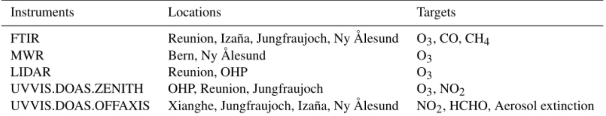
NORS is a demonstration project: it focuses on a limited number of target data products from a limited number of pi-lot NDACC stations representative of four major atmospheric regimes (Table 1).
MACC-Table 1. List of NORS pilot instruments, stations, and target parameters. UVVIS.DOAS.ZENITH (OFFAXIS) stands for UV–visible (MAX)differential optical absorption spectroscopy (DOAS), FTIR for Fourier transform infrared spectrometer and MWR for microwave radiometer.
Instruments Locations Targets
FTIR Reunion, Izaña, Jungfraujoch, Ny Ålesund O3, CO, CH4
MWR Bern, Ny Ålesund O3
LIDAR Reunion, OHP O3
UVVIS.DOAS.ZENITH OHP, Reunion, Jungfraujoch O3, NO2
UVVIS.DOAS.OFFAXIS Xianghe, Jungfraujoch, Izaña, Ny Ålesund NO2, HCHO, Aerosol extinction
II,III VAL is mostly using in situ surface data (AERONET, AErosol RObotic NETwork) or satellite total column data (e.g., Measurements of Pollution in the Troposphere (MO-PITT) and Infrared Atmospheric Sounding Interferometer (IASI) CO data), as reference data for the validation of the MACC-II,III products.
VAL produces 3 monthly validation reports for the near-real-time services of MACC-II,III, and 6 monthly valida-tion reports (updates) for the reanalysis services of MACC-II,III (http://www.copernicus-atmosphere.eu/services/aqac/ global_verification/validation_reports). The results of the NORS validation server have been used in the most recent VAL reports and in the latest reanalysis report.
The paper is organized as follows: in Sect. 2 a brief de-scription of the measurement and model data is presented. For the measurements, the basic GEOMS (Generic Earth Ob-servation Metadata Standard, Retscher et al., 2011) variables and their notations are introduced. For the model data, the al-gorithms to set up a vertical height grid and to do unit conver-sions are outlined. Section 3 contains the essential steps for comparing a single measurement with a model output. It de-scribes the re-gridding, temporal and spatial co-location and smoothing algorithms for model vertical profile data. Sec-tion 4 contains further details on how the validaSec-tion results are presented in their final output, e.g., time averaging of col-umn data or uncertainty propagation.
Regarding notation conventions, all multiplications are scalar; matrix multiplication is denoted by a central dot ·. Most of the notations used in the algorithms can be found in Tables 2, 3 and A1. For example, the profile array OM3 is linked to the MACC parameter go3 and denotes a target species vertical profile. To distinguish between the MACC and NORS vertical profile, a superscript notation is used, e.g., OM3 is the MACC model profile andON3 is the NORS measurement profile. If it is clear from the context to what class a data array belongs (model or measurement), the su-perscript is omitted to ease the notation.
2 Description of NORS and MACC data
2.1 NORS data
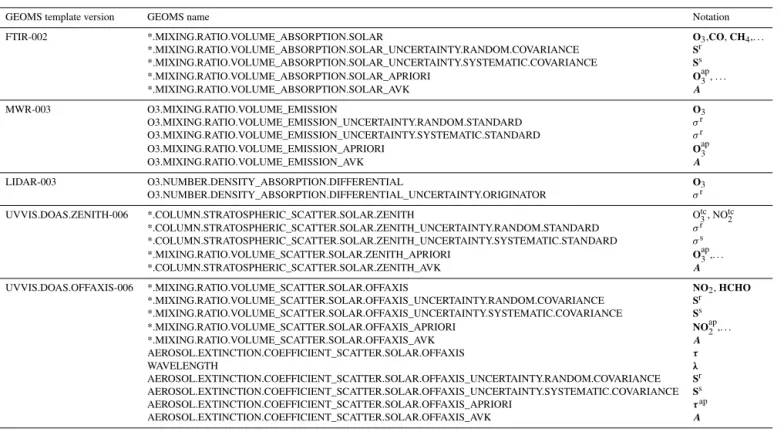
NORS data files are delivered in rapid delivery mode (not later than 1 month after acquisition) to the NDACC database rapid delivery directory, if not fully in final form, or to the corresponding NDACC database station directory if in its fi-nal form both with respect to data versioning (PI reviewed vs. operational) and file temporal coverage. For each measure-ment technique the NDACC data format has to be compliant with a pre-defined template (see http://avdc.gsfc.nasa.gov). The mapping of the template variable names to the mathe-matical concepts used throughout this paper, e.g., the target profile, the averaging kernel (AVK), is depicted in Table A1. Table 2 lists the GEOMS variables that all templates have in common (the dimensions are exemplary). All measurement techniques, except LIDAR, report averaging kernels, a priori profiles and uncertainties.
For each measurement technique, site and target species, a specific sensitivity range can be determined. For further details on sensitivity ranges and typical AVK’s, see the data user document that was developed within the framework of the NORS project (De Mazière et al., 2013).
2.2 MACC data
At present, the validation server validates in opera-tional mode the following forecast runs: near-real-time operation suite (NRT o-suite), the experiment running the TM5 3D atmospheric chemistry-transport model and the experiment with MOZART chemistry (for further details see https://www.gmes-atmosphere.eu/oper_info/nrt_ info_for_users, http://tm.knmi.nl). The model data are gener-ated regularly on specificoutput timesto(every 12 h for NRT
res-Table 2.List of GEOMS variable names common for all GEOMS templates (dimensions are indicative for 100 measurements on a grid with 47 layers).
Variable Dimension Unit Description Notation
DATETIME (100) s measurement time t
LATITUDE.INSTRUMENT (1) rad latitude of the instrument ϕ
LONGITUDE.INSTRUMENT (1) rad longitude of the instrument λ
ALTITUDE.INSTRUMENT (1) m altitude of the instrument zinst
ALTITUDE (47) m altitude grid (always descending) z
TEMPERATURE_INDEPENDENT (100, 47) K temperature profile T
PRESSURE_INDEPENDENT (100, 47) Pa pressure profile p
LATITUDE (100, 47) rad latitude of the location of probed air mass at each altitude (optional) λ
LONGITUDE (100, 47) rad longitude of the location of probed air mass at each altitude (optional) ϕ
ALTITUDE.BOUNDARIES (2, 47) m boundaries of vertical grid layers (optional) zB
Table 3. MACC variables specifications. MMR is mass mixing ratio. The dimensions are indicative for a model with IFS resolution T255N128.
Species Dimension Unit Description Notation
lnsp (256, 512) ln Pa logarithmic surface pressure (depends on latitude and longi-tude)
lnsp
– (61) Pa array ap contains the translation terms for the construction of the pressure grid
ap
– (61) – array bp contains the scaling factors in the construction of the pressure grid
bp
– (512) rad the array of longitudes (iλdenotes the index for this array) λ
– (256) rad the array of latitudes (iϕdenotes the index) ϕ
t (60, 256, 512) K temperature T
z (256, 512) m geopotential height of the surface (corresponds to lnsp) zs
q (60, 256, 512) kg kg−1 water vapor MMR (w.r.t. moist air) q go3 (60, 256, 512) kg kg−1 MACC ozone MMR (w.r.t. moist air) O3 hcho (60, 256, 512) kg kg−1 formaldehyde MMR (w.r.t. moist air) HCHO
co (60, 256, 512) kg kg−1 CO MMR (w.r.t. moist air) CO
aergn04 (60, 256, 512) – profile of aerosol optical depths at 532 nm τ532 aergn03 (60, 256, 512) – aerosol total optical depth at different wavelengths; each level
contains the total optical depth at different wavelengths: e.g., level 1 at 550 nm, level 2 at 340 nm, level 3 at 355 nm, level 4 at 380 nm–level 7 at 469 nm, level 9 532 nm
OD
ch4 (60, 256, 512) kg kg−1 CH4MMR (w.r.t. moist air) CH4 no2 (60, 256, 512) kg kg−1 NO2MMR (w.r.t. moist air) NO2
olutions1on regular Gaussian grids: T255N128 for NRT
o-suite and T159N80 for the other models.
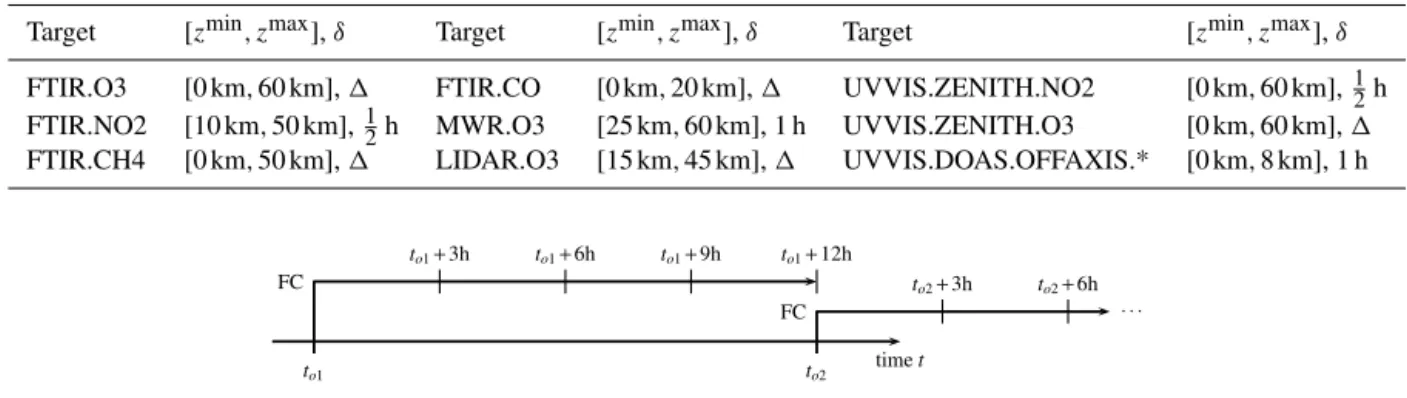
For each of these experiment versions, the validation server generates a time sequence of MACC model data with a time interval of 3 h between two MACC output times (see Fig. 1) such that the forecast validity times are as close as possible to the corresponding output times.
Table 3 describes the MACC data fields that are used in the validation server. The first column gives the MARS short
1An IFS resolution is denoted by TxNy:xindicates the spectral truncation andyis the number of latitudes between a pole and the
equator (for regular Gaussian grids, the number of longitude bands is 4y).
name or the parameter id. The dimension column is only in-dicative (these values change when considering other model grids. For notational convenience we fix the dimensions to the grid N128). Table 3 shows the notations of the MACC variable as they will appear in the algorithms.
The surface height variable zs [m] is the geopotential
Table 4.List of defaultzmin, zmaxvalues for NORS target species, based upon the measurement’s sensitivity range and upper boundaries of
MACC models, and of time windows for temporal co-location, based on species temporal variability.1is the time between two subsequent
MACC data validity times – see text (target values may contain wildcards if applicable to multiple targets).
Target [zmin, zmax],δ Target [zmin, zmax],δ Target [zmin, zmax],δ
FTIR.O3 [0 km,60 km],1 FTIR.CO [0 km,20 km],1 UVVIS.ZENITH.NO2 [0 km,60 km],12h
FTIR.NO2 [10 km,50 km],12h MWR.O3 [25 km,60 km], 1 h UVVIS.ZENITH.O3 [0 km,60 km],1
FTIR.CH4 [0 km,50 km],1 LIDAR.O3 [15 km,45 km],1 UVVIS.DOAS.OFFAXIS.* [0 km,8 km], 1 h
timet
FC
to1+3h to1+6h to1+9h to1+12h
FC · · ·
to2+3h to2+6h
to1 to2
Figure 1.Construction of MACC data times for type FC (forecast).
2.3 Vertical height grid for MACC data
This section contains a detailed description of the calculation of a vertical height grid for MACC data, starting from the vertical pressure coordinate. The algorithm described here calculates directly the height coordinate for the model pres-sure levels (i.e., the middle of a layer) and not for the prespres-sure interfaces (layer boundaries) of the model as it is described in the IFS documentation. Throughout this documentiϕ
de-notes the index for the longitude dimension, iλ the latitude
andithe vertical dimension.
Algorithm. (Pressure grid) Following the standard ECMWF procedure, the vertical pressure coordinatepis set up in the following way: the surface pressurepsequals
ps(iϕ, iλ)=elnsp(iϕ,iλ),
and the pressure on the level boundaries is
p(i, iϕ, iλ)=ap(i)+bp(i)ps(iϕ, iλ).
The pressurepis increasing in the vertical, i.e.,p(61,·,·)
corresponds to the surface pressure ps and p(1,·,·) is the
pressure at the top of the atmosphere. The vertical pressure coordinate on model levels then equals
pm(i, iϕ, iλ)=
1
2 p(i+1, iϕ, iλ)+p(i, iϕ, iλ)
.
All profile data (for the MARS variables go3, co, ch4, etc., except aergn03) are defined on model pressure levelspm.
To construct a vertical height vector out of the pressure grid, the server calculates the molar mass of humid air.
Algorithm. (Relative humidity) LetMX denote the
mo-lar mass of speciesX. By definition, the valueq(i, iϕ, iλ)is
the fraction MH2OnH2O
Mana wherenH2Orepresents the number of
molecules of water vapor in na molecules of air (na is the
number of molecules in theith layer at heightpm(i, iϕ, iλ)).
Similarly, nda denotes the number of particles dry air in
namol molecules air. Using the fact thatna=nda+nH2Oand
Mana=Mdanda+MH2OnH2O, it follows Mana=Mdana+
(MH2O−Mda)nH2O, or after division byMana:
1=Mda
Ma +
1− Mda
MH2O
q(i, iϕ, iλ).
In the next algorithm, we use the fractionMda/Ma
explic-itly:
Mda
Ma =1+
R
H2O
Rda −1
q(i, iϕ, iλ),
with Mda=28.960 g mol−1, MH2O=18.015 g mol−1, and
RdaandRH2Othe gas constants for dry air and water vapor,
respectively. For unit conversion algorithms, the molar mass of humid airMa(g mol−1) at the grid point(i, iϕ, iλ)is used
explicitly:
Ma(i, iϕ, iλ)=
MdaMH2O
MH2O(1−q(i, iϕ, iλ))+q(i, iϕ, iλ)Mda
.
Algorithm. (Height grid) We use the MACC pressure and temperature to construct a height coordinate in the usual way: we start with zs and construct recursively a height
for the upper levels using the hydrostatic balance equation
gMadz= −RTdln(p)(see Andrews, 2010). The latter
equa-tion is rewritten using the virtual temperature gMdadz=
−RTνdln(p), with
Tν=
Mda
MaT =T
1+
R
H2O
Rda −1
q
Earth accelerationgis approximated using WGS-84 (NIMA,
1984)g84(ϕ,z):
z(60, iϕ, iλ)−zs(iϕ, iλ)=
RdaTν(60, iϕ, iλ)
g84(ϕ(iϕ),zs(iϕ, iλ))
ln ps(iϕ, iλ)
pm(60, iϕ, iλ)
,
and recursively fori=59, . . .,1:
z(i, iϕ, iλ)−z(i+1, iϕ, iλ)=
RdaTν(i, iϕ, iλ)
g84(ϕ(iϕ),z(i+1, iϕ, iλ))
lnpm(i+1, iϕ, iλ)
pm(i, iϕ, iλ)
,
with Tν(i, iϕ, iλ)=12(Tν(i+1, iϕ, iλ)+Tν(i, iϕ, iλ)). The
validation server requires the knowledge of the thickness of the layers for re-gridding purposes. The heights of these boundaries of the layers do not match the MACC pressure grid p boundaries. Because these boundaries will only be used for re-gridding purposes, we believe that the differences that this approach may imply are negligible.
Algorithm. (MACC boundaries) The boundary height vec-tor zB at a chosen grid point (iϕ, iλ), consists of a lower
boundaryzB(1, i)and an upper boundaryzB(2, i)for theith
layer. The layer boundaries are calculated as the midpoints between layers, i.e., for i=1, . . .,59 (recall thatz denotes the decreasing MACC grid height vector):
zB(1, i)=1
2(z(i)+z(i+1)) zB(2, i+1)=zB(1, i).
The outer boundaries are determined from
zB(2,1)=z(1)+1
2|z(2)−z(1)| zB(1,60)=z(60)−1
2|z(60)−z(59)|.
The server checks that the lowest boundary does not be-come negative and that the upper boundary does not exceed the top of atmosphere ztoa=120 km: if zB(1,60) <0 and z(60)≥0, the lowest boundary is set tozB(1,60)=0, and
ifzB(2,1) > ztoa, andz(1) < ztoa, the upper boundary is set
tozB(2,1)=ztoa.
Remark.The above boundary algorithm only requires the knowledge of the layer heights. Therefore, the same al-gorithm is used for generating boundaries on a NDACC data product, if the product does not provide ALTI-TUDE.BOUNDARIES.
Remark.In the validation server, the above algorithms, al-though described to be calculated on the full MACC grid, are actually performed on MACC data that are already hori-zontally interpolated to the site location (see Sect. 3.3). This reduces significantly the required computation time.
2.4 Unit conversions
The validation server will align the MACC data with the measurement data. This means that all model profile data are re-gridded to the measurement’s vertical grid and converted to measurement’s units. Typically the MACC profile data are given in mass mixing ratio (MMR, kg kg−1), and the
mea-surement data in volume mixing ratio (VMR, ppv) or number density (ND, mol m−3).
Algorithm. (Unit conversions) As an example, assume an O3profile is given in MMR. To convert it to VMR, the profile
is multiplied with the factorMa/MO3. To convert VMR to
ND:
O3
h
mol m−3i= pm
RTO3[ppv].
The partial column profile is derived from the ND profile, using the layer thickness1z=zB(2, . . .)−zB(1, . . .):
O3[mol m−2] =1zO3[mol m−3].
The above formula with the layer thickness is also used to scale a profile of optical depths to an optical thickness profile.
3 Essential steps in a validation 3.1 Re-gridding of profile data
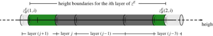
Re-gridding of profile data are done with conservation of mass in mind (or total optical depth, in the case of aerosol data). As an example, assume that a target profile (in partial column units for a concentration profile or optical depth for an aerosol extinction profile) is defined on a vertical height gridzSwith boundarieszSB(the superscript S is used to iden-tify this grid as the source grid). To re-grid the profile to a new grid with layer heights zE and boundaries zEB (E is external), we construct a transformation matrixDthat con-tains the fractions of how each external grid layer is covered by a source grid layer. The coefficients of the transformation matrixDsatisfy 0≤D(i, j )≤1 whereiruns over the
dimen-sion ofzEandj runs over the dimension of the source grid zS. A situation is depicted in Fig. 2, where the external grid is coarser than the source grid (i.e., external layers overlap multiple source layers).
Algorithm. (Layer height weighted re-gridding) Assume the ith coarse grid layer overlaps with the jth source grid
layer. Then the element in theith row ofDcorresponding to thejth source layer is an interpolation factor:
D(i, j )=min z S
B(2, j ),zEB(2, i)−max zSB(1, j ),zEB(1, i)
zSB(2, j )−zSB(1, j ) .
If there is no overlap betweenith external layer andjth
source layer, the corresponding element inD(i, j )equals 0.
For the situation in Fig. 2, the ith row will take the
height boundaries for theith layer ofzE
layer (j+1) layerj layer (j−1) layer (j−3)
zE B(2,i) zE
B(1,i)
height
Figure 2.Interpolation factors for grid layers: green source grid layers are only partially overlapped by theith destination layer.
.5
tM
1 t
M
2 t
M
3 t
M
4 t
M 5
· · · timet tN
1 t
N
2 t
N
3 t
N
4 t
N 5
Figure 3. Temporal co-location of MACC (model, black) and NORS (measurement, green) data.
lower/upper boundary of theith external layer):
D(i, . . .)=(0. . .0
(j−3)
0.42 1 1 1
(j+1)
0.87 0. . .0).
The dark gray layers in Fig. 2 have integer coefficients in Das they are completely covered by theith row ofzEB.
The sum of all rows in the transformation matrix is a vector with the dimension of the source grid that contains a coeffi-cient of 1 for every source layer that is completely covered by an external layer. The re-gridded profile is obtained from matrix multiplication: OR3=D·O3. A final step in the re-gridding process is to set profile values to void (or NaN) for layers of the external grid that are not or only partly covered by the source grid.
3.2 Temporal co-location
Section 2.2 describes the construction of the MACC timely data sequencet1M, t2M, etc. The time between two subsequent
MACC data validity times is constant and denoted by1 >0
(typically1=3 h). Around each MACC timetMthe server
puts a pre-defined time windowδof length 0< δ≤1as
in-dicated in Fig. 3 with a gray rectangle.
A NORS measurement at timetNwill be used to validate
a MACC data instance valid at timetMif|tN−tM|< δ/2.
This choice implies that a single MACC data instance at time tM is validated against several measurements. But
a single measurement will not validate multiple MACC data instances. If a NDACC measurement cannot be related to a MACC time (for instance, in the situation oft4Nin Fig. 3),
the NDACC measurement will not be used in the validation. This type of co-location is used for all NDACC prod-ucts; however, depending on the nature of the species and the availability of measurements, the window δ may differ
from one target species to another (see Table 4). For ex-ample, due to the high diurnal variability of stratospheric NO2, UVVIS.DOAS.ZENITH.NO2 (UVVIS.DOAS stands
for UV–visible (MAX)differential optical absorption spec-troscopy) measurements haveδ=12h.
3.3 Spatial co-location and smoothing
Not all measurement techniques measure the state of the atmosphere directly above the instrument’s location, e.g., FTIR measurements measure direct sunlight, and the probed column of air varies with the local measurement time. A similar situation occurs for UVVIS.DOAS.ZENITH and UVVIS.DOAS.OFFAXIS measurements. The vertical pro-file that is extracted from the MACC model at the site’s lo-cation, should take this off location of the measured air mass into account.
The UVVIS template includes the latitude and longitude coordinate for the probed air mass at each height grid point (the latitude and longitude GEOMS variables). For FTIR measurements, the server uses an off-line routine to calculate the latitude and longitude GEOMS variables when not avail-able in the NDACC file. Depending upon the availability of these variables, the server distinguishes two situations.
3.3.1 Latitude and longitude not available: microwave radiometer and LIDAR
In this case a vertical profile is extracted at the site’s loca-tion by means of a standard bilinear interpolaloca-tion to get from the MACC latitude–longitude grid to a vertical profile at the instrument’s latitude and longitude at all altitudes. The hori-zontally interpolated profile is re-gridded to the measurement vertical grid (i.e., the external grid iszEB=zNBand the source grid iszSB=zMB).
3.3.2 Latitude and longitude available: FTIR and UVVIS.DOAS
If the horizontal coordinates of the probed air mass for each measurement layer are available, the co-located model pro-file is constructed per measurement layer; i.e., the MACC re-gridded profile value for theith measurement grid layerzN equals the value for layeriof the horizontally interpolated
(towards(ϕN(i),λN(i))) and consequently the vertically
re-gridded (towardszN(i)) MACC profile.
The values for the measurement grid that are not (or only partially) covered by the MACC grid are void.
3.3.3 Alignment of re-gridded model data
averag-ing kernel typically acts on VMR profiles. To do this unit conversion, we use temperatureTNand pressurepNprofiles provided along with the measurement data, i.e., the partial column of air for each layer in the measurement grid equals
aN= p
N(i)
RTN(i)1z N.
This implies that the validation is based on the model’s partial column/optical depth profile and that further manipu-lation on both model and measurement data are done using equal conversion factors.
Aerosol optical depth profiles require one further manip-ulation. Typically, the measurement’s optical depth profile is measured at a specific wavelength (sayλN=477 nm) which does not coincide with the wavelength of the model optical depth profile at 532 nm.
Algorithm. (Optical depth wavelength scaling) To con-vert the model optical depth profile to the measurement’s wavelength, we use the Ångström exponent α (Ångström,
1929), calculated from the MACC array of optical depths aergn03 (use the pair of total OD’s at 532 nm and at the wave-length closest to the measurementλN=477 nm, in this case 469 nm):
α= −
lnOD469
OD532 ln
469 532
.
Under the assumption that the Ångström coefficient is height independent and the measurement’s wavelength λN falls within the validity range of the above estimate for α, the re-gridded model optical depth profile is then scaled with the factor
λN 532
−α
.
3.4 Application of the measurement’s averaging kernel In the following, it is understood that the re-gridded model profile, e.g., OM3,R, has been converted to the units of the measurement’s averaging kernel. Smoothing of model profile data ensures that the model profile and measurement profile coincide on height levels outside the measurement’s sensi-tivity range (see also below); i.e., there can be no biases be-tween model and measurement outside the sensitivity range. Furthermore, according to the GEOMS template files (FTIR; UVVIS; see Retscher et al., 2011), the reported measurement uncertainties do not include the smoothing uncertainty which makes the smoothing of model data mandatory in order to have a complete uncertainty budget for the validation statis-tics. Examples of typical AVKs for each measurement tech-nique can be found in the NORS documentation (De Mazière et al., 2013; Richter et al., 2013).
Algorithm. (Smoothing of model data) The smoothed model profile is obtained by the standard smoothing formula
on the re-gridded model profileOM3,R (see Rodgers, 2000, matrix multiplication is used):
OM3,S=ON3,ap+AN·OM3,R−ON3,ap,
where the measurements a priori profileON3,apis used and where the (possibly) void (NaN) re-gridded model profile values are well taken care of. By substituting a zero for these void layers in the difference profileOM3,R−ON3,apand as a fi-nal step, after applying the above smoothing formula, the values in the resulting smoothed model profileOM3,S corre-sponding to the initial void layers of the re-gridded profile are replaced by NaN. In this way, the AVK is applied to the model target profile, even if the model does not provide data on the entire AVK grid. The above method ensures that these outside layers do not contribute in the smoothing operation. Figures 4 and 5 show an example of the above-described re-gridding and smoothing algorithms applied to a stratospheric O3FTIR profile measurement.
In some cases, the measurement data only provide a re-trieved total column (e.g., the UVVIS.DOAS.ZENITH mea-surements). In that case the above formula is adapted such that the column averaging kernel is used. In this caseANis a transformation (with the shape of a vector) acting on pro-files of partial columns, and the result is a scalar total column value:
OM,S,tc
3 =
X
layers
O3N,ap+AN·O3M,R−ON3,ap,
The resulting smoothed model total column/optical depth is void if the measurement grid outranges the model grid. The model grid height typically reaches 65 km. For the FTIR, LI-DAR and microwave radiometer (MWR) data, the measure-ments are reported on grids up to 100 km.
4 Representation of validation results
In order to get statistics on the validation results (see Huijnen and Eskes, 2012), all individual (per measurement) results are brought to a chosen fixed vertical grid. Such a common grid can be a single layer grid to get a partial column or a true vertical grid to calculate a mean (difference) profile. Another possibility implemented by the server, is the re-gridding to-wards a subgrid of the measurement grid where each partial column overlaps layers whose cumulative sum of the degrees of freedom (the diagonal elements of the AVK) is approxi-mately one.
0 5 10 15 20 25
partial column [DU]
0 10 20 30 40 50 60
Height [km]
NORS profile NORS apriori profile MACC original profile MACC smoothed profile MACC regridded (no smoothing)
0 2 4 6 8 10
layer thickness [km]
0 10 20 30 40 50 60
FTIR grid thickness MACC grid thickness
FTIR.O3 JUNGFRAUJOCH: profiles for measurement 2013 Sep 03 07:00:58
Figure 4.Example of a model O3partial column profile (dashed blue) and FTIR measured profile (black). The model profile is first re-gridded to the measurement grid (blue) and smoothed (red) at Jungfraujoch. The lower two horizontal lines show the lowest layer height of the model (lowest) and site (highest). Because a partial column profile depends linearly on the layer thickness of the grid, the right plot shows the layer thickness profile for model and mea-surement grids. Above 40 km the meamea-surement (black), a priori (gray) and smoothed model (red) profiles coincide because the sen-sitivity of the measurement decreases (see Fig. 5).
is done with the algorithm described earlier (i.e., applied to profile data of partial columns/optical depths).
4.1 Uncertainty propagation
NDACC uncertainties can be reported as standard deviation valuesσ, or covariancesS. Uncertainty propagation requires
the knowledge of covariance matrices. If either the system-atic or random uncertainty matrix contains fill values, the ma-trix is filled with NaNs. NaN uncertainties are not shown in the reports.
The measurement uncertainty covariance matrixSN (ran-dom or systematic) is propagated to this chosen represen-tation grid using the transformation matrix Ddescribed in Sect. 3.1 withzNB as source grid and the representation grid as external grid (matrix multiplication):
SE=D·SN·DT.
The covariance matrices in the formula above are in partial column units (e.g., mol m−2). To convert a covariance matrix
0.05 0.00 0.05 0.10 0.15 0.20
10 20 30 40 50 60
Height [km]
FTIR.O3 JUNGFRAUJOCH AVK (rel to apriori) DOF=4.63
Figure 5.Example of a O3FTIR measurement averaging kernel. The plot shows the rows of the AVK matrix, color coded according to the height that corresponds to each row. The matrix elements of an AVK are without unit (the depicted AVK acts on O3profiles rel-ative to the a priori profile). The black dashed line is the sensitivity (the sum of each row): for rows with zero sensitivity the smoothing formula returns the a priori.
in VMR unit to partial column units, the partial column pro-file of airaNis used: the(i, j )th component of the covariance
in VMR units is multiplied with
aN(i)aN(j ).
To transform a covariance matrix from optical thickness units towards optical depth, the same formula is used where aNis replaced by the vector of layer thickness1zN. 4.2 Sensitivity and partial columns
4.3 Time averaging of column data
For long time periods, it is required to average data in time to improve the readability or visibility of the validation statis-tics. For example, assume that the monthly mean of a time series of O3 partial columns is calculated. Due to the
na-ture of systematic and random uncertainties (see Taylor, 1997; JCGM/WG2, 2008), the random uncertaintyσrof the
monthly mean decreases at rate 1/√n, withnthe sample size
(iruns over all measurements in a month):
σ =
v u u t 1
n2
n
X
i=1 σir2.
This differs from the systematic uncertainty on the monthly mean:
σ =1
n
n
X
i=1 σis.
5 Conclusions
This paper documents in detail generic tools for compari-son between data sets related to atmospheric composition, focusing on ground-based remote-sensing data vs. gridded model data. Although comparisons between data sets from two different sources have been performed for many years in the atmospheric scientific community and the basic
con-cepts of co-location and comparisons are known, this is the first time that generic tools have been developed, fully docu-mented and impledocu-mented successfully. It is also the first time that the effective location of the remotely sensed air masses is taken into account for UVVIS and FTIR measurements, at least in an approximate way. Differences in vertical reso-lution of the data are also accounted for. The tools comply with the QA4EO guidelines (see QA4EO, 2010).
The automatic application of the tools requires that the ref-erence data formats comply with the GEOMS generic guide-lines and specific templates per data type. During the devel-opment of the tools, it appeared that some GEOMS guide-lines needed more precise specifications. Also, many incon-sistencies in the data files have shown up and were corrected. The addition of a new data type to the set already cov-ered, is an easy task, because the tools consist of a succes-sion of basic algorithms, of which many are identical for dif-ferent data types. The tools can also be extended easily to comparisons between the ground-based remote-sensing data and satellite data (instead of gridded model data), by adding different co-location algorithms. Such algorithms have been developed previously in the context of the Generic Environ-ment for Calibration/Validation Analysis (the GECA project, funded by ESA) and will be integrated in the toolset in the near future.
Appendix A
Table A1.List of GEOMS variable names, notations and corresponding GEOMS templates.
GEOMS template version GEOMS name Notation
FTIR-002 *.MIXING.RATIO.VOLUME_ABSORPTION.SOLAR O3,CO,CH4,. . .
*.MIXING.RATIO.VOLUME_ABSORPTION.SOLAR_UNCERTAINTY.RANDOM.COVARIANCE Sr
*.MIXING.RATIO.VOLUME_ABSORPTION.SOLAR_UNCERTAINTY.SYSTEMATIC.COVARIANCE Ss
*.MIXING.RATIO.VOLUME_ABSORPTION.SOLAR_APRIORI Oap3, . . .
*.MIXING.RATIO.VOLUME_ABSORPTION.SOLAR_AVK A
MWR-003 O3.MIXING.RATIO.VOLUME_EMISSION O3
O3.MIXING.RATIO.VOLUME_EMISSION_UNCERTAINTY.RANDOM.STANDARD σr
O3.MIXING.RATIO.VOLUME_EMISSION_UNCERTAINTY.SYSTEMATIC.STANDARD σr
O3.MIXING.RATIO.VOLUME_EMISSION_APRIORI Oap3
O3.MIXING.RATIO.VOLUME_EMISSION_AVK A
LIDAR-003 O3.NUMBER.DENSITY_ABSORPTION.DIFFERENTIAL O3
O3.NUMBER.DENSITY_ABSORPTION.DIFFERENTIAL_UNCERTAINTY.ORIGINATOR σr
UVVIS.DOAS.ZENITH-006 *.COLUMN.STRATOSPHERIC_SCATTER.SOLAR.ZENITH Otc
3, NOtc2
*.COLUMN.STRATOSPHERIC_SCATTER.SOLAR.ZENITH_UNCERTAINTY.RANDOM.STANDARD σr *.COLUMN.STRATOSPHERIC_SCATTER.SOLAR.ZENITH_UNCERTAINTY.SYSTEMATIC.STANDARD σs
*.MIXING.RATIO.VOLUME_SCATTER.SOLAR.ZENITH_APRIORI Oap3,. . .
*.COLUMN.STRATOSPHERIC_SCATTER.SOLAR.ZENITH_AVK A
UVVIS.DOAS.OFFAXIS-006 *.MIXING.RATIO.VOLUME_SCATTER.SOLAR.OFFAXIS NO2,HCHO
*.MIXING.RATIO.VOLUME_SCATTER.SOLAR.OFFAXIS_UNCERTAINTY.RANDOM.COVARIANCE Sr
*.MIXING.RATIO.VOLUME_SCATTER.SOLAR.OFFAXIS_UNCERTAINTY.SYSTEMATIC.COVARIANCE Ss
*.MIXING.RATIO.VOLUME_SCATTER.SOLAR.OFFAXIS_APRIORI NOap2,. . .
*.MIXING.RATIO.VOLUME_SCATTER.SOLAR.OFFAXIS_AVK A
AEROSOL.EXTINCTION.COEFFICIENT_SCATTER.SOLAR.OFFAXIS τ
WAVELENGTH λ
AEROSOL.EXTINCTION.COEFFICIENT_SCATTER.SOLAR.OFFAXIS_UNCERTAINTY.RANDOM.COVARIANCE Sr
AEROSOL.EXTINCTION.COEFFICIENT_SCATTER.SOLAR.OFFAXIS_UNCERTAINTY.SYSTEMATIC.COVARIANCE Ss
AEROSOL.EXTINCTION.COEFFICIENT_SCATTER.SOLAR.OFFAXIS_APRIORI τap
Code availability
The code used by the validation server is built on the ex-isting GECA Toolset (Generic Environment for Calibration and Validation Activities), developed within the ESA GECA project. It is foreseen that the GECA Toolset will become publicly available as a separate component in BEAT (Basic Envisat Atmospheric Toolbox) (http://www.stcorp.nl/beat/, an ESA funded project). Until then, the GECA code is avail-able upon request to S. Niemeijer.
Acknowledgements. This work was developed under a EU FP7 project, NORS, under grant agreement no. 284421. The NORS project relies on the data publicly available in NDACC (http://www.ndacc.org). The data providers for FTIR, MWR, LIDAR and UVVIS measurements in the NDACC database are acknowledged. We would like to thank the anonymous referees for their constructive comments.
Edited by: A. B. Guenther
References
Andrews, D.: An Introduction to Atmospheric Physics, Cambridge University Press, Cambridge, 2010.
Ångström, A.: On the atmospheric transmission of sun radiation and on dust in the air, Geogr. Ann. A, 11, 156–166, 1929.
De Mazière, M., Richter, A., Pastel, M., Hendrick, F., Lange-rock, B., and Hocke, K.: NORS Data User Guide, available at: http://nors.aeronomie.be/projectdir/PDF/NORS_D4.2_DUG. pdf (last access: 28 September 2014), 2013.
Huijnen, V. and Eskes, H.: Skill scores and evaluation methodology for the MACC II project. MACC-II VAL D_85.2, avail-able at: http://www.gmes-atmosphere.eu/documents/maccii/ deliverables/val/ (last access: 28 September 2014), 2012.
JCGM/WG2: Evaluation of Measurement Data – Guide to the Expression of Uncertainty in Measurement, Working Group 2 of the Joint Committee for Guides in Metrology, available at: http://www.bipm.org/utils/common/documents/jcgm/JCGM_ 100_2008_E.pdf (last access: 28 September 2014), 2008. Lambert, J.-C.: Validation protocol, available at: http://www.
gmes-atmosphere.eu/documents/deliverables/man (last access: 28 September 2014), 2010.
NIMA: NIMA Technical Report TR8350.2, Department of De-fense World Geodetic System 1984, Its Definition and Rela-tionships With Local Geodetic Systems, Geodesy and Geo-physics Department, National Imagery and Mapping Agency, 3rd Edn., available at: http://earth-info.nga.mil/GandG/publications/ tr8350.2/wgs84fin.pdf (last access: 28 September 2014), 1984. QA4EO: A Quality Assurance Framework for Earth
Observa-tion: Principles, available at: http://qa4eo.org/docs/QA4EO_ Principles_v4.0.pdf (last access: 28 September 2014), 2010. Retscher, C., De Mazière, M., Meijer, Y., Vik, A., Boyd, I.,
Niemei-jer, S., Koopman, R., and Bojkov, B.: The Generic Earth Ob-servation Metadata Standard (GEOMS), available at: http:// avdc.gsfc.nasa.gov/index.php?site=1178067684 (last access: 28 September 2014), 2011.
Richter, A., Godin, S., Gomez, L., Hendrick, F., Hocke, K., Lange-rock, B., van Roozendael, M., and Wagner, T.: NORS Spatial Representativeness of NORS observations, available at: http:// nors.aeronomie.be/projectdir/PDF/D4.4_NORS_SR.pdf (last ac-cess: 28 September 2014), 2013.
Rodgers, C. D.: Inverse Methods for Atmospheric Sounding: The-ory and Practice (Series on Atmospheric Oceanic and Plane-tary Physics), World Scientific Publishing Company, Singapore, 2000.