UNIVERSIDADE NOVA DE LISBOA
Faculdade de Ciências e Tecnologia
Depº de Ciências e Engenharia do Ambiente
Monitoring Chlorophyll-
a
with remote sensing
techniques in the Tagus Estuary
Akli Ait Benali
Dissertação apresentada na Faculdade de Ciências e
Tecnologia da Universidade Nova de Lisboa para obtenção
do grau de Mestre em Gestão e Sistemas Ambientais
Orientador :
Doutora Maria Júlia Fonseca Seixas
Co-Orientador : Doutor João Gomes Ferreira
Acknowledgments
This work has been one big and rocky road with lots of signs and complications. Many have a been part of it, and I dedicate my work to you all. First, my family, the ones who have suffered the most from the lack of patience, humour and lots of nerves. This road has been possible because of you and remember, every step was taken aiming at making you proud. Thank you. Second, to my girlfriend Liandra. I know that this thesis as been my primary lover for the last year, but you were always a fantastic “part time” lover ;) Thanks for the patience and confort you have provided, and forgive me for the lack of the same. I love you with all my heart.
I would like to thank my scientific advisors, Drª Júlia Seixas and Drº João Gomes Ferreira, for the support, advises and expert knowledge. Also, thanks to Ricardo Pacheco and Bruno Urmal for the technical expertises in informatics, namely in the help provided using the Linux environment. It was a smooth shock thanks to you both. Special thanks for the NASA Ocean Color Group which provided extremely valuable technical assistance in ocean color issues and SeaDas handling. You were fantastic and without you this work would have been far more difficult and probably not ready on time. Many thanks to Vânia Bento for the help with the EcoWin2000 initial model handling.
Thanks to Nuno Grosso, Joana Monjardino and Mario Sanches for the last call urgent help. Particularly the former, for the brief and helpful insights on remote sensing of atmosphere. Special thanks to João Pedro Nunes and Nuno Carvalhais for the interesting and very helpful scientific coffee breaks. I didn’t know that coffees had so much to teach, thank you very much. Particularly Carvalhais, thanks for some of your MatLab functions and knowledge provided during the CARBERIAN project. It made a huge difference.
Resumo
Os estuários são ecossistemas de transição com elevada variabilidade espacial e temporal, sujeitos a elevadas pressões antropogénicas. Actualmente é um desafio monitorizar estes sistemas de uma forma robusta, frequente, sistemática e com precisão adequada. Com a implementação da Directiva Quadro Agua, os estados membros da UE são obrigados a monitorizar regularmente os parâmetros biológicos e físicos mais relevantes. A informação sobre um estuário é adquirida recorrendo a dados de campo, implementação de modelos e/ou através de detecção remota.
Avaliou-se a aplicabilidade e precisão de produtos de clorofila-a do sensor MODIS no estuário do Tejo comparando-os (2000-2002) com estimativas de um modelo ecológico, o EcoWin2000, previamente calibrado (1998 e 1999) e validado (2000). Propõe-se um quadro conceptual e metodológico para futura monitorização do estuário usando detecção remota.
Numa primeira etapa, os algoritmos típicos para águas tipo 1 foram avaliados e os algoritmos tipo 2 foram calibrados em 2000. Os algoritmos GSM e Clark tiveram as melhores performances, com erros na ordem dos 1.1 g chl-a l-1 (ou 20%) e correlações de 0.4-0.5. Na calibração o rácio R678/R551 apresentou uma correlação razoável (r = 0.83) e com baixos
erros (~1 g chl-a l-1). A sua avaliação em 2002 evidenciou correlações baixas e negativas
com erros na ordem dos 2 g chl-a l-1. Em concordância com a avaliação preliminar, em 2002, o algoritmo GSM apresentou a melhor correlação (r~0.50) com erros á volta de 0.8 g chl-a l
-1. A fiabilidade da aplicação dos produtos de detecção remota é superior na primavera e verão,
e espacialmente, nas secções médias mais largas.
Abstract
Estuaries are transitional ecosystems with high temporal and spatial variability and suffer high anthropogenic pressures. At the present there is a major challenge to monitor these systems in a robust, frequent, systematic and accurate fashion. With the implementation of the Water Framework Directive (WFD), the EU Member States must monitor regularly the most relevant physical and biological parameters. Estuarine information is attained using in-situ samples, model analysis and/or remote sensing data.
This work assessed the applicability and accuracy of chlorophyll-a products from the MODIS sensor in the Tagus estuary, comparing them (2000-2002) with simulations of an ecological model, the EcoWin2000. The latter was previously calibrated (1998 & 1999) and validated (2000). It is proposed a conceptual and methodological framework for future monitoring of the estuary using remote sensing data.
In a first stage, in the year 2000, typical Case 1 algorithms were pre-assessed and Case 2 algorithms were regionally calibrated. The GSM and Clark algorithms had the best performances, with errors of approximately of 1.1 g chl-a l-1 (or 20%) and correlations
ranging 0.4-0.5. During calibration, the ratio R678/R551 had a good correlation (r = 0.83) and
low errors (~1 g chl-a l-1). Its evaluation in 2002, showed low and sometimes negative correlations, with errors of about 2 g chl-a l-1. In agreement with the preliminary assessment, in 2002, the GSM algorithm had the best correlation (r~0.50) and errors of approximately 0.8 g chl-a l-1. The reliability of remote sensing is higher in the Spring and Summer, and spatially, in the wider mid estuary sections.
Acronyms
AOP : Apparent Optical Property
B2k : BarcaWin2000 ®
Chl-a : Clorophyll-a concentration CDOM : Colored Dissolved Organic Matter CO2 : Carbon dioxide
CSZS : Coastal Zone Color Scanner DIN : Dissolved Inorganic Nitrogen
E2K : EcoWin2000 ®
EEA : European Environmental Agency
EU : European Union
FLH : Fluorescence Line Height
FW : Fresh Weight
GPP : Gross primary production
GSM : Garver-Siegel-Maritorena Algorithm
INAG : Instituto Nacional da Agua (Portuguese National Water Institute) IOCCG : International Ocean-Color Coordinating Group
IOP : Inherent Optical Property
L1B : Level 1B
L2 : Level 2 (products)
LAADS : Level 1 and Atmosphere Archive and Distribution System MAE : Mean Absolute Error (%)
MODIS : MODerate resolution Imaging Spectroradiometer MERIS : European MEdium Resolution Imaging Spectrometer
N : Nitrogen
NASA : National Aeronautics and Space Administration NIR : Near Infrared
nLw : Normalized Water Leaving Radiance NPP : Net Primary Production
OOP : Object Oriented Programming SeaDas : SeaWifs Data Analysis System SPM : Suspended Particulate Matter STD : Standard Deviation
P : Phosphorous
PAR : Photosynthetically Available Radiation
PC : Personal Computer
r : Correlation coefficient Rrs : Remote sensing reflectance RMSE : Root Mean Square Error
SEAWIFS : SEA-viewing WIde Field of view Sensor
Si : Silicate
USEPA : United States Environmental Protection Agency VBA : Visual Basic for Applications
VNIR : Visible and Near Infrared WFD : Water Framework Directive WWTP : WasteWater Treatment Plants Zeuph : Euphotic zone depth
Index
1. Introduction ... 11
2. Remote sensing of estuarine chl-a: State of the Art... 19
2.1 - Estuarine Dynamics ... 19
2.1.1 - Light ... 20
2.1.1.1 - Incident Surface Radiation and Sub Surface Attenuation ... 20
2.1.1.2 - Photosynthetic Response ... 23
2.1.2 - Nutrients ... 24
2.1.3 - Hydrodynamics ... 26
2.2 - Remote Sensing Techniques... 29
2.2.1 - Remote Sensing of Ocean Colour... 29
2.2.2 - Remote sensing of Case 2 waters... 32
2.2.3 - Remote Sensing Sensors and Algorithms for chlorophyll monitoring ... 36
3. Methodology... 40
3.1 - Study area: The Tagus Estuary... 40
3.1.1 - General Description... 40
3.1.2 - Hydrodynamics ... 42
3.1.3 - Light and Suspended Particulate Matter... 44
3.1.4 - Nutrients ... 45
3.1.5 - Phytoplankton ... 47
3.2 – Procedures of Model Calibration and Assessment (adapted from Janssen & Heuberger, 1995) ... 49
3.3 - Ecological Model Calibration... 53
3.3.1 - General Considerations ... 53
3.3.2 - EcoWin2000 Description (adapted from Ferreira, 1995)... 56
3.3.3 - Spatial Domain... 58
3.4 - EcoWin2000 Object Calibration... 61
3.4.1 - Sensitivity Analysis... 61
3.4.2 - Light ... 63
3.4.3 - River Flow ... 64
3.4.4 - Hydrodynamics ... 65
3.4.5 - Dissolved Substances ... 68
3.4.6 - Suspended Particulate Matter ... 73
3.4.7 - Zooplankton ... 76
3.4.8 - Phytoplankton ... 77
3.5 - Remote Sensing Data Processing ... 82
3.5.1 - Atmospheric Correction ... 83
3.5.2 - Quality Control ... 86
3.5.3 - Data Temporal and Spatial Compositing ... 88
3.6 - Remote Sensing Regional Calibration ... 91
4. Results and Discussion... 98
4.1 - Ecological Model Validation... 98
4.2 - Remote Sensing Preliminary Assessment ... 102
4.2.1 - Performance of Case 1 Algorithms (2000)... 102
4.2.2 - Performance of Case 2 Algorithms (2000)... 109
4.3 - Case 1 and Case 2 Algorithms: Independent Assessment (2002) ... 115
5. Limitations and Future Work ... 121
6. Conclusions ... 126
Index of Figures
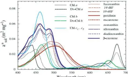
Figure 1 - In vivo weight-specific absorption spectra of the main pigments, a*sol,i( ) in m2
mg-1 (taken from Bricaud et al., 2004)... 33
Figure 2 - Average CDOM (filled) and chlorophyll-specific (clear) absorption spectra for Narragansett Bay (taken from Keith et al., 2002)... 34
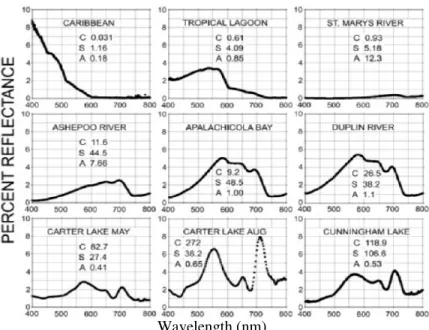
Figure 3 - Water reflectance spectra measured at various coastal, estuarine, and inland locations representing a broad range of optically active constituents. ... 34
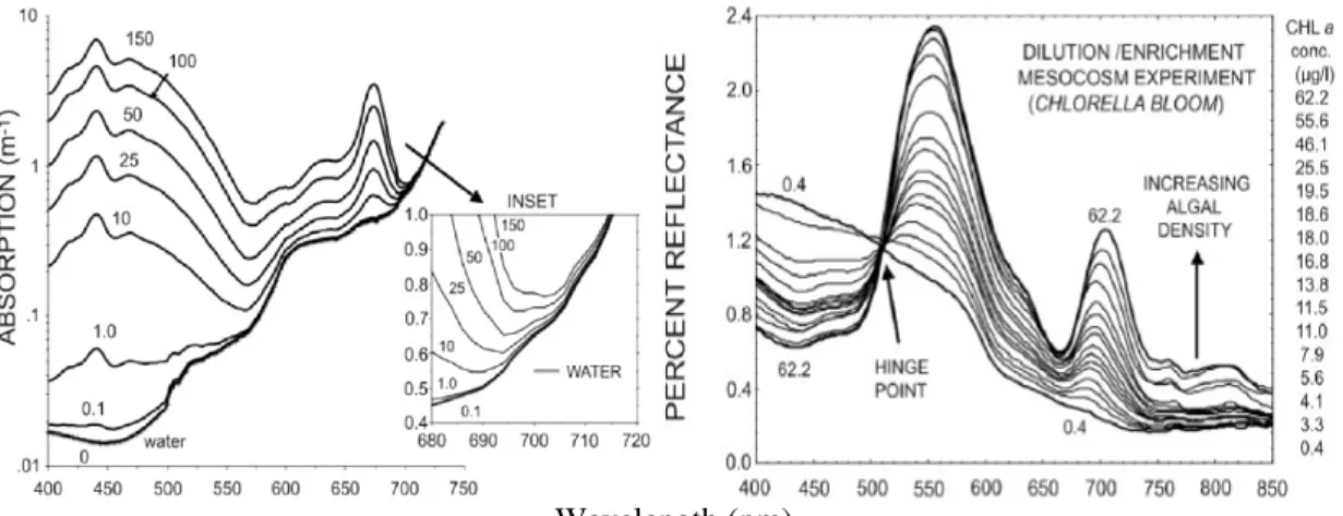
Figure 4 -On the left: Combined absorption coefficients for water and phytoplankton pigment at different concentrations (Bidigare et al., 1990 & Smith and Baker, 1991 in Schalles, 2006). On the right: Graded series of reflectance spectra for different chl a levels for a dilution/enrichment scheme experiment (taken from Schalles et al., 1997 in Schalles, 2006) 35 Figure 5 - Bathymetry, Intertidal Areas and Wetlands in Tagus estuary... 40
Figure 6 - Tagus river watershed land use Corine2000 ... 41
Figure 7 - Model boxes and station sampling locations... 59
Figure 8 - Daily average radiation: observed vs. simulated ... 63
Figure 9 - Monthly averaged daily Tagus Flow (m3s-1) for 1998 and 1999... 65
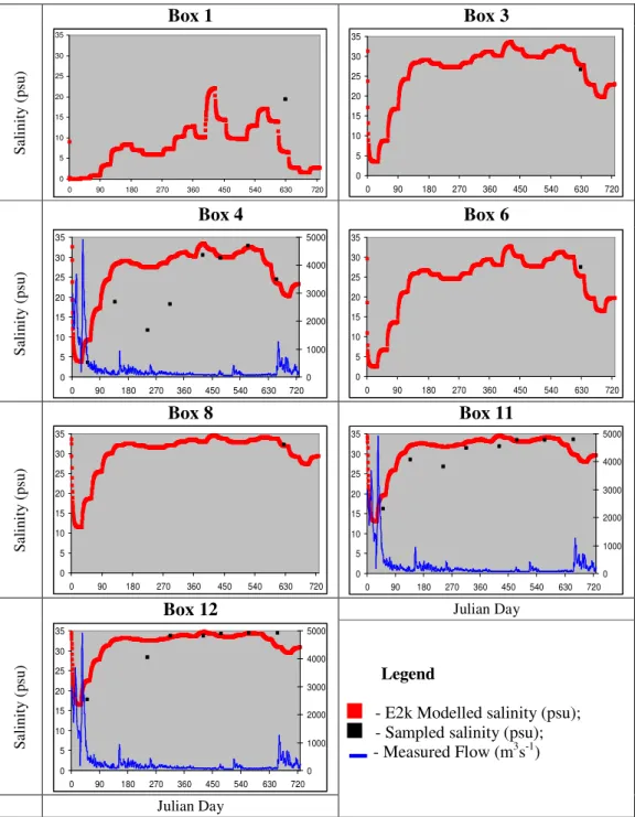
Figure 10 - Salinity time series box by box: sampled vs. modelled ... 68
Figure 11 - Nitrogen to Phosphate (N:P) and Silicate to Phosphate ratio (Si:P)... 69
Figure 12 - Nitrogen to Silicate ratio (N:Si) in atoms... 70
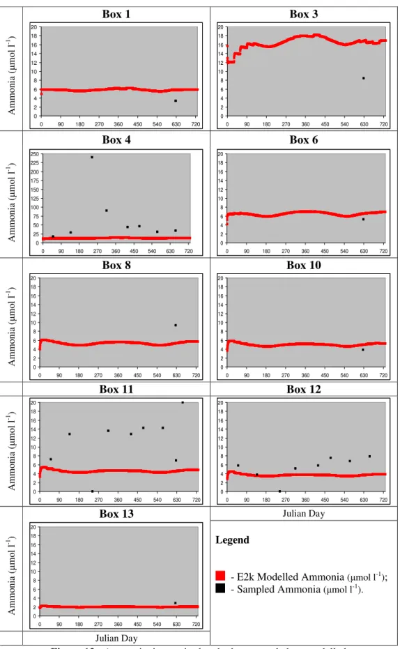
Figure 13 - Ammonia time series box by box: sampled vs. modelled... 71
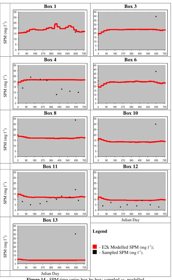
Figure 14 - SPM time series box by box: sampled vs. modelled... 74
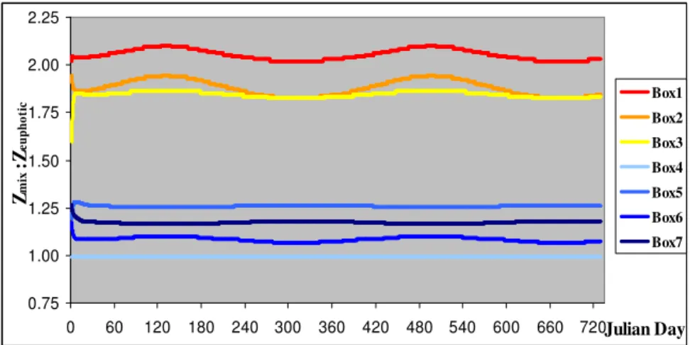
Figure 15 - Modelled Zmix:Zeuphotic in the upper and mid estuary model boxes ... 76
Figure 16 - Cost Function 3D plot: Parameter combination (Pmax and Iopt) ... 79
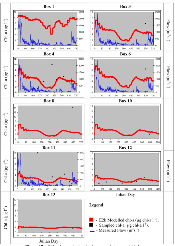
Figure 17 - Chl-a time series box by box: sampled vs. modelled... 80
Figure 18 - Atmospheric correction procedure : Time series Box 10 - 2000... 84
Figure 19 - Atmospheric correction procedure : Time series Box 8 - 2000... 85
Figure 20 - Correlation and RMSE distribution, per box, using different atmospheric procedures : 2000... 85
Figure 21 -Quality Flags and Restrictions : Time series for Box 9 – 2000... 87
Figure 22 - Geometry (solar and sensor zenith angle) vs. Error : 2000 ... 88
Figure 23 - Number of files in a composite vs. [chl-a] : 2000... 89
Figure 24 -Spatial histograms : Box 8 – 2000 ... 90
Figure 25 - OC3 regional calibration (2000)... 92
Figure 26 - Spectral Signatures for all boxes per season : 2000... 93
Figure 27 - Spectral Signatures over time for box 7... 94
Figure 28 -Calibration plot using the ratio R678/(R551+R748) : 2000 ... 97
Figure 29 - Main methodological steps and connections... 97
Figure 30 - Pairwise Scatter plot: sampled vs. simulated ... 98
Figure 31 - E2k chl-a validation, time series box by box: sampled vs. modelled ... 99
Figure 32 - Case 1 algorithms performance: time series for box 7 - 2000... 103
Figure 33 - Case 1 algorithms performance: time series for box 11 - 2000... 103
Figure 34 - Case 1 algorithms performance per box : 2000... 104
Figure 35 - Case 1 algorithms performance per box : 2000... 105
Figure 36 - Chl-a concentration vs. Depth: GSM algorithm 2000 ... 106
Figure 37 - Case 1 Algorithms RMSE distribution: box 9 2000 ... 107
Figure 38 - Standard Processing options – Performance per box : 2000... 109
Figure 39 - OC3 fitted vs. original OC3 : box 10 – 2000... 110
Figure 40 - Tuned OC3 performance : 2000 ... 110
Figure 41 - Case 2 algorithms performance per box : 2000... 111
Figure 42 - Case 2 algorithms : time series for box 7 - 2000 ... 112
Figure 44 - Case 1 algorithms : time series for box 8 - 2002 ... 115
Figure 45 - Case 1 algorithms performance per box : 2002... 116
Figure 46 - Case 1 algorithms Pairwise and MAE(%) distribution for box 10 (2002)... 116
Figure 47 - GSM chl-a spatial 16day distribution: 113-128 (2002) ... 117
Figure 48 - Case 2 algorithms : time series for box - 2002 ... 118
Figure 49 - Case 2 algorithms performance per box : 2002... 119
Figure 50 - Spectral Signatures for all boxes per season : 2002... 120
Figure 51 - Pairwise scatter plot: hourly radiation values (2002) ... 142
Figure 52 - Pairwise scatter plot: hourly radiation values (2003) ... 143
Figure 53 - Daily average radiation values distribution (Monte da Caparica) ... 143
Figure 54 - Pairwise scatter plot : Daily flow m3s-1 (2002 and 2003) ... 144
Figure 55 - Pairwise salinity comparison: measured vs. modelled... 145
Figure 56 - Reference time series box by box: Sampled vs. modelled ... 146
Figure 57 - SPM Calibration using auxiliary data, box by box: sampled vs. modeled... 148
Figure 58 - Pollution Sources in the Tagus watershed... 152
Figure 59 - Nitrate Calibration box by box: sampled vs. modelled... 153
Figure 60 - Phosphate Calibration box by box: sampled vs. sampled ... 154
Figure 61 - Silicate Calibration box by box: sampled vs. modelled ... 155
Figure 62 - MAE (%) 3D plot: Parameter combination (Pmax and Iopt)... 156
Figure 63 - Pearson correlation coefficient 3D plot: Parameter combination (Pmax & Iopt) .. 156
Figure 64 - RMSE 3D plot: Parameter combination (Pmax & Iopt)... 157
Figure 65 - Nitrate Validation box by box: sampled vs. modelled ... 160
Figure 66 - Ammonia Validation box by box: sampled vs. modelled ... 161
Figure 67 - SPM Validation box by box: sampled vs. modelled... 162
Figure 68 - Atmospheric correction procedure : Time series Box 7 - 2000... 163
Figure 69 - Atmospheric correction procedure : Time series Box 9 - 2000... 163
Figure 70 - Atmospheric correction procedure : Time series Box 7 - 2001... 164
Figure 71 - RMSE distribution over the model boxes : 2000... 164
Figure 72 - Correlation distribution over the model boxes : 2001 ... 164
Figure 73 - Quality Control Options : Time series Box 7 - 2000 ... 165
Figure 74 - Quality Control Options : Time series Box 11 - 2000 ... 165
Figure 75 - Quality Control Options : Time series Box 08 - 2001 ... 166
Figure 76 - Quality Control Options : Time series Box 13 - 2001 ... 166
Figure 77 - Geometry (solar and sensor zenith angle) vs. RMSE : 2001... 166
Figure 78 - Daily chl-a images before (left) and after (right) straylight correction... 167
Figure 79 - Outlier and Tidal Height impact on 16day composites : 2000... 168
Figure 80 - Tidal state impact on 16day composites : 2000... 169
Figure 81 - Spatial histograms : Box 10 – 2000 ... 170
Figure 82 - Spatial histograms : Box 12 – 2000 ... 170
Figure 83 - Spatial histograms : Box 6 – 2001 ... 171
Figure 84 - Spatial histograms : Box 11 – 2001 ... 171
Figure 85 - Spectral Signatures for all boxes per compositing period : 2000 ... 172
Figure 86 - Spectral Signatures all boxes per compositing period:2001 ... 173
Figure 87 - Calibration plot using the ratio R678/ R551 : 2000... 174
Figure 88 - Calibration plot using the Fluorescence Line Height : 2000... 174
Figure 89 - Predictions vs. Observations using the ratio R678/ R551(blue); Chl-a temporal distribution (2000) ... 174
Figure 90 - Existing Algorithms Pre-Assessment : Time Series 2000 ... 176
Figure 91 - Case 1 Algorithms RMSE distribution: box 13 2000 ... 176
Figure 92 - Existing Algorithms Pre-Assessment : Time Series 2001 ... 177
Figure 93 - Case 1 Algorithms RMSE distribution: box 8 2001 ... 177
Figure 95 - Case 1 algorithms performance per box : 2001... 178
Figure 96 - Chl-a concentration vs. Distance to Ocean: GSM algorithm (2000) ... 178
Figure 97 - Chl-a concentration vs. 16day Flow: Carder algorithm in 2000 for box 9, r=0.63 (on the left) and box 8, r=0.50 (on the right)... 179
Figure 98 - Performance comparison Cor3 and MUMM atmospheric correction procedures, using the OC3 algorithm (2000)... 179
Figure 99 - Comparison of OC3 tuned vs. OC3 original: Time Series 2000... 180
Figure 100 - Tuned OC3 performance : 2001 ... 181
Figure 101 - Time Series of all Case 2 regional algorithms (2000) ... 181
Figure 102 - Case 1 Algorithms Assessment : Time Series 2002 ... 183
Figure 103 - Case 2 Algorithms Assessment : Time Series 2002 ... 184
Figure 104 - Tuned OC3 performance : 2002 ... 184
Figure 105 - Spectral signatures all boxes per compositing period:2002 ... 186
Figure 106 - Spectral signature distribution over time (2002) ... 187
Index of Tables Table 1 - Monitoring Frequencies for possible remote sensing parameters (adapted from Ferreira et al., 2007b)... 15
Table 2 - In-Situ Data Characteristics ... 55
Table 3 - Model Boxes: Description and morphology... 60
Table 4 - Sensitivity Analysis: Forcing Functions and State Variables (in %) ... 61
Table 5 - Sensitivity Analysis: Dissolved Substances Object (in %)... 62
Table 6 - Sensitivity Analysis: Phytoplankton Object (in %)... 62
Table 7 - Statistics of modelled flow values (m3s-1) in the calibration years ... 64
Table 8 - Transport object performance statistics: box by box and ecosystem scale ... 67
Table 9 - Ammonia Calibration: performance statistics box by box and ecosystem scale ... 72
Table 10 - Comparison of simulated nutrients with Gameiro et al. 2007 ... 72
Table 11 - SPM object performance statistics: box by box and ecosystem scale... 75
Table 12 - Comparison of simulated SPM with Gameiro et al. 2007 (adapted) ... 75
Table 13 - Phytoplankton Productivity: Equations (Ferreira et al., 1998) ... 77
Table 14 - Phytoplankton object : equations and processes (Ferreira et al., 1998) ... 78
Table 15 - Phytoplankton object performance statistics: box by box and ecosystem scale.... 79
Table 16 - Atmospheric correction procedures tested... 84
Table 17 - Quality Control flags tested ... 86
Table 18 - Description and performance of regionally calibrated algorithms... 96
Table 19 - Phytoplankton object performance statistics: box by box and ecosystem scale.... 98
Table 20 - Comparison of simulated chl-a with Gameiro et al. 2007 (adapted)... 100
Table 21 - Regression statistics between Monte Caparica and Vila Franca de Xira stations 142 Table 22 - Set of parameters used in the light object calibration... 144
Table 23 - E2k flow simulation performance ... 145
Table 24 - Statistics regarding monthly averaged daily flows (polynomial) ... 145
Table 25 - Parameters achieved in SPM calibration (sampled data) ... 147
Table 26 - Historical and reference studies comparison ... 147
Table 27 - Parameters achieved in SPM calibration (historical and reference data) ... 147
Table 28 - Parameters used in the zooplankton object... 149
Table 29 - Boundary conditions for the Tagus river and ocean – Calibration ... 150
Table 30 - Boundary conditions for the Tagus river and ocean – Calibration ... 151
Table 31 - Boundary description and setting for smaller estuary affluents (Ferreira, personal communication; INAG, 2002 and www.insaar.inag.pt ) ... 151
Table 33 - Phosphate Calibration : performance statistics box by box and ecosystem scale 152
Table 34 - Silicate Calibration : performance statistics box by box and ecosystem scale.... 152
Table 35 - MAE (%): Parameter combination (Pmax & Iopt) ... 157
Table 36 - Pearson Correlation Coefficient : Parameter combination (Pmax & Iopt)... 157
Table 37 - RMSE: Parameter combination (Pmax & Iopt) ... 158
Table 38 - Cost function: Parameter Combination (Pmax & Iopt)... 158
Table 39 - Phytoplankton object performance statistics for Iopt = 300 & Pmax = 0.075 ... 158
Table 40 - Phytoplankton object performance statistics for Iopt = 600 & Pmax = 0.1 ... 158
Table 41 - Case 1 algorithms performance for the year 2000 - MAE (%)... 175
Table 42 - Case 1 algorithms performance 2000 - RMSE ( g chl-al-1) ... 175
Table 43 - Case 1 algorithms performance for the year 2000 - correlation (r) ... 175
Table 44 - Case 1 algorithms performance for the year 2001-MAE (%)... 175
Table 45 - Case 1 algorithms performance for the year 2001 - RMSE ( g chl-a l-1) ... 175
Table 46 - Case 1 algorithms performance for 2001 - correlation (r)... 175
Table 47 - Case 2 algorithms performance for the year 2000 - RMSE ( g chl-a l-1) ... 182
Table 48 - Case 2 algorithms performance for the year 2000 – MAE (%) ... 182
Table 49 - Case 2 algorithms performance for the year 2000 - Correlation... 182
Table 50 - Case 1 algorithms performance for 2002 - MAE (%) ... 185
Table 51 - Case 1 algorithms performance for 2002 - RMSE ( g chl-a l-1)... 185
Table 52 - Case 1 algorithms performance for 2002 - correlation (r)... 185
Table 53 - Case 2 algorithms performance for year 2002 - RMSE ( g chl-a l-1) ... 185
Table 54 - Case 2 algorithms performance for the year 2002 – MAE (%) ... 185
Table 55 - Case 2 algorithms performance for the year 2000 - Correlation... 185
Index of Annexes
Annex I : Forcing Functions Calibration Annex II : SPM and Zooplankton Calibration
Annex III : Boundary Conditions & Dissolved Substances Calibration Annex IV : Phytoplankton Object Calibration
Annex V : Validation of the Dissolved Substances and SPM objects Annex VI : Atmospheric Correction Procedures
Annex VII : Quality Control Masking
Annex VIII : Temporal and Spatial Compositing
Annex IX : Regional Calibration of Case 2 Algorithms
Annex X : Preliminary assessment of Case 1 chl-a algorithms Annex XI : Preliminary assessment of regionally tuned algorithms
1. Introduction
Transitional waters are surface water bodies near river mouths which are partly saline as a result of their proximity to coastal waters and are substantially influenced by freshwater flows (Chen et al., 2004). These systems are important and valuable in terms of biodiversity, ecology, support to human populations and role in the connection between terrestrial and aquatic ecosystems. Furthermore, over 50% of human populations live in coastal zones (e.g. Richardson & Ledrew, 2005). Estuaries, included on this surface water category, are highly productive ecosystems usually enriched with nutrients, in comparison with most offshore waters (e.g. Ketchum, 1967 in Liu, 2005), and have multiple sources of organic carbon to sustain populations of heterotrophs. Colored dissolved matter, suspended sediments and phytoplankton typically have higher concentrations in estuaries, when compared to oceans (e.g. Richardson & Ledrew, 2005). Estuaries are highly sensitive to climate variability, although, their communities are well adapted to temporal variability and spatial gradients such as salinity or temperature (e.g. Gameiro, et al 2007).
In estuaries there are three main types of producers: phytoplankton, benthic algae and vascular plants, which ensure maximum utilization of light and nutrients, mixed by the water movement due to tidal action and freshwater flow (e.g. Trancoso, 2002). Producers are the basis of the trophic chain supporting countless ramifications. In most estuaries, phytoplankton is usually the most relevant contributor to total production (e.g. Day et al., 1989) and, therefore, it is a key component in these systems providing an essential ecological function for all aquatic life (e.g. Lucas et al., 1999a). The consequent intense bacterial activity promotes rapid cycling of nutrients, which along with the hydrodynamic conditions, gives estuaries the unique capacity of self-depurating systems (e.g. Trancoso et al., 2005). The central biological variable for phytoplankton is upper-layer chlorophyll-a concentration (hereafter chl-a), which can be used to estimate phytoplankton standing stocks and productivity throughout the photic zone (e.g. Behrenfeld et al., 2006).
have suggested that phytoplankton can be a solution to reverse the accumulation of anthropogenic carbon dioxide (CO2) in the atmosphere (Richtel, 2007). Everyday more than
100x106 tons of carbon, in the form of CO
2, are fixed into organic material by phytoplankton
and a similar amount of organic carbon is transferred to aquatic ecosystems by sinking and grazing (Behrenfeld et al., 2006). There is still great uncertainty in the scientific community concerning the overall magnitude of global primary production, with estimates varying from 27.1 (Eppley & Peterson, 1979) to 50.2 Gt Cy-1 (Longhurst et al., 1995). Considering only coastal ecosystems’ global production, estimates range between 8.9 and 14.4 Gt Cy-1
(Longhurst et al., 1995). Day et al. (1989) estimated an average phytoplankton production in estuaries of 256 gCm-2 y-1, well above typical values (100 gCm-2 y-1). In temperate estuaries, the typical primary production rates are 160 gCm-2 y-1 and lower values may indicate light limitation (Heip et al., 1995). Estuarine productivity can sometimes be deceiving, where annual phytoplankton production can be less than that of other marine environments (Cloern, 1987). In fact, Borges et al. (2006) stated that estuaries are significant sources of CO2 to the
atmosphere, at an average rate of 49.9 molC m-2 yr-1, corresponding to a scaled emission over Europe, of 67.0 TgC yr-1.
Regular monitoring of surface water status is fundamental to obtain estuarine information and to better understand its dynamics. Monitoring is carried out by assessing a range of quality parameters, which usually varies both, in time and space. Logistical and financial resource limitations are important factors controlling the scope and range of monitoring activities. It is necessary to develop robust and low cost tools, which support monitoring activities, ensuring that objectives are accomplished and enabling optimisation, quality and reliability (Ferreira et al., 2007b).
The Water Framework Directive (WFD), approved by the European Union (E.U.), establishes a set of water quality objectives and the overall goal is to achieve good water status for all E.U. waters by the year 2015. In the scope, application and practical implementation of the Directive, regular monitoring is stated as fundamental and determines water bodies classification and the need for additional measures to achieve its objectives. Member States must establish monitoring plans to regularly assess their aquatic ecosystems ecological status, determining their compliance, and must report to the European Environmental Agency (EEA) every two years (Chen et al., 2004; Ferreira et al., 2007b). According to the WFD, phytoplankton is considered to be a key biological quality element for transitional and coastal waters. The main parameters are composition, abundance and biomass (i.e. chl-a concentration), which also integrate other relevant indicators (Bricker et al., 1999; Bricker et al., 2003; ICES, 2004; Ferreira et al., 2005a & 2007b).
annual monitoring program, the former can reach up to approximately 90% of the total cost due to the higher number of inshore water bodies, number of sampling stations and monitoring frequency (Ferreira et al., 2005b).
To overcome some of the limitations of in-situ sampling, modelling is used to develop hypotheses and understanding the ecosystem’s dynamics, through simulation of the main processes. This is accomplished by using mathematical modelling that typically investigates the influence of each factor and then combines it in an ecosystem approach. Monitoring provides the necessary data to model setup, calibration and validation, while models provide knowledge on systems and processes that may improve the monitoring programme (Ferreira et al., 2005b). Furthermore, it enables the simulation of several scenarios thru testing and prediction (Ferreira et al., 2005b; Neves et al., 2000 in Trancoso et al., 2005), and spatial and temporal filling of information blanks. Therefore, modelling and monitoring are tightly coupled and the former may improve the efficiency by reducing the need for resources whilst achieving the defined objectives (Ferreira et al., 2007). Several studies have been conducted using modelling approaches (e.g. Trancoso et al., 2005; Nobre et al., 2005; Nunes et al., 2003; Ferreira, et al., 2007a) and specifically in the Tagus estuary (e.g. Antunes, 1998; Saraiva, 2001; Trancoso, 2002; Ferreira, 1989; Portela, 1996; Alvera-Azcárate et al., 2003). Data availability is still considered to be the most important factor limiting the development of operational water quality models (James, 2002) while the compilation of a database for comparison purposes and system understanding is mainly being limited by scarce spatial and temporal data (Monbet, 1992). Modelling accuracy is limited by the calibration and validation data and, although a valuable tool, does not provide real system information.
associated continually expandable historical archives, the detection and spatial distribution of changes in water bodies. Remote sensing can also establish information datasets regarding point and diffuse sources of pollution mapping relevant to emission control and support the establishment of river basin management plans. Particularly under the WFD, these benefits have high potential to support the establishment of the monitoring programmes’, and thus, to assist EU states meet their obligation under the very demanding timetable and resource limitation (Chen et al., 2004).
Remote sensing has been widely used in monitoring Case 1 waters, in which the principal component is chl-a usually in low concentrations. There is a growing concern in using remote sensing to monitor optically complex Case 2 waters. By using current advanced satellite sensors, a large number of water quality variables can be monitored on a regular basis, for instance, chl-a, total suspended sediment, type of particulate content, yellow substance or
gelbstoff, turbidity, Secchi disk depth, wave height, colour index and surface water
temperature (e.g. Zhang et al., 2002b; Chen et al., 2004). Proposed parameters and their frequencies for surveillance monitoring according to the WFD are described in Ferreira et al. (2007). Table 1 exhibits only the parameters with potential for direct or indirect remote sensing acquisition.
Table 1 - Monitoring Frequencies for possible remote sensing parameters (adapted from Ferreira et al., 2007b)
Water Bodies Quality Type Parameter Frequency
Biological Phytoplankton Seasonal/
Six Months
Turbidity Seasonal
Open Coastal water
bodies Physico-chemical
Temperature Seasonal
Phytoplankton
(biomass & abundance) Monthly Biological
Phytoplankton species
composition Six Months
Coastal and transitional water bodies
Physico-chemical Temperature Monthly
composition. Suspended particulate matter (SPM) can be estimated thru remote sensing in coastal waters with good accuracy (e.g. Miller and Mckee, 2004; Doxaran et al., 2002a & 2002b; Li et al., 2003; Doerffer and Schiller, 2007; Zawada et al., 2007; Chen et al., 2007; Hu et al., 2004), providing frequent synoptic maps of turbidity. Water surface temperature has been estimated using remote sensing techniques, mainly in deep sea and open coast systems (e.g. Zhang et al., 2002b; Zhang et al., 2004; Chan and Gao, 2005; de Souza et al., 2006; Vander Woude et al., 2006; Barré et al., 2006), and scarcely in transitional inshore systems (e.g. Davies, 2004; Li et al., 2001) The principal aim of surface temperature is to study global scale temperature dynamics, for instance for climate change assessment and research purposes.
The role of remote sensing technology is presently under scrutiny and several conceptual and practical requirements need to be fulfilled, such as an incomplete technical and scientific basis, to optimize the support for regional and global scale water status monitoring (Ferreira et al. 2007b, Chen et al., 2004). Remote sensing provides information mainly on the surface layer and thus, when vertical sampling is necessary it provides valuable but incomplete information. Another limitation is related to operational constraints on systematic remote sensing monitoring. According to some authors, accessibility, poor management, inadequate trained staff and knowledge transfer need to be improved to facilitate further research, training and education in remote sensing practical applications (Rosenqvist et al., 2003; Kalluri et al., 2003 in Chen et al., 2004). The cost of remotely sensed data can also, in some cases, be a major limitation. Low resolution and product accuracy are important issues concerning reliability and practical implementation, especially in inshore systems (e.g. Tzortziou et al., 2007; Chen et al., 2004). There is a trade-off between remote sensing data cost, quality and application coverage. For instance, the MODIS sensor provides traditionally 1km resolution data at no cost, whilst, the MERIS sensor provides 300m resolution data but with use restrictions.
phytoplankton temporal and spatial dynamics in estuaries. For estuarine applications, one of the major challenges is to develop multisource monitoring procedures, associating different sources of information, thus, minimizing their limitations and flaws (Prandle, 2000).
This work assesses the usefulness of remote sensing in the systematic monitoring of chl-a in the Tagus estuary. The assessment focus on an ecosystem scale and monthly to seasonal chl-a monitoring. This large Portuguese estuary has scarce and interspersed available data, concerning phytoplankton biomass, in the last 20 years. The implementation of the WFD requires that Portugal, as well as other State Members, should develop robust tools to ensure a regular and accurate monitoring of its water bodies in order to fulfill its obligations. This work was a first step to assess the feasibility of remote sensing data to provide accurate phytoplankton data, at a low cost, particularly, for monitoring purposes. The approach proposed is innovative in Portugal, concerning chl-a. The work objectives are:
(1) Assess the accuracy and reliability of the remotely sensed chl-a, comparing it with the simulations of an extensively tested ecological model.
(2) Define the conceptual and methodological framework to use remote sensing data for monitoring purposes in the Tagus estuary.
(3) Evaluate and compare Case 1 chl-a algorithms, extensively developed, and regionally calibrated Case 2 algorithms, proposed for other estuaries.
(4) Identify the major potentialities and limitations of remote sensing as a monitoring tool for chl-a in estuaries.
(5) Identify further work needed to ensure that remote sensing is a robust, accurate and systematic method to monitor the Tagus estuary.
Firstly, the state of the art in remote sensing of estuarine chl-a is described. In chapter 2.1, estuarine dynamics, concerning its relevant features, are addressed and in chapter 2.2, remote sensing techniques, sensors and algorithms are briefly described. The case study, the Tagus estuary, is presented in section 3.1, regarding the relevant features mentioned previously. Conceptual issues of model calibration and assessment are addressed in section 3.2, in the context of the modelling approach used in this work.
developed using an object-oriented (OOP) approach and as proved to be a useful tool for the understanding of temporal and spatial annual and inter annual phytoplankton patterns on an ecosystem scale. The estuary was divided in 13 coarse model boxes and, the main simulated features were hydrodynamics, suspended matter, dissolved nutrients and phytoplankton (chl-a) (section 3.3). The E2K was calibrated for the Tagus estuary using 1998 and 1999 in-situ data (section 3.4). The model was validated using the scarce in-situ data for 2000 and 2002, available in two system extremes, the upstream zone (Northern Channel) and the ocean inlet channel (section 4.1).
To assess the use of remote sensing products to monitor systematically the Tagus estuary at an ecosystem and seasonal scale, comparison was performed with the E2K model simulations. The remote sensing data from the Moderate Resolution Imaging Spectroradiometer (MODIS) instrument aboard the Terra (EOS AM) satellite was available since late February 2000 and was used in this assessment. Chl-a retrievals from various existing algorithms and remote sensing reflectances (hereafter Rrs) were generated for the Tagus estuary. The factors that influence their retrieval were briefly investigated, like atmospheric correction, quality control and geometry conditions, defining a conceptual and methodological framework for the further use of remote sensing data. For comparison purposes the remote sensing products were temporally composited, in 16 day periods, and spatially, according to the 13 E2K model boxes (chapter 3.5). The development of regional empirical algorithms for Case 2 waters, based on relations found in the literature, was addressed and tuned up using the year 2000 E2k simulations (chapter 3.6). All algorithms, existing and regionally tuned, were preliminary assessed using the E2K simulations, as ground truth, for the years 2000 and 2001 (chapter 4.2).
2. Remote sensing of estuarine chl-a: State of the Art
2.1 - Estuarine Dynamics
Water quality in an estuary is governed by the combination of physical, chemical and biological processes and their interdependence. Parameters like light, salinity, suspended particulate matter, nutrients and dissolved oxygen distribution, influence biological activity introducing large complexity in estuarine ecosystems (EPA, 1985). The physical, chemical and biological dynamics in shallow estuaries are mainly influenced by land freshwater runoff, the exchange of water with the sea and internal processes. The freshwater inputs influence estuarine hydrography driving salinity gradients, stratification and large import of silt, organic and inorganic substances (Flindt, 1999). In estuaries quality properties have steep gradients between the upstream and the estuary mouth. Downstream, characteristics are mainly oceanic and nitrogen is the main limiting factor, while upstream light availability is the most important limiting factor (e.g. Antunes, 1998).
The magnitude and spatial distribution of phytoplankton biomass in estuaries is controlled by (1) local mechanisms, governing the production-loss balance for a water column at a particular spatial location, and (2) transport-related mechanisms, which govern biomass distribution determining its spatial distribution (Lucas et al., 1999a & 1999b). It mainly depends on grazing, productivity factors, like temperature, light and nutrient availability, and also on hydrodynamic factors like resuspension, deposition, tidal amplitude and freshwater flow (e.g. Underwood and Kromkamp, 1999; Nybbaken, 1993; Valiela, 1995, Lucas et al., 1999b). Spatially, phytoplankton biomass is usually heterogeneous and patchy due to the combination of two major processes. Firstly, spatial variability in population dynamics is due to horizontal variations in local conditions and combinations of water column height, turbidity, grazing rates, among others (Lucas et al., 1999a). Thus, local conditions control population growth rates, i.e. if a bloom is possible. Secondly, spatially variable transport, in hourly and weekly time scales, determines bloom biomass concentration and distribution. Thus, large-scale transport processes control where a bloom occurs (Lucas et al, 1999b).
from the benthic to the planktonic community. Oxygen production is then restricted to the surface layer and spatially and temporally separated from oxygen consumption (Flindt, 1999).
Grazing by zooplankton has a strong indirect regulatory effect on phytoplankton biomass, independently of the photosynthetic rates achieved (Nybakken, 1993). Grazing may provide a top–down control of eutrophication symptoms (e.g. Cloern, 1982; Lucas et al., 1999b) and its control on phytoplankton varies indirectly with water column height and is negligible for deep water columns (Lucas et al., 1999a). Due to anoxic conditions, induced by eutrophication, potential phytoplankton grazing is reduced greatly and for long periods (Flindt, 1999). Temperature is generally not a critical factor in the growth of phytoplankton in coastal waters (Valiela, 1995; Nybakken, 1993), being an indirect regulatory factor with influence on other factors, like nutrient bacterial regeneration and predatory activity, influencing directly the metabolic rates (Valiela, 1995; Day et al., 1989). Temperature increase coupled with sea-level rise will have an important impact on the benthic component of estuaries, through inundation, and pelagic production, through net photosynthesis increase, as well as a rise in respiration rates (Gates, 1993 in Simas et al., 2001).
Among the more relevant factors are nutrients and light availability, influencing primary production, and hydrodynamics, influencing transport and water column mixing, both with ecological impacts (Nybakken, 1993). The following sections will focus on these three main factors with particular focus on their impact on phytoplankton dynamics.
2.1.1 - Light
Primary production by phytoplankton is a light dependent process that provides the energy to drive the food web being limited to the uppermost layers of the water column (Liu, 2005). The depth to which about 1% of surface light penetrates is denominated as euphotic zone and its extent is determined mainly by the (1) incident surface radiation, and its consequent attenuation thru the water column. The efficiency in the conversion of radiation to energy by producers is governed by their (2) photosynthetic response to light.
2.1.1.1 - Incident Surface Radiation and Sub Surface Attenuation
force (Brock, 1981) because biological activity is strongly dependent on radiative transfer directly through the interaction between phytoelements and radiant energy emitted by the sun (Oliphant, 2006). The physical and chemical factors that influence incident surface radiation are particularly relevant in primary production forcing, stimulating photosynthesis. Because remote sensing depends on surface radiation reflectance, thus primarily on incident radiation, this section will provide deeper insight to the significant factors that influence the latter.
The solar constant is the energy received per time at the Earth’s mean distance from the Sun and its seasonal magnitude is influenced by the Earth’s ellipticity during its revolution around the Sun. This movement around the Sun also determines the angular distance at solar noon between the former and the Equator. These factors, when combined, drive, for instance, higher spring and summer primary production due to higher light availability. Besides the motion around the Sun, the Earth’s daily rotation around itself influences, for instance, daylength. From the winter to the summer solstice the daylength increases, thus average daily radiation, stimulating photosynthesis and forcing spring and summer blooms (Brock, 1981). Incident surface radiation also depends on geometric conditions. The zenith angle is defined by the angle between zenith, the point vertically above one specific geographical position, and the Sun position (e.g. Lillesand et al., 2004). The zenith angle is related to the intensity of solar radiation on a flat surface and determines the incident surface angle at which the light strikes the surface of the water, and consequently, the amount of back-reflectance (Oliphant, 2006). Geometric conditions influence mainly photosynthesis dynamics on a daily basis, with respect to the diurnal curve of solar radiation.
for instance aerosols (Brock, 1981) and can play a major role in solar radiation attenuation, especially in urban and industrial areas. Moreover, optical transmissivity and cloud conditions influence radiation pathway, and thus, magnitude (Oliphant, 2006). The attenuation of solar radiation limits surface light availability on a daily, and specially, on a seasonal basis. Solar radiation variability is relatively low considering small temporal scales, days to weeks, and is particularly relevant considering large scales, months to seasons, with the latter playing a crucial role in the variability of ecosystem functioning (e.g. Oliphant, 2006).
Potential production is not always reached in estuaries due to light attenuation and/or due to the very fast renewal rate of the system. The former, due to water turbidity, is frequently the major factor controlling phytoplankton production and the turnover rate in estuaries (e.g. Cole et al., 1992; Cloern, 1987; Harding et al., 1986; Irigoien and Castel, 1997). Suspended particulate matter (SPM) is highly related to vertical light attenuation, and its spectral distribution, absorbing and scattering the radiation beams. Typical high SPM concentrations in estuaries confine the photic zone to a small shallow fraction of the water column, attenuating light rapidly and thus reducing phytoplankton photosynthesis, as well as, net water column productivity due to higher biomass loss driven by respiration (Cloern, 1987). Absorption and refraction by water, dissolved matter and SPM, determine the quantity and spectral quality of light at a given depth (Jerlov 1976 in Liu, 2005; Prieur and Sathyendranath, 1981). Detailed understanding of the interaction between estuarine turbidity and phytoplankton dynamics requires good understanding of vertical mixing and phytoplankton production and respiration.
Some authors have proposed an indicator of favourable conditions for phytoplankton growth, thus bloom initiation and development, using the ratio between mixing (Zmix) and euphotic
depth (Zeuf), determining the time spent by cells in the light (e.g. Alpine and Cloern, 1988;
Gameiro et al., 2007). The time scale of mixing influences photoadaptation and inhibition of phytoplankton cells (Lewis et al., 1984 & Gallegos and Platt, 1985 in Duarte and Ferreira, 1997). Sverdrup (1953) proposed the ‘‘critical mixing depth’’ approach which assumes that the phytoplankton population is homogeneously distributed over depth and that growth depends mainly on light. It indicates whether net growth is possible or not (Platt et al., 1991), i.e. if the ratio is lower than 1 the entire water column is located within the euphotic zone and a ratio of 5 is the upper limit for net growth and bloom initiation (Lucas et al., 1998).
Therefore, SPM distribution vertically regulates estuarine phytoplankton dynamics, according to variations in the photic and mixed depth ratio and longitudinally, due to resuspension and both, ocean and river inputs (Cloern, 1987; Liu, 2005; Prahl et al., 1997). Moreover, it affects both biological and physico-chemical processes and can serve as a source or sink of carbon and nutrients (Mutua et al., 2004).
2.1.1.2 - Photosynthetic Response
Photosynthesis is the process by which producers use carbon dioxide, water and nutrients to convert incident radiation in chemical energy producing biomass. It depends on how producers interact with light and their energy conversion efficiency. Phytoplankton synthesize less chl-a if more light is available, so the chlorophyll to carbon ratio (chl:C) decreases as irradiance increases. Assimilation of new cellular carbon is faster if more light is available, thus the depth-averaged rate of photosynthesis increases as irradiance increases (Cloern et al., 1995). Therefore, for a given light attenuation coefficient, as the water column height increases the chl:C increases and photosynthesis decreases (Lucas et al., 1999a).
is reached and producers can no longer use more light because the enzymes involved in photosynthesis cannot act fast enough to process light quanta any faster (e.g. Trancoso, et al., 2002). The rate of photosynthesis, reaches therefore an asymptote, which is the maximum productivity (Pmax) with a corresponding optimal light intensity (Iopt).
During the day, algal photosynthesis closely follows the variation in light intensity, the optimal light intensity is reached, from which the P-I relation becomes increasingly more nonlinear (e.g. Marra and Heinemann, 1982). When light intensity remains critical for a long time, photoinhibition relevance increases (Duarte and Ferreira, 1997). Some models assume a saturation curve in which production reaches a constant value when optimal light intensity is reached (e.g. Webb et al., 1974; Franks and Marra, 1994). Others consider photoinhibition where carbon fixation declines at high irradiance (e.g, Eillers and Peeters, 1988; Duarte and Ferreira, 1997). Models can be divided into static and dynamic, depending on whether the parameter values ruling the P-I relationship are respectively considered steady-state or time-dependent (Macedo and Duarte, 2006; Duarte and Ferreira, 1997). The static formulations are the most widely used (e.g. Steele, 1962; Webb et al., 1974). Dynamic formulations consider the effects of time exposure to light on photosynthetic responses, including the development of photoinhibition (e.g. Duarte and Ferreira, 1997; Janowitz and Kamykowski, 1991).
Recent evidence shows that parameters used in the P-I curves change over time due to the physiological adaptation to light in different time scales (Duarte and Ferreira, 1997). Phytoplankton can maintain a high production rate during the first minutes after initial exposure to critical irradiance during the day (Marra, 1978a in Macedo and Duarte, 2006). At night they adapt themselves to shading, exhibiting a higher photosynthetic efficiency in low light and, in both cases, variations in the initial P-I slope (Falkowski and Wirick, 1981 in Duarte and Ferreira, 1997). In coastal systems and estuaries, the assumption of static P–I curves might lead to a 21 to 72% underestimation of phytoplankton primary productivity (Macedo et al., 2002), corresponding to an increase in global primary production of 3.8-6.2 Gt Cy-1 (Macedo and Duarte, 2006). However, considering dynamic behaviours is more relevant in high light conditions and/or in the absence of vertical mixing (Duarte and Ferreira, 1997).
2.1.2 - Nutrients
producers (Flindt, 1999). The temporal and spatial variability of nutrients in estuaries is important in the control of producers’ growth. These are determined by riverine fresh water and ocean tidally driven inputs, runoff, atmospheric precipitation, waste loads and also by internal recycling of nutrients (e.g. Gameiro et al., 2004; EPA, 1985). The macronutrients required for their growth are carbon, phosphorous, which is available in the form of phosphate, and nitrogen, which is available in the inorganic forms of ammonia, nitrate and nitrite. Moreover, micronutrients like calcium, potassium, sulphur iron, manganese, sulphur, zinc, copper, cobalt, and molybdenum are also required and are naturally abundant in marine ecosystems (EPA, 1985). Some producers, like diatoms, also require silica for growth which limits production mainly in fresh waters (Boney, 1975).
The nitrogen (N) cycle is a complex set of mechanisms and processes. Dissolved inorganic nutrients are removed from the water column by producers during photosynthesis. They are regenerated and distributed through soluble excretions, death of all organisms, the decomposition of suspended organic detritus and sediments, and the hydrolysis of dissolved organic nutrients (EPA, 1985). The processes involved depend not only on biological aspects but also on pH and temperature (Wetzel, 1993). Nitrogen can be assimilated by producers mainly as ammonia (NH4+) and nitrate (NO3-) forms. There seems to be a preference for the
former form, because it is more reactive and nitrate assimilation implies conversion to ammonia, leading to higher energy spending (Portela, 1996; Wetzel, 1993).
In most salt-water systems phosphorous (P) is released from sediments and behaves essentially as a conservative tracer of benthic decomposition. The lower efficiency of salt-water sediments in binding and sequestering phosphorous, when compared to freshsalt-water systems, is large enough to influence the often cited difference in phytoplankton nutrient limitation between both systems. Thus, it is usually abundant in estuarine systems, playing a smaller role in production limitation (Portela, 1996; Conley, 1999; Nixon, 1996; Caraco et al., 1990). Furthermore, phytoplankton cells are capable of accumulating phosphorous reserves and zooplankton excretion products may also be an important source (Boney, 1975).
demonstrated a relatively constant atomic proportion in oceanic algae exhibiting, respectively, a molar element ratio 106:16:1 for carbon (C), nitrogen (N) and phosphorus (P). Estuarine phytoplankton have a similar composition and, when nutrients are not limiting, the N:P ratio is about 16 (in atoms). The Redfield ratio depends on life strategy being a general average rather than a specific requirement for phytoplankton growth (Arrigo, 2005).
High freshwater inputs can stimulate primary production by importing nutrients into the system (e.g. Harding, 1994). Human activities have increased N and P fluxes and fertilization of coastal ecosystems is a growing environmental problem, disrupting the balance between the production and metabolism of organic matter (Cloern, 2001). According to Conley (1999), nutrient loading to estuarine systems has increased 6–50 and 18 to 180 times, for N and P respectively. Eutrophication can lead to the death of aquatic organisms, which stimulates significant internal nutrient loading due to their microbial mineralization (Flindt, 1999).
2.1.3 - Hydrodynamics
Estuaries are characteristic because of their shallow water column, often well mixed and thus resulting in coupled benthic and pelagic processes (Flindt, 1999). Due to their shallowness, estuaries are specially influenced by wind, inducing vertical mixing, tidal fluctuations, and broad meteorological conditions, influencing general water circulation (James, 2002). The connection to open marine areas imposes large scale physical and chemical forcing due to tidal water exchange, insuring large transport (Berner, 1996 in Flindt, 1999).
Phytoplankton blooms are driven by population responses to changing physical dynamics and production occurs preferably between unstable and stable hydrodynamic conditions (Legendre and Demers, 1985). Unstable conditions are represented by vertical mixing which leads to a homogeneous nutrient concentration driven by resuspension, on a tidal scale, or by riverine water input, mainly on a seasonal scale. Stable conditions are caused by stratification, driven by low tidal mixing and fresh water flow, which induces phytoplankton growth. The stability of the water column depends on tidal and seasonal cycles (e.g. Cloern, 1991). The balance between fresh and saline water, along with tidal currents, contributes to the existence or absence of vertical stratification (e.g. Gameiro et al., 2004; Monbet, 1992).
matter (Flindt, 1999). Tidal fluctuations regulate the amount of turbulent mixing present in the water column to counter the stabilizing effects of freshwater inputs. A strong tidal influence coupled with typical shallow depths typically results in vertically well mixed conditions and stratification only occurs in punctual situations (Lucas et al., 1999a). Moreover, the extent of vertical mixing processes is more pronounced in macrotidal estuaries (Monbet, 1992). Intense vertical mixing can produce changes in light conditions that change faster than the phytoplankton physiologic adaptation (Marra, 1980 & Demers et al., 1986 in Monbet, 1992). Huisman et al. (1999) showed that critical turbulence is a mechanism for the development of phytoplankton blooms, leading to a possible bloom if turbulent mixing rates are lower than a critical point. This condition is irrespective of the depth of the water column, demonstrating that, in the absence of water column stratification, bloom development is possible, particularly in shallow estuaries.
The residence time reflects how long a material is maintained in a region (Lucas et al., 1999b)
and has been pointed out as an important factor in bloom development (e.g. Huzzey et al., 1990; Muylaert et al., 1997; Valiela et al., 1997). It is mainly governed by fresh water advective physical forcing and temporal shifts can change the residence time influencing the export rate of phytoplankton biomass. Water residence time has also been pointed out as a
possible mechanism regulating species composition and biodiversity by physically limiting the capacity of phytoplankton to grow faster than it is flushed. The higher the system’s residence time the lower the Pmax needed to maintain a phytoplankton specie, and vice-versa.
Therefore, a reduction in freshwater input may induce changes in phytoplankton composition and biodiversity with several negative impacts (Ferreira et al., 2005a). Material can be transported to a region thru import, leading to biomass accumulation in an unproductive
region if the export and local losses are relatively lower. The existence of a main channel can
play a key role as a large scale conduit for wide biomass transport and dispersion. This process is driven by a larger inertia:friction ratio in the channel, which results in greater tidal excursions and velocities. The channel productivity can significantly enhance or constrain the large-scale distribution of phytoplankton biomass. These three mechanisms, residence time,
import and the role of a main channel, are low frequency subtidal transport processes which
occur over time scales of days or weeks (Lucas et al., 1999b).
High frequency mechanisms occur on tidal or hourly time scales. For instance, lateral
sloshing is a tidal-scale-mechanism which forces material out of a shallow region and into a
the width of the shoal, bathymetry and lateral tidal excursion. The phasing between
tidal-time-scale changes in transport can induce a shift in mass transport and local growth, particularly in shallow zones, where growth rates are more sensitive to water column height variation (Lucas et al., 1999b). Hydrodynamic variations in water column height, due to bathymetric and tidal variations, affect the distribution of phytoplankton sources and sinks in a shallow estuary, as well as transport-related mechanisms controlling system-level bloom dynamics. For a given light attenuation coefficient, pelagic production decreases as column height increases because depth-averaged irradiance varies inversely with the former. The effects of the tidal cycle on growth rates in deeper waters are mainly consequence of light limitation, whereas in shallow waters, are consequence of the photoinhibition and benthic grazing. The influence of the latter increases as column height decreases because phytoplankton is more accessible to the benthos. For instance, the combination of low turbidity and high benthic grazing may lead to negative growth rates during low tide and positive during high tide (Lucas et al., 1999a).
The spring-neap cycle induces oscillations which influence phytoplankton production, mainly enhancing or dampening the effect of other factors already mentioned. For instance, grazing effects in shallow regions have a higher impact during spring-ebb tide than during neap-ebb tide, thus, day-averaged growth rates are typically negative in the former and positive in the latter (Lucas et al., 1999a). Spring tides increase vertical and turbulent mixing leading to lower photosynthetic activity and chl-a concentration because producers spend less time in the photic zone (Monbet, 1992). Neap-tide blooms are mainly due to reduced turbulent mixing (Cloern, 1991), reduced suspended sediment concentrations (Cloern et al., 1985; Thompson 1999 in Lucas et al., 1999a) and dampened low-tide benthic grazing (Lucas et al., 1999a).
2.2 - Remote Sensing Techniques
2.2.1 - Remote Sensing of Ocean Colour
Remote sensing of ocean colour was initially focused on retrieving the concentration of chl-a in the open oceans and to date it has been the most successful and widespread application. Either as a cause or consequence, space-borne remote sensors have been designed and implemented with the principal aim of ocean monitoring (e.g. Richardson and Ledrew, 2006; Chen et al., 2004). Significant progress has been achieved and there has been growing concern in understanding and retrieving the inherent optical properties (hereafter IOPs), namely the scattering and absorption. The IOPs are clear indicators of changes in the water mass and its constituents, both dissolved and suspended material (IOCCG, 2006).
The study of coastal and transitional aquatic ecosystems could benefit greatly from the usefulness of remote sensing technologies, including synoptic quantitative regional and global data sets, repeated and continuous sampling and, in many cases, historical data. The limitations of remote sensing include costs, suitability for detailed monitoring, revisit time, accessibility to data, and poorly developed and validated algorithms (Richardson and Ledrew, 2006; Chen et al., 2004; Lee and Carder, 2005; Chen et al., 2007). Algorithms are mainly driven by the optical and biological complexity of these systems, such as, typical shallowness, which induces bottom reflectance, benthic optical contribution and highly variable spectral signatures (Richardson and Ledrew, 2006). Moreover, temporal and spatial dynamics are much more relevant features in coastal systems than in oceans and chl-a, CDOM and SPM are usually in higher concentrations in the former.
selective absorption by ozone and water vapour (Clark, 1997; Lillesand et al., 2004). The IOPs affect the spectrum and radiance distribution of the light emerging from the ocean, hereafter referred to, as water leaving radiance. The IOPs do not depend on the radiance distribution but are highly wavelength dependent (IOCCG, 2006; Zaneveld et al., 2005). The normalized water-leaving radiance (nLw) is defined as the upwelling radiance just above the sea surface, in the absence of an atmosphere, and with the sun directly overhead. The remote sensing reflectance (Rrs) is the nLw divided by the solar irradiance, i.e. the relative fraction of radiance that reaches the sensor (http://oceancolor.gsfc.nasa.gov/). Remote sensing of water bodies relies in the assumption that if a successful removal of the atmosphere and surface effects is performed, it is possible to retrieve the scattering and absorption characteristics and estimates of dissolved and particulate concentrations, through the inversion of the Rrs acquired by the sensor (e.g. Zaneveld et al., 2005; IOCCG, 2006). One major difference between land and water remote sensing is the sensitivity needed in the retrieval of the water leaving optical signal, which is typically between 0 to 10%. Therefore, a sensor must be accurately calibrated to provide a high signal-to-noise. For instance, a 5% error in at-sensor radiances may result in a 50% Rrs error (Chen et al., 2007; Franz et al., 2006)
The spectral quality and quantity of the water leaving radiance is mainly determined by the IOPs and algorithms usually look for a combination of signals at different wavelengths in order to find a mathematical relation concerning a specific water constituent. The coefficients of this relation are usually derived using data collected at various spatial and temporal scales, therefore, minimising the associated noise. Due to the complexity of processes involved, the water mass is often considered as a black box, diminishing the IOPs relevance (IOCCG, 2006). Algorithms can be empirical or analytical, the former are based on simple relationships derived from Rrs data using the black box approach and the latter on the retrieval of process information i.e. the IOPs (e.g. Chen et al., 2004; IOCCG, 2006). Currently, the analytical approach is in fact semi-analytical because IOP determination is based on empirical relations at one or more wavelengths (e.g. Carder et al., 1999; Maritorena et al., 2002).
both in the forward and inverse way, are essential to obtain further improvements. Detailed description of the latter is beyond the scope of this work but a recent review can be found in Zaneveld et al. (2005). Briefly, the two key IOPs relevant to the water leaving radiance are the total absorption a (m-1) and scattering bb (m-1) coefficients, often separated into, dissolved and
particulate fractions, and water (Equation 1 and 2). The subscripts "g", "p", and "w" represent respectively dissolved, particulate matter, and water. On the other hand, subscripts "ph" and "d" represent respectively, the algal and non-algal components of the particles. Scattering can occur in back and forward directions, with subscripts “b” and “f” respectively. The beam attenuation coefficient is determined by the sum of absorption and backscattering (Zaneveld et al., 2005; IOCCG, 2006). Note that, only the term ph relates to chl-a concentration.
g d ph
w a a a
a
a= + + + Equation 1
bp bw
b b b
b = + Equation 2
In Case 1 waters, optical properties are primarily determined by phytoplankton and related CDOM and detritus degradation products which covary. In coastal Case 2 waters, light attenuation is greater due to optical complexity in the form of inorganic particulates, and due to a greater variety and higher concentration of dissolved and particulate organic matter which do not covary with phytoplankton (e.g., Mobley et al., 2004). Therefore, given this non covariance and the fact that the IOPs are not all a function of phytoplankton, deriving simple chl-a and reflectance relationships will often lead to incorrect results (Zaneveld et al., 2005). Moreover, chl-a can be determined with greater accuracy if there is a full understanding of all the optical processes involved (IOCCG, 2006). Note that the IOPs in Case 2 waters are typically two to four orders of magnitude different from Case 1 waters (Schalles, 2006).
Radiative transfer equations describe the interactions between the inherent optical properties, or IOPs and apparent optical properties (AOPs), remotely acquired (Schalles, 2006; IOCCG, 2006). With simple approximations, the Rrs acquired by the sensor can be generically expressed directly in terms of the IOPs:
a b g E
L
R b
d u
rs = − =
−
) 0 (
) 0 (
Equation 3
where, Lu (0-) and Ed (0-) are respectively, the upwelling radiance and downwelling irradiance