Spatial patterns in timing of the diurnal temperature cycle

(1)

HESSD

10, 6019–6048, 2013

Timing of the diurnal temperature cycle

T. R. H. Holmes et al.

Title Page

Abstract Introduction

Conclusions References

Tables Figures

◭ ◮

Back Close

Full Screen / Esc

Printer-friendly Version Interactive Discussion

Discussion

P

a

per

|

Dis

cussion

P

a

per

|

Discussion

P

a

per

|

Discussio

n

P

a

per

|

Hydrol. Earth Syst. Sci. Discuss., 10, 6019–6048, 2013 www.hydrol-earth-syst-sci-discuss.net/10/6019/2013/ doi:10.5194/hessd-10-6019-2013

Geoscientiic Geoscientiic

Hydrology and Earth System

Sciences

Open Access

Discussions

This discussion paper is/has been under review for the journal Hydrology and Earth System Sciences (HESS). Please refer to the corresponding final paper in HESS if available.

Spatial patterns in timing of the diurnal

temperature cycle

T. R. H. Holmes1, W. T. Crow1, and C. Hain2 1

USDA-ARS Hydrology and Remote Sensing Lab, Beltsville, MD, USA

2

Earth System Science Interdisciplinary Center, University of Maryland, College Park, Maryland, USA

Received: 9 April 2013 – Accepted: 16 April 2013 – Published: 15 May 2013

Correspondence to: T. R. H. Holmes (thomas.holmes@ars.usda.gov)

(2)

HESSD

10, 6019–6048, 2013

Title Page

Tables Figures

◭ ◮

Back Close

Full Screen / Esc

Discussion

P

a

per

|

Dis

cussion

P

a

per

|

Discussion

P

a

per

|

Discussio

n

P

a

per

|

Abstract

This paper investigates the structural difference in timing of the diurnal temperature cycle (DTC) over land resulting from choice of measuring device or model framework. It is shown that the timing can be reliably estimated from temporally sparse observations acquired from a constellation of low Earth orbiting satellites given record lengths of 5

at least three months. Based on a year of data, the spatial patterns of mean DTC timing are compared between Ka-band temperature estimates, geostationary thermal infrared (TIR) temperature estimates and numerical weather prediction model output from the Global Modeling and Assimilation Office (GMAO). It is found that the spatial patterns can be explained by vegetation effects, sensing depth differences and more 10

speculatively the orientation of orographic relief features. In absolute terms, the GMAO model puts the peak of the DTC on average at 12:50 local solar time, 23 min before TIR with a peak temperature at 13:13. Since TIR is the shallowest observation of the land surface, this small di_fference represents a structural error that possibly a_ffects the models ability to assimilate observations that are closely tied to the DTC. For non-15

desert areas, the Ka-band observations have only a small delay of about 15 min with the TIR observations which is in agreement with their respective theoretical sensing depth. The results of this comparison provide insights into the structural differences between temperature measurements and models, and can be used as a first step to account for these di_fferences in a coherent way.

20

1 Introduction

In recent decades, Earth observation by satellite has progressed from experimental to routine methods for monitoring many aspects of the hydrological cycle over land. For example, cloud water and precipitation from satellite sensors are now routinely ingested into numerical weather prediction (NWP) models (Bauer et al., 2011). Soil 25

moisture observations are at the point of entering into operational NWP assimilation

(3)

HESSD

10, 6019–6048, 2013

Title Page

Tables Figures

◭ ◮

Back Close

Full Screen / Esc

Discussion

P

a

per

|

Dis

cussion

P

a

per

|

Discussion

P

a

per

|

Discussio

n

P

a

per

|

schemes (Rosnay et al., 2011). Indirect observations of the evaporative fluxes are now informing drought monitoring (Anderson et al., 2011; Hain et al., 2011). However, one crucial parameter that is missing from this list is land surface temperature (LST). Even though it has been routinely measured since the first Earth observation satellites, and physical-based retrieval schemes for the above parameters must account for LST in 5

some way, it has yet to be successfully exploited as a stand-alone input to NWP mod-els. This is striking since LST is tightly linked (even more so than soil moisture) to land-atmosphere fluxes that are a primary prediction goal for land models within NWP systems (Bosilovich et al., 2007).

The utilization of LST observations for hydrological studies is hampered by the fact 10

that the relationship between di_fferent model and remotely-sensed based estimates of LST are poorly understood. This is because temperature is highly variable in time and space (both vertically and laterally). While, for example, soil moisture can be as-sumed diurnally stable, and an observation at midnight can readily be compared to another at 6 a.m. (Parinussa et al., 2012), it is obvious that no such assumption would 15

hold for LST. The variability with depth is a problem when comparing temperature ob-servations from different measurement techniques that have different sensing depths (and/or models which utilize different soil layers and/or soil thermal capacities). This variability with depth together with a high spatial variability poses a challenge to in situ validation of LST, even though thermal infrared (TIR) measuring techniques can have 20

high spatial resolutions (up to 1 km for global MODIS products for example). An addi-tional complication specific to the assimilation of LST is that in many NWP models the LST predictions have numerous structural errors. In previous attempts at assimilation of temperature observations into land surface models (Bosilovich et al., 2007; Reichle et al., 2010), these issues were addressed through rescaling of observations to match 25

(4)

HESSD

10, 6019–6048, 2013

Title Page

Tables Figures

◭ ◮

Back Close

Full Screen / Esc

Discussion

P

a

per

|

Dis

cussion

P

a

per

|

Discussion

P

a

per

|

Discussio

n

P

a

per

|

opportunity because NWP centers are known to have diurnal biases in high-value pre-dictions like precipitation (Dai and Trenberth, 2004).

In a comparison of temperature output from three different NWP models with in situ measurements, the depth difference between model and in could be resolved by con-sidering the timing, or phase, (φ) of the diurnal temperature cycle (DTC) (Holmes et al., 5

2012). It was shown that based on the annual average difference betweenφof mea-surements from different depths, the effect of 5 cm depth difference could accurately be corrected for. The logic behind this is that the difference in timing between two mea-surement or model systems represents the integrated effect of both depth difference and soil thermal properties. This timing difference is then assumed to be accompanied 10

by an exponential change in amplitude according to heatflow principles (Van Wijk and de Vries, 1963).

Determining φ is relatively straightforward when the sampling frequency is much higher than the daily harmonic being sampled. This is true for NWP models, and also for observations from geostationary satellites. However, for a single satellite in low 15

Earth orbit the sampling frequency at any location is much lower: 1–2 observations per day (depending on the swath width). For such satellites we need to combine the observations from multiple platforms in order to reliably estimate φ. This was shown in Holmes et al. (2013), where vertical polarized Ka-band observations from four plat-forms where combined before determining the Ka-band φ. That paper showed that 20

Ka-band observations can be used to enhance NWP temperature output, but only if the temperature series are properly reconciled in terms of timing, amplitude, and min-imum of the diurnal temperature cycle. In the near future, the potential sampling of the DTC by Ka-band sensors will be greatly enhanced by the constellation of satel-lites that will be launched under the auspices of the Global Precipitation Measurement 25

mission (Smith et al., 2007). In this paper we determineφof MERRA surface temper-ature data with an hourly output interval. We compare this to theφas determined from a merged record of Ka-band brightness temperatures from six satellite platforms. As a third independent data source we use thermal infrared (TIR) LST retrievals from the

(5)

HESSD

10, 6019–6048, 2013

Title Page

Tables Figures

◭ ◮

Back Close

Full Screen / Esc

Discussion

P

a

per

|

Dis

cussion

P

a

per

|

Discussion

P

a

per

|

Discussio

n

P

a

per

|

geostationary Meteosat-9 satellite (centered at a longitude of 0◦), covering Europe and Africa.

When considered as group, these three sources (i.e., NWP-based, microwave-based and TIR-based) all provide independent information regarding LST and can theoreti-cally be integrated together (via e.g. the assimilation of TIR and microwave LST ob-5

servations into the NWP model) or used to improve physical retrievals methods for ET and soil moisture which require ancillary LST information. However, before these over-arching goals can be accomplished, systematic differences in each LST data sets – particularly as they relate toφ– must be understood. This will not only support efforts to combine temperature from di_fferent sources, but may also help to better tailor a given 10

temperature set to its function within physical retrieval models. For soil moisture remote sensing it may help to better adjust the temperature measurement to the sensing depth of the band that is actually used for the soil moisture retrieval. For precipitation, it may help efforts to improve the estimation of background emissivity estimation (Stephens and Kummerow, 2007). And finally, a proper reconciliation of thermal and microwave 15

based temperature may improve evaporation models, such as ALEXI (Anderson et al., 1997), that currently depend on suboptimal gap-filling when clouds prevent TIR obser-vations.

In preparation for a global merging of temperature data, this paper presents a global analysis of difference in DTC timing between Ka-band temperature estimates, TIR-20

based temperature estimates and NWP model output. The results of this comparison provide insights into the structural differences between temperature measurements and models, and can be used as a first step to account for them in a coherent way.

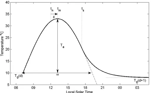
2 Theory

The time between solar noon and the time of the daily maximum is here referred to as 25

(6)

HESSD

10, 6019–6048, 2013

Title Page

Tables Figures

◭ ◮

Back Close

Full Screen / Esc

Discussion

P

a

per

|

Dis

cussion

P

a

per

|

Discussion

P

a

per

|

Discussio

n

P

a

per

|

eliminates any longitudinal dependency but also the smaller effect of variations in day length through the year. Accordingly, all times denoted here are given in local solar time.

For a surface temperature measurement, the averageφshould be directly related to the incoming radiation, with a delay (damping) that is a function of heat capacity of the 5

soil or vegetation layer over the measurement depth of the sensor. When comparing two temperature measurements with the same spatial extent, the measurement depth will determine the level of damping of the diurnal temperature cycle (Van Wijk and de Vries, 1963) and the measurement with the earliest peak will represent the shal-lowest layer. TIR measurements have a sensing depth of about 50 µm, providing the 10

shallowest practical measurement of LST. The timing of the maximum TIR temperature is typically reported between 60–90 min after solar noon (Choudhury et al., 1987; Betts and Ball, 1995; Fiebrich et al., 2003). Ka-band microwave emission has been shown to be a plausible alternative to TIR measurements, with much higher tolerance for clouds but a limited spatial resolution (Holmes et al., 2009). The sensing depth for Ka-band 15

microwave emission is slightly deeper than TIR and varies with soil moisture. For most land surfaces it is assumed to be around 1 mm. Accordingly, theφ derived from Ka-band emission is expected to be slightly behind that observed using TIR. Only in very dry areas with no vegetation is the Ka-band sensing depth potentially much deeper, in the order of cm’s (Ulaby et al., 1986), and theφof Ka-band can be even more delayed. 20

To illustrate the difference, a numerical example is given in Table 1 comparing a wet soil to a dry soil. The damping of the temperature harmonic with a period of a day can be described by a phase shift (dφ) proportional to the vertical distance (dz) divided by the damping depth (zD). The damping depth is defined as the dzover which the amplitude

of the harmonic is reduced by 63 %, and is an expression of the thermal properties of 25

the soil:

zD=

r 2a

2πf (1)

(7)

HESSD

10, 6019–6048, 2013

Title Page

Tables Figures

◭ ◮

Back Close

Full Screen / Esc

Discussion

P

a

per

|

Dis

cussion

P

a

per

|

Discussion

P

a

per

|

Discussio

n

P

a

per

|

whereais the thermal diffusivity (m2s−1) andf is the frequency (s−1) of the harmonic. For a dry soil (a=0.15e−6

) Eq. (1) yields an estimate ofzD=6.5 cm. Estimates of the

temperature sensing depth (zS) of 1 mm for a wet soil to 1 cm for a dry soil are given

in Ulaby et al. (1986). The difference in zS for microwave Ka-band emission between

a dry sandy soil and a wet soil is therefore about 9 mm. Dividing this by the dry soilzD

5

of 6.5 cm equates to a 3 h 36 min shift inφbetween the soil layers at the lower ends of these sensing depths (dφz). Because the shallower soil depths weigh more heavily in the measured emission, and they have larger diurnal amplitudes, they affect the timing of the DTC more strongly. Therefore, the shift in phase (dφ) of actual measured Ka-band emission, originating from the entire soil profile, is estimated at a fourth of dφz: 10

54 min. Observational evidence of this dφwill be discussed in Sect. 5.

3 Materials

In this study we compare three independent land temperature measurements, two from satellite measurements and one based on a global NWP model. The satellite obser-vations include a number of Ka-band sensors with global coverage, and TIR measure-15

ments from a geostationary satellite. All sets were available for the full year 2009 and are described below.

3.1 Satellite Ka-band brightness temperature

Vertical polarized Ka-band (37 GHz) brightness temperatures (T_BKa, V) observations are available from several satellites. For 2009 we acquired observations from the Ad-20

(8)

HESSD

10, 6019–6048, 2013

Title Page

Tables Figures

◭ ◮

Back Close

Full Screen / Esc

Discussion

P

a

per

|

Dis

cussion

P

a

per

|

Discussion

P

a

per

|

Discussio

n

P

a

per

|

resolution and the location of the center of the footprint and its azimuth orientation varies between consecutive overpasses. To combine these observations, they are binned to a 0.25◦ regular global grid. This resolution was chosen based on the satel-lite with the coarsest resolution (SSM/I, see Table 2). The value for each grid cell is the mean of all observations with a footprint center within the boundaries of the cell. 5

The inter-calibration of these five instruments makes use of the precessing nature of TRMM’s equatorial orbit. This orbit was designed to sample the diurnal variation of tropical rainfall and results in regular overlap with all polar orbiting satellites, allowing for an inter-calibration of the satellites as described in Holmes et al. (2013).

Within the microwave spectrum,T_BKa, Vis the most appropriate frequency to retrieve 10

LST as it balances a reduced sensitivity to soil surface characteristics with a relatively high atmospheric transmissivity (Colwell et al., 1983). In Holmes et al. (2009) it was further shown that an assumption of a constant land surface emissivity can be used to obtain LST estimates from Ka-band with relatively high sensitivity, if not absolute ac-curacy. For the purpose of this paper no conversion to physical temperature is needed 15

since only the timing of the DTC is analysed here, not its amplitude. This means that for this paper the assumption of constant emissivity needs only to hold over the course of the day, and that there is no e_ffect of absolute bias in LST on the analysis. Still, the linear relationship between Ka-band and LST does potentially break down under frozen soil conditions or during precipitation events. This leads to the formulation of two 20

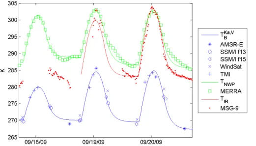
conditions for the Ka-band data:T_BKa, V>260 K, andσKa, V<mean(σKa, V), as explained in more detail in Holmes et al. (2013). The Ka-band temperature set is referred to in the following asTKa. An example of the resulting sampling of the combinedTKais given

in Fig. 1 for three days in September 2009. In the same graph the NWP and infrared resource are shown, they are described below.

25

(9)

HESSD

10, 6019–6048, 2013

Title Page

Tables Figures

◭ ◮

Back Close

Full Screen / Esc

Discussion

P

a

per

|

Dis

cussion

P

a

per

|

Discussion

P

a

per

|

Discussio

n

P

a

per

|

3.2 NWP surface temperature

The modeled temperature dataset was acquired from NASA’s Global Modeling and Assimilation Office (GMAO) and their Modern Era Retrospective-analysis for Re-search and Applications (MERRA) (http://gmao.gsfc.nasa.gov/reRe-search/merra, Rie-necker et al., 2011). MERRA products are generated using Version 5.2.0 of the GEOS-5

5 DAS (Goddard Earth Observing System (GEOS) Data Assimilation System (DAS)) with the analysis and model output both at a spatial resolution of 0.5◦ latitude by 0.67◦ longitude, and with a 6 hourly analysis cycle. Two dimensional diagnostics describing the radiative and physical state of the surface are available as hourly averages.

Surface processes in MERRA are based on the NASA Catchment land surface 10

model (Ducharne et al., 2000; Koster et al., 2000). Each MERRA grid cell contains sev-eral irregularly shaped tiles, and each tile is further divided into sub-tiles based on their modeled hydrological state: saturated, unsaturated, and wilting. The surface tempera-ture of a grid cell is obtained by area-weighted averaging of the surface temperatempera-tures of all sub-tiles within the grid cell. The sub-tile surface temperatures are prognostic 15

variables of the model and represent a bulk surface layer with a small but finite heat capacity. For all vegetation classes except broadleaf evergreen trees, this bulk surface layer represents the vegetation canopy and a surface layer at the top of the soil column (effective layer depth<1 mm).

In this study we analyzed the gridded surface temperatures over land, orTNWP. The

20

data was regridded onto a 0.25◦ regular grid by means of bilinear interpolation, and the hourly output was temporally interpolated to a 15 min temporal resolution. Figure 1 gives an example ofTNWPat the original hourly resolution.

3.3 Geostationary thermal infrared based LST

TIR-based land surface temperature from METEOSAT-9 with coverage over Africa 25

and Europe was available as a third independent data source. LST (TIR) is an

(10)

HESSD

10, 6019–6048, 2013

Title Page

Tables Figures

◭ ◮

Back Close

Full Screen / Esc

Discussion

P

a

per

|

Dis

cussion

P

a

per

|

Discussion

P

a

per

|

Discussio

n

P

a

per

|

see http://landsaf.meteo.pt). It is generated using spinning enhanced visible and infra red imager (SEVIRI) split-window channels (10.8 and 12.0 µm) on board the geosta-tionary Meteosat second generation (MSG) satellite; therefore a high temporal resolu-tion (15 min) of the data is possible (Kabsch et al., 2008; Trigo et al., 2011).

This LST data is provided on a 3-km equal area grid. When regridding onto a 0.25◦ 5

regular grid, this results in a large over sampling of the grid box. If more than two-thirds of the 3-km observations are masked out for a particular location and time, then that sampling average is rejected. This threshold increases the amount of data discarded by the cloud filter forTIR. We further limit the coverage of the METEOSAT-9 to the domain

covered with an Earth incidence angle of 78◦, avoiding artifacts at large view angles. 10

In Fig. 1 the high sampling rate ofTIRis apparent, as are gaps (attributed to clouds) on

day 1 and 2 of this example series.

4 Methods

In Holmes et al. (2012) it was shown that a relative estimate ofφcan be determined by fitting a simple harmonic model to a temperature time-series. This worked well enough 15

when onlyφdifferences between temperature sets are needed. However, the values itself are hard to interpret since the actual shape of the DTC rarely resembles a perfect harmonic shape resulting in differences between the time of maximum temperature and the peak of the harmonic.

In this paper we adapt a more sophisticated model of the DTC as described by 20

G ¨ottsche and Olesen (2001). This harmonic-exponential DTC model improves the fit along the cooling limb of the DTC and allows for better leveraging of observations at all times. In addition, it yields an estimate ofφthat can be more readily interpreted as the time-lag between solar noon and peak temperature. The DTC model by G ¨ottsche and Olesen (2001) is originally intended as a five parameter model, and a subsequent ad-25

dition to parameterize total (atmospheric) optical depth increased this to six (G ¨ottsche and Olesen, 2009). A recent comparison paper (Duan et al., 2012) discussed several

(11)

HESSD

10, 6019–6048, 2013

Title Page Abstract Introduction Conclusions References Tables Figures ◭ ◮ ◭ ◮ Back Close

Full Screen / Esc

Printer-friendly Version Interactive Discussion Discussion P a per | Dis cussion P a per | Discussion P a per | Discussio n P a per |

variants of the DTC model by G ¨ottsche and Olesen (2001) and showed that improve-ments were caused by adding an additional free parameter related to the day-length. In this paper we have to reduce the number of free parameters to limit the computational demands and speed conversion to a solution. Therefore we simplify the five parameter model (G ¨ottsche and Olesen, 2001) to have only three free parameters. A test shows 5

that this does not reduce the accuracy of the meanφas determined over longer time series. The method is detailed below.

In G ¨ottsche and Olesen (2001) the DTC model (Tpar) is parameterized as a function

of the time of maximum (tm), day length (ω), diurnal amplitude (Ta), diurnal minimum

(T0), change in minimum from day to day (δT), and start of the attenuation function (ts):

10

Tpar(t)=T0+Tacos

π

ω(t−tm)

, t < ts (2)

Tpar(t)=T0+δT+

h Tacos

π

ω(ts−tm)

−δT i

e−(tk−ts), t≥t_s

Figure 2 shows an example ofTpar, and illustrates the definitions of its parameters.

The attenuation constantk is calculated by making the first derivatives of the day and 15

night time equation equal at timets:

k=_ωπ

"

1 tan _ωπ(ts−tm)

−

δT Tasin ωπ(ts−tm)

#

(3)

To limit the degrees of freedom and increase conversion to a solution, in this study the start of the attenuation function is fixed so that half of the decrease in temperature (over the cooling down limb) is described by the exponential equation. That way,tscan

20

be calculated fromtmandωas:

ts=tm+

ω πarccos 1 2 1+δT

T_a

(4)

For a given day and temperature set, first guess estimates of T0 and Ta are

(12)

HESSD

10, 6019–6048, 2013

Title Page

Tables Figures

◭ ◮

Back Close

Full Screen / Esc

Discussion

P

a

per

|

Dis

cussion

P

a

per

|

Discussion

P

a

per

|

Discussio

n

P

a

per

|

period from sunrise to sunrise. Similarly,δT is initialized based on the difference be-tweenT0of the current and the next day, if available. Solar noon (tn) andωare

calcu-lated based on latitude and day of year according to general solar position calculations Cornwall et al. (2003). Definingφ as the offset between optimized time of maximum temperature and sunrise tm=tn+φ, there are three free parameters: φ, T0, Ta. Of

5

these, onlyT0, Ta, vary from day to day,φ is assumed constant over the data range.

With these assumptions it is possible to determineφ in an iterative optimization loop that minimizes the squared errors (E) betweenTpar and the data series. In Fig. 1

ex-amples ofTparare shown, as fitted for the three LST resources used in this manuscript.

The timing of the DTC can be determined if temperature observations are available 10

with a su_fficient sampling, which at minimum includes samples near the time of mini-mum and maximini-mum temperature and at mid morning and afternoon. Furthermore, days (d) where one of the following conditions are not met are removed from the timing fitting to assure that the basic assumptions of the temperature model are not violated:

1. T0(d) above freezing point,

15

2. tm(d) within 2 h of meantm,

3. Ta>5 K, and

4. N(d)>median(N(d=1 : end)).

The first condition is used to avoid days with subfreezing temperatures because the Ka-band/LST relationship weakens under these circumstances, and the second as-20

sures that the DTC has a shape close to the clear sky assumptions. The third condition is intended to make sure the signal to noise ratio is acceptable. The last condition tests that the sampling of the DTC is not much less than on the average day (N(d) is the number of datapoints in LST at dayd).

The fitting of the timing is dependent on the sampling of the series. To test if the 25

sampling ofTKaresults in a bias relative to the hourly sampling of MERRA, we looked at

the change in apparent timing forTNWP, when only observations at the overpass times

(13)

HESSD

10, 6019–6048, 2013

Title Page

Tables Figures

◭ ◮

Back Close

Full Screen / Esc

Discussion

P

a

per

|

Dis

cussion

P

a

per

|

Discussion

P

a

per

|

Discussio

n

P

a

per

|

of the Ka-band set are used. The effect of sparse sampling on theφ is averaged by latitude and shown in Fig. 3. The e_ffect was no greater than 9 min for 99 % of the data, although on average the sparse sampling resulted in 2 min positive bias ofφ. These results indicate that the uncertainty as introduced by the limited sampling frequency of the Ka-band data is small enough to measure Ka-band timing from this set of sensors. 5

5 Results

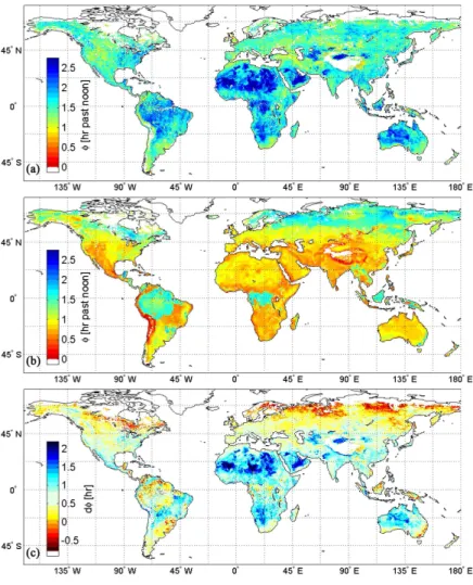
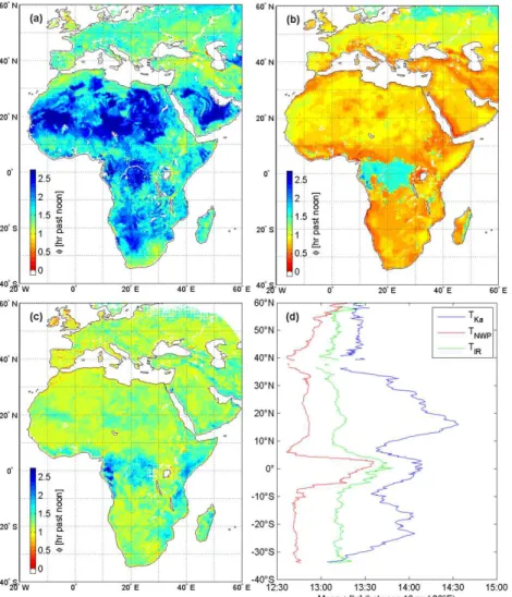
The above described method to determine φ is applied to the three temperature recordsTKa, TNWP, and TIR (described in Sect. 3) for the data year 2009. The

result-ing (0.25◦) maps ofφare displayed in Fig. 4 for Europe and Africa, the spatial domain of MSG-9.

10

On average theTKapeaks at 13:44 with lower values over Europe and highest

val-ues over deserts and tropical rainforests. Later valval-ues of peak temperature in deserts can be explained by the deeper sensing depth of Ka-band emission under dry soil conditions (see Sect. 2). In fact, the areas with latest φ correspond closely to sand deserts, see for example the Arabian Peninsula in Fig. 4a where the Rub’al Khali Erg 15

shows up causing an hour delay of the Ka-bandφ. This feature was earlier noted in terms of day/night di_fference of SSM/I channels (Prigent et al., 1999), polarization dif-ference of AMSR-E channels (Jim ´enez et al., 2010), and even more comparable to the present analysis, in terms of phase difference between microwave and TIR temperature (Norouzi et al., 2012). In this later study the third component derived from a principal 20

component analysis (PCA) was attributed to the phase of the diurnal cycle. The close resemblance of the spatial features generally supports this conclusion.

Another feature in the maps ofφ(TKa) is the earlier phase over mountainous areas

(e.g. the Rif mountains in NW Africa, Caucasus). Since TKa is composed of

obser-vations with varying azimuth angles, the signature likely reflects a deviation in actual 25

(14)

HESSD

10, 6019–6048, 2013

Title Page

Tables Figures

◭ ◮

Back Close

Full Screen / Esc

Discussion

P

a

per

|

Dis

cussion

P

a

per

|

Discussion

P

a

per

|

Discussio

n

P

a

per

|

For TNWP, with a mean peak temperature at 12:50, there is much less spatial

vari-ation inφ with the notable exception of tropical rainforest, see Fig. 4b. The distinctly different results over rainforest with values around 13:30 are explained by a higher heat capacity as parameterized for areas classified as tropical forest in the MERRA model. At more northern latitudes, higherφ-values are found over the forest areas of 5

the East-European plain.

Figure 4c shows theφas determined based onTIR. TheTIRdata peak on average at

13:13. The higherφ-values in the tropical zone match well with the delay as found for TNWP, although forTIRthe area with delayedφis slightly more expansive and includes

more generally the humid tropical zone of Africa. 10

Figure 4d shows a North South transect of theφ as determined forTKa,TNWP, and

TIR; all averaged over the longitude extent of 0–30

◦

E. All sets have a delayedφaround the equator, which forTNWPis explained by the higher heat-capacity as parameterized

for tropical rainforest. ForT_KaandT_IR, with little to none penetration of the canopy layer, the delay in φ might more plausibly have to do with the effect of a diurnal pattern 15

in cloudiness which can cause a delay in the peak solar radiation. Superimposed on this tropical signature, T_Ka clearly shows a delayed φ over (seasonally) dry areas in Northern and Southern Africa, explained by the deeper sensing depth.

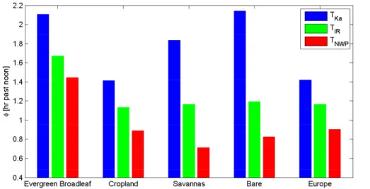
Some of the patterns in φ and differences between the sets seem to align with particular land surface types. Therefore, MODIS land cover maps (MCD12C1, Version 20

051) are used to study φ by land surface type (International Geosphere-Biosphere Programme (IGBP) classification). Figure 6 lists the average values as obtained over selected surface types between longitudes 0 to 30◦E. This indeed confirms the general relation with vegetation type; bothTIRandTNWPexhibit delayedφover broadleaf forest

compared to all other land surface types. As a consequence, the mean difference inφ 25

is remarkably homogenous:φ(TIR)−φ(TNWP)=27 min (±15 min) for 79 % of the land

area. Areas with larger di_fferences are found at the edge of land masses whereφ(TIR)

can be up to 1.5 h behindφ(TNWP) as shown in Fig. 5. This is apparently related toTIR

exhibiting a delay inφrelative to the interior of the continents (see also Fig. 4c). Since

(15)

HESSD

10, 6019–6048, 2013

Title Page

Tables Figures

◭ ◮

Back Close

Full Screen / Esc

Discussion

P

a

per

|

Dis

cussion

P

a

per

|

Discussion

P

a

per

|

Discussio

n

P

a

per

|

these features appear to line up with the mountain ranges, with delayedφover ranges that are to the East of MSG-9, and earlierφover mountains to the North-West of the satellite, it is tentatively attributed to orographic effects as described in Senkova et al. (2007).

Although TKa closely matches TIR in terms of φ for the forest and cropland cover

5

types, an additional delay is recorded over the dry areas of the world, as is evident in Figs. 4 and 6. The resulting timing difference between TKa andTIR is therefore

great-est over the drigreat-est parts of Africa, whereTKais 57 min (±25 min) behindTIR inφ, see

Fig. 5b. This average dφagrees with the theoretical calculations of Sect. 4. This sug-gests that the large increase in φKa over dry areas can be quantitatively explained

10

by the increase in temperature sensing depth. As expected for all but the driest soils (especially when covered with vegetation) the difference is much closer to zero over the rest of Africa and Europe. For example, over Europe theφ-maps show thatTKais

only 14 min (±12 min) behindTIR. In some coastal and mountainous areas theφ-maps

indicate thatTKa peaks earlier thanTIR, which is not physically realistic. Most of these

15

areas also show up in the previous discussion of Fig. 5a, and are attributed to a delay inTIR that has yet to be fully explained. It is most likely related to a failure of the cloud

mask applied to TIR. In addition to those areas however,TKa appears to be ahead of

TIR over Turkey and this is likely caused by TKa, which has anomalous early φ there

(see Fig. 4a). The difference inφbetweenTKaandTNWP will be discussed in a global

20

context in the next section.

It is investigated if these patterns inφare stable through the year. For that the above procedure was repeated for 3 month seasonal periods. ForTKaandTNWPno differences

with the annualφwere found larger than 15 min. ForTIRthe northern sub-tropical zone

showed delayedφ of up to a half hour, but this is likely related to a lack of sufficient 25

(16)

HESSD

10, 6019–6048, 2013

Title Page

Tables Figures

◭ ◮

Back Close

Full Screen / Esc

Discussion

P

a

per

|

Dis

cussion

P

a

per

|

Discussion

P

a

per

|

Discussio

n

P

a

per

|

6 Global results

This section will briefly discuss the global maps ofφ as generated for TKaand TNWP.

The geostationary TIR resource is not yet available as a consolidated global dataset and is therefore not included here.

The global maps ofφconfirm the land-cover features as discussed above. TheTKa

5

peaks on average at 13:37 (see Fig. 7, top), but over desert areas this peak is up to an hour delayed. ForTNWP (Fig. 7, middle panel), φ is generally between 12:30 and

13:00 with two main exceptions, the tropical regions and Northern latitudes. Highly delineated areas appear in the tropical zone with a delay in φ of up about 40 min. As discussed earlier, this is explained by the increased heat capacity of the surface 10

layer as parameterized for tropical forest by MERRA. Because this is a static feature of MERRA, the resulting spatial pattern ofφis expected to remain stable from year to year, as long as the same land classification is used. Above 60◦N delays of up to an hour are calculated (e.g. Alaska, Scandinavia, Siberia) possibly resulting from frozen circumstances and a less pronounced diurnal temperature range.

15

On averageTKapeaks 40 min later thanTNWP (Fig. 7, lower pane). In the temperate

climates and the tropics the dφis close to this average. Bigger differences appear in the desert areas where Ka-band peaks up to 2 h afterTNWP, corresponding to a deeper

sensing depth. The Northern latitudes show smaller di_fferences due to the delayedφ ofTNWP, a feature that is not matched inTKa. Due to the close link with land cover and

20

geological features it is expected that these patterns of dφwould largely remain stable from year to year.

7 Conclusions

This study has demonstrated that the timing of the diurnal temperature cycle can reli-ably be determined from temporally sparse datasets. The method is applied to a year-25

long record of geostationary TIR observations, model output, and a combination of low

(17)

HESSD

10, 6019–6048, 2013

Title Page

Tables Figures

◭ ◮

Back Close

Full Screen / Esc

Discussion

P

a

per

|

Dis

cussion

P

a

per

|

Discussion

P

a

per

|

Discussio

n

P

a

per

|

Earth orbiting satellites with microwave radiometers. The spatial patterns inφfor each temperature set are explainable based on consideration of land surface type and ba-sic phyba-sics describing the penetration depth of microwave observations. An interesting observation is that over tropical forest the timing is delayed by 30 to 40 min relative to the average phase in both satellite data sets. While this delay is accurately modeled in 5

MERRA, it may be for the wrong reason if the delay is caused by a diurnal variability of cloudiness rather than an increase in heat capacity of the sampled surface layer. On the other hand, deserts cause a delay in the timing of Ka-band diurnal temperature cy-cle that is not matched in the TIR nor MERRA estimates. This is explained by a deeper sensing depth for the microwave observations in dry soils, and becomes especially 10

extreme in dry sand deserts.

In absolute terms, MERRA seems to model the peak of the DTC about 23 min before that of TIR, which should be the shallowest observation possible of the land surface. Therefore, if the goal is to model the surface temperature it appears the heat capacity of the surface layer is set slightly too low in MERRA. The timing of Ka-band observations 15

outside of the desert areas is on average 15 min after TIR. This small delay of the DTC compared to TIR agrees with a slightly deeper sensing depth for Ka-band, 50 µm vs. 1 mm.

This study has identified structural differences in diurnal timing between MERRA, TIR and Ka-band based land surface temperature estimates and constitutes one of 20

the first global analyses of the effects of vegetation and sensing depth on the timing of different temperature measurements. Even though the global maps of the timing for each set are based on the year 2009, these features are expected to be relatively stable from year to year. With these maps we can now attempt to adjust for these structural differences in temperature estimates and study the relative merit of each method in 25

a more consistent way.

(18)

HESSD

10, 6019–6048, 2013

Title Page

Tables Figures

◭ ◮

Back Close

Full Screen / Esc

Discussion

P

a

per

|

Dis

cussion

P

a

per

|

Discussion

P

a

per

|

Discussio

n

P

a

per

|

Flight Center) for the dissemination of MERRA. USDA is an equal opportunity provider and employer.

References

Anderson, M. C., Norman, J. M., Diak, G. R., Kustas, W. P., and Mecikalski, J. R.: A two-source time-integrated model for estimating surface fluxes using thermal infrared remote sensing,

5

Remote Sens. Environ., 60, 195–216, 1997. 6023

Anderson, M. C., Hain, C., Wardlow, B., Pimstein, A., Mecikalski, J. R., and Kustas, W. P.: Evaluation of drought indices based on thermal remote sensing of evapotranspiration over the continental United States, J. Climate, 24, 2025–2044, doi:10.1175/2010jcli3812.1, 2011. 6021

10

Bauer, P., Aulign ´e, T., Bell, W., Geer, A., Guidard, V., Heilliette, S., Kazumori, M., Kim, M. J., Liu, E. H. C., and McNally, A. P.: Satellite cloud and precipitation assimilation at operational NWP centres, Q. J. Roy. Meteor. Soc., 137, 1934–1951, 2011. 6020

Betts, A. K. and Ball, J. H.: The FIFE surface diurnal cycle climate, J. Geophys. Res.-Atmos., 100, 25679–25693, 1995. 6024

15

Bosilovich, M. G., Radakovich, J. D., da Silva, A., Todling, R., and Verter, F.: Skin tempera-ture analysis and bias correction in a coupled land-atmosphere data assimilation system, J. Meteorol. Soc. Jpn., 85, 205–228, 2007. 6021

Choudhury, B. J., Idso, S. B., and Reginato, R. J.: Analysis of an empirical model for soil heat flux under a growing wheat crop for estimating evaporation by an infrared-temperature based

20

energy balance equation, Agr. Forest Meteorol., 39, 283–297, 1987. 6024

Colwell, R. N., Simonett, D. S., and Ulaby, F. T. (Eds.): Manual of remote sensing, in: Interpre-tation and Applications, 2nd Edn., vol. II, Falls Church, 1983. 6026

Cornwall, C., Horiuchi, A., and Lehman, C.: General solar position calculations., available at: http://www.esrl.noaa.gov/gmd/grad/solcalc/solareqns.PDF (last access: May 2013), 2003.

25

6030

Dai, A. and Trenberth, K. E.: The diurnal cycle and its depiction in the Com-munity Climate System Model, J. Climate, 17, 930–951, doi:10.1175/1520-0442(2004)017<0930:TDCAID>2.0.CO;2, 2004. 6022

(19)

HESSD

10, 6019–6048, 2013

Title Page

Tables Figures

◭ ◮

Back Close

Full Screen / Esc

Discussion

P

a

per

|

Dis

cussion

P

a

per

|

Discussion

P

a

per

|

Discussio

n

P

a

per

|

Duan, S.-B., Li, Z.-L., Wang, N., Wu, H., and Tang, B.-H.: Evaluation of six land-surface diurnal temperature cycle models using clear-sky in situ and satellite data, Remote Sens. Environ., 124, 15–25, 2012. 6028

Ducharne, A., Koster, R., Suarez, M., Stieglitz, M., and Praveen, K.: A catchement-based ap-proach to modeling land-surface processes in a GCM – 2. Parameter estimation and model

5

demonstration, J. Geophys. Res., 105, 24809–24822, 2000. 6027

Fiebrich, C. A., Martinez, J. E., Brotzge, J. A., and Basara, J. B.: The Oklahoma Mesonet’s Skin Temperature Network, J. Atmos. Ocean. Tech., 20, 1496–1504, doi:10.1175/1520-0426(2003)020<1496:TOMSTN>2.0.CO;2, 2003. 6024

G ¨ottsche, F.-M. and Olesen, F. S.: Modelling of diurnal cycles of brightness temperature

ex-10

tracted from METEOSAT data, Remote Sens. Environ., 76, 337–348, 2001. 6028, 6029 G ¨ottsche, F.-M. and Olesen, F.-S.: Modelling the effect of optical thickness on diurnal cycles of

land surface temperature, Remote Sens. Environ., 113, 2306–2316, 2009. 6028

Hain, C. R., Anderson, M. C., Zhan, X., Svoboda, M., Wardlow, B., Mo, K., Meckalski, J. R., Kustas, W. P., and Brown, J.: A GOES Thermal-Based Drought Early Warning Index for

15

NIDIS, in: NOAA’s National Weather Service, Science and Techn. Inf. Climat. B., Fort Worth, TX, 2011. 6021

Holmes, T. R. H., De Jeu, R. A. M., Owe, M., and Dolman, A. J.: Land surface temperature from Ka band (37 GHz) passive microwave observations, J. Geophys. Res., 114, D04113, doi:10.1029/2008JD010257, 2009. 6024, 6026

20

Holmes, T. R. H., Jackson, T. J., Reichle, R. H., and Basara, J. B.: An assessment of surface soil temperature products from numerical weather prediction models using ground-based measurements, Water Resour. Res., 48, W02531, doi:10.1029/2011WR010538, 2012. 6022, 6028

Holmes, T. R. H., Crow, W. T., Yilmaz, M. T., Jackson, T. J., and Basara, J. B.: Enhancing

model-25

based land surface temperature estimates using multiplatform microwave observations, J. Geophys. Res.-Atmos., 118, 1–15, 2013. 6022, 6026

Jim ´enez, C., Catherinot, J., Prigent, C., and Roger, J.: Relations between geological character-istics and satellite-derived infrared and microwave emissivities over deserts in northern Africa and the Arabian Peninsula, J. Geophys. Res., 115, D20311, doi:10.1029/2010JD013959,

30

(20)

HESSD

10, 6019–6048, 2013

Title Page

Tables Figures

◭ ◮

Back Close

Full Screen / Esc

Discussion

P

a

per

|

Dis

cussion

P

a

per

|

Discussion

P

a

per

|

Discussio

n

P

a

per

|

Kabsch, E., Olesen, F. S., and Prata, F.: Initial results of the land surface temperature (LST) validation with the Evora, Portugal ground-truth station measurements, Int. J. Remote Sens., 29, 5329–5345, doi:10.1080/01431160802036326, 2008. 6028

Koster, R., Suarez, M., Ducharne, A., Stieglitz, M., and Praveen, K.: A catchement-based ap-proach to modeling land-surface processes in a GCM – 1. Model structure, J. Geophys. Res.,

5

105, 24809–24822, 2000. 6027

Norouzi, H., Tenimi, M., AghaKouchak, A., Azarderakhsh, M., and Khanbilvardi, R.: On the effect of land cover type on the diurnal cycle of microwave brightness tmperatures, IEEE Geosci. Remote Sense., submitted, 2012. 6031

Parinussa, R. M., Holmes, T. R. H., and De Jeu, R. A. M.: Soil moisture retrievals from the

10

WindSat spaceborne polarimetric microwave radiometer, IEEE Trans. Geosci. Remote, 50, 2683–2694, doi:10.1109/TGRS.2011.2174643, 2012. 6021

Prigent, C., Rossow, W. B., Matthews, E., and Marticorena, B.: Microwave radiometric signatures of di_fferent surface types in deserts, J. Geophys. Res., 104, 12147–12158, doi:10.1029/1999JD900153, 1999. 6031

15

Reichle, R. H., Kumar, S. V., Mahanama, S. P. P., Koster, R. D., and Liu, Q.: Assimilation of satellite-derived skin temperature observations into land surface models, J. Hydrol., 11, 1103–1122, doi:10.1175/2010JHM1262.1, 2010. 6021

Rienecker, M. M., Suarez, M. J., Gelaro, R., Todling, R., Bacmeister, J., Liu, E., Bosilovich, M. G., Schubert, S. D., Takacs, L., Kim, G.-K., Bloom, S., Chen, J., Collins, D.,

20

Conaty, A., da Silva, A., Gu, W., Joiner, J., Koster, R. D., Lucchesi, R., Molod, A., Owens, T., Pawson, S., Pegion, P., Redder, C. R., Reichle, R., Robertson, F. R., Ruddick, A. G., Sienkiewicz, M., and Woollen, J.: MERRA: NASA’s Modern-Era Retrospective Analysis for Research and Applications, J. Climate, 24, 3624–3648, doi:10.1175/JCLI-D-11-00015.1, 2011. 6027

25

Rosnay, P. D., Drusch, M., Balsamo, G., Albergel, C., and Isaksen, L.: Extended Kalman Filter soil-moisture analysis in the IFS, ECMWF Newsletter, pp. 12–15, available at: http://www. ecmwf.int/publications/newsletters/pdf/127.pdf (last access: May 2013), 2011. 6021

Senkova, A. V., Rontu, L., and Savijarvi, H.: Parametrization of orographic e_ffects on surface radiation in HIRLAM, Tellus A, 59, 279–291, doi:10.1111/j.1600-0870.2007.00235.x, 2007.

30

6033

Smith, E., Asrar, G., Furuhama, Y., Ginati, A., Mugnai, A., Nakamura, K., Adler, R., Chou, M. D., Desbois, M., and Durning, J.: International global precipitation measurement (GPM) program

(21)

HESSD

10, 6019–6048, 2013

Title Page

Tables Figures

◭ ◮

Back Close

Full Screen / Esc

Discussion

P

a

per

|

Dis

cussion

P

a

per

|

Discussion

P

a

per

|

Discussio

n

P

a

per

|

and mission: an overview, in: Measuring Precipitation From Space, Springer, 611–653, 2007. 6022

Stephens, G. L. and Kummerow, C. D.: The remote sensing of clouds and precipitation from space: a review, J. Atmos. Sci., 64, 3742–3765, doi:10.1175/2006JAS2375.1, 2007. 6023 Trigo, I. F., Dacamara, C. C., Viterbo, P., Roujean, J. L., Olesen, F., Barroso, C.,

5

Camacho-de Coca, F., Carrer, D., Freitas, S. C., and Garcia-Haro, J.: The satellite application facility for land surface analysis, Int. J. Remote Sens., 32, 2725–2744, doi:10.1080/01431161003743199, 2011. 6028

Ulaby, F. T., Moore, R. K., and Fung, A. K.: From theory to applications, in: Microwave Remote Sensing: Active and Passive, vol. III, Artech House, Norwood, MA, 1986. 6024, 6025

10

(22)

HESSD

10, 6019–6048, 2013

Title Page

Tables Figures

◭ ◮

Back Close

Full Screen / Esc

Discussion

P

a

per

|

Dis

cussion

P

a

per

|

Discussion

P

a

per

|

Discussio

n

P

a

per

|

Table 1.Soil thermal properties and phase shift examples.

Wet soil Dry soil

a: thermal diffusivity (m2s−1) 0.56e−6

0.15e−6

z_D: damping depth (m) 0.124 0.064 z_S: sensing depth (m) 0.001 0.01

dφz: phase shift between dφz=(zS, dry−zS, moist)/zD

deepest layers, wet to dry =(0.009/0.06)=3 h 36 min

dφ: effective phase shift dφ=dφz/4=54 min

(23)

HESSD

10, 6019–6048, 2013

Title Page

Tables Figures

◭ ◮

Back Close

Full Screen / Esc

Discussion

P

a

per

|

Dis

cussion

P

a

per

|

Discussion

P

a

per

|

Discussio

n

P

a

per

|

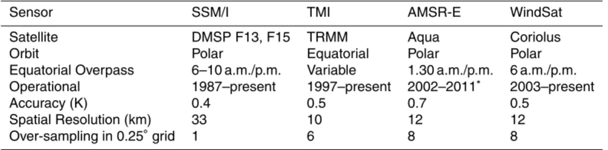
Table 2.Specifications of satellite sensors providing Ka-band microwave observations used for land surface temperature estimation. (∗AMSR2 was launched in May 2012.)

Sensor SSM/I TMI AMSR-E WindSat

Satellite DMSP F13, F15 TRMM Aqua Coriolus

Orbit Polar Equatorial Polar Polar

Equatorial Overpass 6–10 a.m./p.m. Variable 1.30 a.m./p.m. 6 a.m./p.m.

Operational 1987–present 1997–present 2002–2011∗

2003–present

Accuracy (K) 0.4 0.5 0.7 0.5

Spatial Resolution (km) 33 10 12 12

(24)

HESSD

10, 6019–6048, 2013

Title Page

Tables Figures

◭ ◮

Back Close

Full Screen / Esc

Discussion

P

a

per

|

Dis

cussion

P

a

per

|

Discussion

P

a

per

|

Discussio

n

P

a

per

|

Fig. 1.Three days of diurnal cycles ofT_Ka,T_NWP, andT_IRin September 2009. All variables are explained in Sect. 3. Solid lines represent the fitted DTC, as described in Sect. 4.

(25)

HESSD

10, 6019–6048, 2013

Title Page

Tables Figures

◭ ◮

Back Close

Full Screen / Esc

Discussion

P

a

per

|

Dis

cussion

P

a

per

|

Discussion

P

a

per

|

Discussio

n

P

a

per

|

(26)

HESSD

10, 6019–6048, 2013

Title Page

Tables Figures

◭ ◮

Back Close

Full Screen / Esc

Discussion

P

a

per

|

Dis

cussion

P

a

per

|

Discussion

P

a

per

|

Discussio

n

P

a

per

|

Fig. 3.Effect of sparse sampling on retrieval ofφ, tested atT_Kaobservation times.

(27)

HESSD

10, 6019–6048, 2013

Title Page

Tables Figures

◭ ◮

Back Close

Full Screen / Esc

Discussion

P

a

per

|

Dis

cussion

P

a

per

|

Discussion

P

a

per

|

Discussio

n

P

a

per

|

(28)

HESSD

10, 6019–6048, 2013

Title Page

Tables Figures

◭ ◮

Back Close

Full Screen / Esc

Discussion

P

a

per

|

Dis

cussion

P

a

per

|

Discussion

P

a

per

|

Discussio

n

P

a

per

|

Fig. 5.Timing difference [h]:(a)φ(T_NWP)−φ(T_IR), average dφ=−23 min, and(b)φ(T_Ka)−φ(T_IR), average dφ=30 min. Color bar centered on the average for each map.

(29)

HESSD

10, 6019–6048, 2013

Title Page

Tables Figures

◭ ◮

Back Close

Full Screen / Esc

Discussion

P

a

per

|

Dis

cussion

P

a

per

|

Discussion

P

a

per

|

Discussio

n

P

a

per

|

Fig. 6.2009 mean φdetermined for TKa,TIR, andTNWP for selected IGBP land-cover types.

BetweenTNWP and TIR there is a fairly constant dφof 20 min.TKa agrees with TIR over land

(30)

HESSD

10, 6019–6048, 2013

Title Page

Tables Figures

◭ ◮

Back Close

Full Screen / Esc

Discussion

P

a

per

|

Dis

cussion

P

a

per

|

Discussion

P

a

per

|

Discussio

n

P

a

per

|

Fig. 7.2009 meanφforTKa(a),TNWP (b), and differenceTKa−TNWP(c).