A novel bias correction methodology for climate impact simulations

(1)

ESDD

6, 1999–2042, 2015

Ensemble bias correction

S. Sippel et al.

Title Page

Abstract Introduction

Conclusions References

Tables Figures

◭ ◮

Back Close

Full Screen / Esc

Printer-friendly Version Interactive Discussion

Discussion

P

a

per

|

Discussion

P

a

per

|

Discussion

P

a

per

|

Discussion

P

a

per

|

Earth Syst. Dynam. Discuss., 6, 1999–2042, 2015 www.earth-syst-dynam-discuss.net/6/1999/2015/ doi:10.5194/esdd-6-1999-2015

This discussion paper is/has been under review for the journal Earth System Dynamics (ESD). Please refer to the corresponding final paper in ESD if available.

A novel bias correction methodology for

climate impact simulations

S. Sippel1,2, F. E. L. Otto3, M. Forkel1, M. R. Allen3, B. P. Guillod3, M. Heimann1, M. Reichstein1, S. I. Seneviratne2, K. Thonicke4, and M. D. Mahecha1,5

1

Max Planck Institute for Biogeochemistry, Hans-Knöll-Str. 10, 07745 Jena, Germany

2

Institute for Atmospheric and Climate Science, ETH Zürich, Rämistr. 101, 8075 Zürich, Switzerland

3

Environmental Change Institute, University of Oxford, South Parks Road, Oxford, OX1 3QY, UK

4

Potsdam Institute for Climate Impact Research, Telegrafenberg, 14473 Potsdam, Germany

5

German Centre for Integrative Biodiversity Research (iDiv), Halle-Jena-Leipzig, Deutscher Platz 5E, 04103 Leipzig, Germany

Received: 24 September 2015 – Accepted: 3 October 2015 – Published: 19 October 2015

Correspondence to: S. Sippel (ssippel@bgc-jena.mpg.de)

(2)

ESDD

6, 1999–2042, 2015

S. Sippel et al.

Title Page

Tables Figures

◭ ◮

Back Close

Full Screen / Esc

Discussion

P

a

per

|

Discussion

P

a

per

|

Discussion

P

a

per

|

Discussion

P

a

per

|

Abstract

Understanding, quantifying and attributing the impacts of extreme weather and climate events in the terrestrial biosphere is crucial for societal adaptation in a changing cli-mate. However, climate model simulations generated for this purpose typically exhibit biases in their output that hinders any straightforward assessment of impacts. To

over-5

come this issue, various bias correction strategies are routinely used to alleviate climate model deficiencies most of which have been criticized for physical inconsistency and the non-preservation of the multivariate correlation structure. In this study, we intro-duce a novel, resampling-based bias correction scheme that fully preserves the phys-ical consistency and multivariate correlation structure of the model output. This

proce-10

dure strongly improves the representation of climatic extremes and variability in a large regional climate model ensemble (HadRM3P, climateprediction.net/weatherathome), which is illustrated for summer extremes in temperature and rainfall over Central Eu-rope. Moreover, we simulate biosphere–atmosphere fluxes of carbon and water using a terrestrial ecosystem model (LPJmL) driven by the bias corrected climate forcing.

15

The resampling-based bias correction yields strongly improved statistical distributions of carbon and water fluxes, including the extremes. Our results thus highlight the im-portance to carefully consider statistical moments beyond the mean for climate impact simulations. In conclusion, the present study introduces an approach to alleviate cli-mate model biases in a physically consistent way and demonstrates that this yields

20

(3)

ESDD

6, 1999–2042, 2015

S. Sippel et al.

Title Page

Tables Figures

◭ ◮

Back Close

Full Screen / Esc

Discussion

P

a

per

|

Discussion

P

a

per

|

Discussion

P

a

per

|

Discussion

P

a

per

|

1 Introduction

Weather and climate extreme events such as heat waves, droughts or storms cause major impacts upon human societies and ecosystems (IPCC, 2012). In recent years, these climatic events have changed in intensity and frequency in many parts of the world (Barriopedro et al., 2011; Donat et al., 2013; Seneviratne et al., 2014) and

5

changes are likely to continue throughout the 21st century (Sillmann et al., 2013). Therefore, improving the scientific understanding of these events, including the link to impacts, constitutes an important research challenge (IPCC, 2012; Zhang et al., 2014).

The impacts of climate extremes and potential changes therein are strongly felt in the

10

terrestial biosphere. For example, heat and drought events trigger ecological responses (Reyer et al., 2013; Frank et al., 2015), which in turn induces changes to the cycling of water and carbon through such systems with potential feedback to the atmosphere and climate system (Reichstein et al., 2013; Frank et al., 2015). Indeed, on continental to global scales, it has been shown that large-scale reductions in photosynthetic uptake of

15

carbon by plants are mainly driven by water limitations (Zscheischler et al., 2014a, b). Furthermore, it has been demonstrated that a single large event such as the European heat and drought summer 2003 alone might undo several years of ecosystem carbon sequestration (Ciais et al., 2005), thus potentially jeopardizing the terrestrial carbon sink potential (Lewis et al., 2011).

20

A widely debated question in this realm is whether the observed changes in the occurrence of climatic extremes and associated impacts can be attributed to specific changes in climate forcing, both anthropogenic or natural (Allen, 2003; Stone and Allen, 2005; Stone et al., 2009). To this end, large climate model ensembles are needed in order to derive robust probabilistic conclusions about changes in the odds of these

25

(4)

cli-ESDD

6, 1999–2042, 2015

S. Sippel et al.

Title Page

Tables Figures

◭ ◮

Back Close

Full Screen / Esc

Discussion

P

a

per

|

Discussion

P

a

per

|

Discussion

P

a

per

|

Discussion

P

a

per

|

mate extremes on various spatial and temporal scales, and the availability of such simulations is often a prerequisite for studying climate impacts.

However, despite considerable progress in recent years, global and regional climate models typically exhibit biases in various statistical moments of their simulated vari-ables (Ehret et al., 2012; Wang et al., 2014), which often impedes direct assessments

5

of climate extremes (Otto et al., 2012; Sippel and Otto, 2014) or simulating impacts (Maraun et al., 2010; Hempel et al., 2013). These biases are often due to an imperfect representation of physical processes in the models, parametrizations of sub-grid scale processes, and an over- or underestimation of feedbacks with the land–atmosphere or ocean-atmosphere feedbacks (Ehret et al., 2012; Mueller and Seneviratne, 2014). Due

10

to the various origins of model biases, these biases are frequently varying depend-ing on weather patterns both spatially and temporally, for instance in the distributed weather@home ensemble-based modelling framework (Massey et al., 2014) or in an ensemble of regional climate models (Vautard et al., 2013).

To alleviate this issue, various bias correction schemes have been developed in

re-15

cent years that generally aim to statistically transform biased model output in order to derive more realistic simulations (see e.g. Maraun et al., 2010; Teutschbein and Seibert, 2012). To do so, a statistical relationship (“transfer function”) is built between the statistical distribution of an observed and simulated variable (Piani et al., 2010). Such methods span a wide range from very simple parametric transformations

adjust-20

ing simulated means to observations (i.e. also called the “delta method” (additive) or “linear scaling” (multiplicative), Teutschbein and Seibert, 2012) to sophisticated, non-parametric approaches that aim to correct various statistical moments of the simulated distributions such as quantile mapping approaches (Wood et al., 2004; Gudmundsson et al., 2012).

25

(5)

ESDD

6, 1999–2042, 2015

S. Sippel et al.

Title Page

Tables Figures

◭ ◮

Back Close

Full Screen / Esc

Discussion

P

a

per

|

Discussion

P

a

per

|

Discussion

P

a

per

|

Discussion

P

a

per

|

(“effectiveness”), whilst the signal of interest, e.g. the climate change signal or proper-ties of the extremes, remains accurately detectable (“reliability”). Those assumptions are not always fulfilled since statistical bias correction methods are not based on phys-ical principles, but operate rather heuristphys-ically on an observed model-data mismatch. To this end, even relatively simple methods that are designed to adjust “only” simulated

5

long-term monthly means to observations (e.g. Hempel et al., 2013) lack a sound phys-ical rationale to whether these adjustments are to be made additively or multiplicatively. Further, the assumption of time invariant biases that currently underlies state-of-the-art bias correction procedures (Christensen et al., 2008; Ehret et al., 2012) might be es-pecially critical for century-long climate simulations spanning several degrees of

warm-10

ing (Christensen et al., 2008; Buser et al., 2009) including changing land–atmosphere feedback processes (Seneviratne et al., 2006). Recent studies have shown that this as-sumption is questionable for future climate simulations (Maraun, 2012; Bellprat et al., 2013), and have made attempts to address time-dependent biases.

Furthermore, an adjustment of daily variability does not necessarily improve monthly

15

statistics, thus emphasizing the role of time scales at which bias correction is con-ducted (Haerter et al., 2011). Lastly, if impact simulations are to be concon-ducted with bias-corrected output of numerical climate models, the multivariate correlation struc-ture between climate variables deserves attention: Most bias-correction schemes that are currently in use to simulate impacts have been suggested to correct each

vari-20

able separately (Hempel et al., 2013) and hence dependencies between variables are often not retained. This is especially critical for assessments of extreme events and “compund events” (Leonard et al., 2014), where inter-variable interactions, such as soil moisture-temperature feedbacks might play an important role (Seneviratne et al., 2006). Although recent progress has been made to derive bivariate bias correction

25

(6)

ESDD

6, 1999–2042, 2015

S. Sippel et al.

Title Page

Tables Figures

◭ ◮

Back Close

Full Screen / Esc

Discussion

P

a

per

|

Discussion

P

a

per

|

Discussion

P

a

per

|

Discussion

P

a

per

|

In conclusion, accounting for biases in climate model output is crucial in order to produce credible climate model simulations. Nonethless, statistical transformations are to be applied with caution and the changes induced to the simulated statistical mo-ments, multivariate dependencies and spatio-temporal patterns deserve considerable attention. Since the tails of statistical distributions are especially sensitive to changes

5

in statistical moments such as the mean and variance (Katz and Brown, 1992), the latter holds in particular for assessments of extreme events and highlights the need for physically consistent ways to alleviate climate model biases.

In this paper, we demonstrate how a physically consistent bias correction of a re-gional climate model ensemble might aid to better simulate climatic extreme events

10

and impacts in the terrestrial biosphere (see Fig. 1 for the methodological workflow of the paper).

First, we introduce a novel methodology to alleviate biases in the output of climate model ensembles that successfully circumvents major deficiencies of statistical bias correction (Sect. 3): an ensemble-based probabilistic resampling approach retains the

15

physical consistency of the regional climate model output. This includes the preserva-tion of the multivariate correlapreserva-tion structure, and the procedure is shown to considerably improve the simulation of various statistical moments of the simulated variables. Sec-ondly, we assess contemporary temperature and precipitation extreme events in Cen-tral Europe on monthly to seasonal time scales by comparing a widely used “standard”

20

statistical bias correction methodology (Hempel et al., 2013) with the original model simulations and the probabilistic resampling (Sects. 4.1 and 4.2). This evaluation also focuses on the uncertainty induced by di_fferent observational datasets used as a ba-sis for any bias correction approach. Thirdly, we explicitly test how differently corrected climatic data propagates into the simulation of impacts on major component fluxes of

25

(7)

ESDD

6, 1999–2042, 2015

S. Sippel et al.

Title Page

Tables Figures

◭ ◮

Back Close

Full Screen / Esc

Discussion

P

a

per

|

Discussion

P

a

per

|

Discussion

P

a

per

|

Discussion

P

a

per

|

yield both qualitatively and quantitatively different results regarding simulated impacts, which affect both central moments of the distribution as well as extremes and variability.

2 Data

2.1 Climate model simulations

In this study, regional climate model ensemble simulations spanning 26 years (1986–

5

2011) with approx. 800 ensemble members per year from the weather@home dis-tributed computing platform are investigated (Massey et al., 2014). The “atmosphere-only” simulations were conducted over the European region (identical to the EURO-CORDEX region Giorgi et al., 2009) using a regional model (HadRM3P) on a rotated grid nested into the global HadAM3P model. Both models share the same model

for-10

mulation and are described in Pope et al. (2000). The regional (global) simulations are run with a spatial resolution of 0.44◦

×0.44◦(1.875◦×1.25◦) with 19 vertical levels, and the temporal resolution is set to 5 (15) min (Massey et al., 2014). The models are driven by observed sea surface temperatures and sea ice fractions, the observed composi-tion of the atmosphere (greenhouse gases, aerosols) and anomalies in the solar cycle

15

(Massey et al., 2014). To derive different ensemble members, the initial conditions of the driving GCM are perturbed on 1 December of each 1 year simulation (ibid.). For further analysis and bias correction, the ensemble simulations were remapped to 0.5◦

spatial resolution using a conservative remapping scheme (Jones, 1999).

Massey et al. (2014) demonstrate that the ensemble setup described above

pro-20

duces a realistic representation and statistics of European weather events, including the extremes for most seasons and regions. However, despite these encouraging re-sults, a relatively large mismatch remains between the statistical distribution of the ensemble simulations and the observations in Northern Hemisphere summer, which holds for the means of simulated seasonal temperature and precipitation (Massey et al.,

25

(8)

ESDD

6, 1999–2042, 2015

S. Sippel et al.

Title Page

Tables Figures

◭ ◮

Back Close

Full Screen / Esc

Discussion

P

a

per

|

Discussion

P

a

per

|

Discussion

P

a

per

|

Discussion

P

a

per

|

ERA-Interim reanalysis dataset (Dee et al., 2011). Especially in more continental parts of the European model region, HadRM3P shows a pronounced hot and dry bias in simulated summer weather (Figs. S1–S3 in the Supplement). However, note that the ensemble setup still captures the entire range of the observed distribution (Fig. S1). In HadRM3P, these biases are likely related to an imperfect parametrization of cloud

5

processes in the model, leading to an overestimation of incoming solar radiation, which in turn triggers warm and dry summer conditions (Richard Jones, personal communi-cation, 2015) that are further amplified by strong soil moisture-temperature coupling in the model (Fig. S4). In this context, it is worthwhile to note that these biases are not a peculiarity of the regional climate model employed in this study, but indeed hold for

10

many dynamically downscaled regional climate model simulations over Europe (Buser et al., 2009; Boberg and Christensen, 2012).

2.2 Simulation of atmosphere–biosphere carbon and water fluxes

To assess terrestrial biosphere impacts of bias correcting regional climate simulations (see Sect. 4.3), we simulate ensembles of atmosphere–biosphere fluxes of carbon

15

(NEE, GPP, Reco) and water (AET) using the Lund-Potsdam-Jena managed land scheme (LPJmL, Version 3.5, Sitch et al., 2003; Bondeau et al., 2007), a state-of-the-art process-based dynamics global vegetation model that accounts for human land use. We follow Schulze (2006) and Chapin III et al. (2006) in their definition of ma-jor components of carbon cycling in terrestrial ecosystems: Gross primary productivity

20

(GPP) denotes the vegetation’s gross photosynthetic uptake of carbon from the atmo-sphere, whereas ecosystem respiration (Reco) is defined as the respiratory release of carbon by plants and microbes in the ecosystem, i.e. including both (autotrophic) plant respiration and (heterotrophic) soil organic matter decomposition. Net ecosystem ex-change (NEE) constitutes the net carbon flux from the ecosystem to the atmosphere,

25

i.e. the difference between Reco and GPP.

(9)

ESDD

6, 1999–2042, 2015

S. Sippel et al.

Title Page

Tables Figures

◭ ◮

Back Close

Full Screen / Esc

Discussion

P

a

per

|

Discussion

P

a

per

|

Discussion

P

a

per

|

Discussion

P

a

per

|

and water (transpiration, evaporation, interception, runoff) in terrestrial ecosystems and managed systems (Sitch et al., 2003; Gerten et al., 2004; Bondeau et al., 2007). The model is driven with monthly or daily climatic input data (temperature, precipitation, in-coming shortwave radiation and net longwave radiation), atmospheric carbon dioxide concentrations and soil texture. Vegetation structure in LPJmL is characterized by the

5

fractional coverage of 11 plant functional types that differ in their bioclimatic limits and ecophysiological parameters. Vegetation dynamics and competition are explicitly rep-resented using a set of allometric and empirical equations and updated annually (Sitch et al., 2003).

GPP in LPJmL follows the process-oriented coupled photosynthesis and water

bal-10

ance scheme of the BIOME3 model (Haxeltine and Prentice, 1996). Subsequently, autotrophic (growth and maintenance) respiration is subtracted from GPP, and the net carbon uptake is allocated to plant compartments based on a set of allometric constraints (Sitch et al., 2003). Ecosystem heterotrophic respiration depends on tem-perature and moisture in each litter and soil carbon pool; carbon decomposition

dy-15

namics are simulated as first-order kinetics with specified decomposition rate in each pool (Sitch et al., 2003). Water cycling in LPJmL has been improved by Gerten et al. (2004) and Schaphoffet al. (2013), where actual evapotranspiration (the sum of evap-oration, transpiration and interception) is computed as a function from atmospheric demand and soil moisture supply. Phenology and photosynthesis-related parameters

20

in the LPJmL version used in this paper have been optimized against remote sens-ing observations for an improved simulation of natural vegetation greenness dynamics (Forkel et al., 2014), including the introduction of a novel phenology scheme.

LPJmL has been applied in a range of studies assessing ecosystem responses to anomalous climatic conditions (Rammig et al., 2015; Van Oijen et al., 2014;

Zscheis-25

(10)

ESDD

6, 1999–2042, 2015

S. Sippel et al.

Title Page

Tables Figures

◭ ◮

Back Close

Full Screen / Esc

Discussion

P

a

per

|

Discussion

P

a

per

|

Discussion

P

a

per

|

Discussion

P

a

per

|

photosynthetic carbon uptake and transpiration. Further, the model responds to very high temperatures by a photosynthesis inhibition and increased respiration (Rammig et al., 2015).

In this paper, we use the weather@home climate data to derive ensemble-based simulations of the functioning of terrestrial ecosystems. LPJmL simulations are

con-5

ducted in natural vegetation mode (i.e. no human land use, fire or permafrost) in 0.5◦

spatial resolution and monthly time steps over Central Europe. For each bias-corrected ensemble dataset, 2000 years of spinup to equilibrate soil carbon pools were con-ducted, using randomly chosen years from the first 10 years of the HadRM3P ensem-ble. Subsequently, atmosphere–biosphere fluxes were simulated at the monthly time

10

scale for 1986–2010 over Central Europe (see Fig. 1 for methodological workflow). This procedure was repeated five times to check that no carry-over e_ffects from the randomized spinup affect simulated biosphere–atmosphere carbon fluxes in the tran-sient period. Since this was not the case, differences in carbon and water fluxes and their extremes can be directly attributed to the bias correction of the climatic forcing in

15

the transient period, and are analyzed in Sect. 4.3.

2.3 Observations

Any statistical assessment or correction method of biases requires reference datasets, and the quality of bias adjustment is thus restricted by the quality of observations or reanalysis data available (Ehret et al., 2012; Hempel et al., 2013). Consequently, the

20

sensitivity of “bias corrected” model output to any given set of observations needs to be tested. In this study, a range of observational datasets is used in order to charac-terize uncertainty induced by using different observations for bias correction. In total, seven different temperature and precipitation datasets consisting of gridded observa-tions/reanalysis were used for the univariate bias correction (Sect. 4.2) and are detailed

25

(11)

ESDD

6, 1999–2042, 2015

S. Sippel et al.

Title Page

Tables Figures

◭ ◮

Back Close

Full Screen / Esc

Discussion

P

a

per

|

Discussion

P

a

per

|

Discussion

P

a

per

|

Discussion

P

a

per

|

To conduct the sensitivity analysis of climatic extremes and associated biosphere impacts to the type of bias correction applied, we select one focus region in Central

Europe. This region roughly encompasses Germany (47.5–55.0◦_{N, 6.0–15.0}◦_{E, see}

e.g. Fig. S2a) and consists of temperate mid-latitude climate with maritime influence to the North-West and more continental characteristics to the East. In addition, to sample

5

local (i.e. grid cell scale) variability we test different bias correction scheme on one single grid cell located in Central Germany (“Jena pixel”, 50.75◦_{N, 11.75}◦_E).

3 Methods

In this section, we describe the different bias correction methods deployed in this study. First, a bias correction methodology designed for impact simulations that has been

10

adopted widely is summarized (Hempel et al., 2013). Second, we introduce the novel resampling-based bias correction scheme and lastly the methodologies for evaluation are described.

3.1 Statistical bias correction

Hempel et al. (2013) presented a bias-correction that is designed to preserve

long-15

term trends in simulated impacts and that has been used widely in simulating ef-fects of climatic changes in different sectors such as water, agriculture, ecosystems, health, coastal infrastructure, and agro-economy (see Warszawski et al. (2014) for an overview).

The approach builds on earlier, conventional statistical bias correction schemes

(Pi-20

(12)

ESDD

6, 1999–2042, 2015

S. Sippel et al.

Title Page

Tables Figures

◭ ◮

Back Close

Full Screen / Esc

Discussion

P

a

per

|

Discussion

P

a

per

|

Discussion

P

a

per

|

Discussion

P

a

per

|

x_cor₌a₊bx. (1)

Here,x andx_correpresent the simulated and corrected climatic variable, a andb are coefficients to be calibrated.

In Hempel et al. (2013) the transfer function is applied additively (for temperature, i.e.b₌1), such that

5

a₌T_obs−Tmod; (2)

whereT_modandT_obs represent the means of simulated and observed monthly

temper-atures, respectively.

To account for positivity constraints for precipitation and radiation components, Hempel et al. (2013) suggested a multiplicative adjustment of those variables (i.e.

10

a₌0), such that

b₌ xobs

x_mod. (3)

These parametric transformations are applied on each grid cell and for each month separately to account for potential temporal and spatial structure in the biases. By applying this transfer function, long-term monthly means of the simulated distributions

15

are matched with those in observations for each grid cell (Hempel et al., 2013). In addition to adjusting monthly means, Hempel et al. (2013) also adjust daily variability about the monthly means, but (importantly) the year-to-year variability at monthly time scales remains unchanged. In our present analysis, we follow this conventional bias correction scheme for comparison and denote it by “ISIMIP”.

20

(13)

ESDD

6, 1999–2042, 2015

S. Sippel et al.

Title Page

Tables Figures

◭ ◮

Back Close

Full Screen / Esc

Discussion

P

a

per

|

Discussion

P

a

per

|

Discussion

P

a

per

|

Discussion

P

a

per

|

3.2 A novel resampling-based ensemble bias correction scheme

Conventional statistical bias correction methods have been criticized due to their phys-ical inconsistency and the non-preservation of dependency relationships between me-teorological variables (Ehret et al., 2012). In this subsection, we introduce a novel “bias correction scheme” suitable for ensemble simulations that retains the physical

consis-5

tency and multivariate correlation structure of the model output. The idea is to resam-ple plausible ensemble members from a large ensemble simulation given the statistical distribution of an observable meteorological metric (“constraint”). The procedure is il-lustrated using the weather@home ensemble described above.

The largest biases in the HadRM3P simulation occur in the summer season (JJA)

10

over the European model domain, where the model ensemble produces too frequent and too pronounced hot and dry conditions (Massey et al., 2014). Importantly however, the ensemble spans the entire distribution of observed summer conditions in most parts of Europe, i.e. some (but too few) ensemble members produce relatively wet and cold summers. Therefore, our resampling-based correction approach is designed to

15

alleviate the representation of summer conditions in the model ensemble.

The bias correction procedure consists of the following steps and is illustrated in Fig. 2:

1. Define an observable meteorological metric that is poorly represented (“biased”) in the model ensemble. In this paper, we use summer mean temperatures over

20

Central Europe, which are relatively well-constrained in observational datasets.

2. Estimate the probability distribution function of the meteorological constraint from observational datasets using e.g. a kernel density fit ( ˆf_obs(x), see e.g. Fig. 2a, blue line for an illustration), wherex denotes the constraint. Here, we use a Gaussian kernel with reliable data-based bandwidth selection (Sheather and Jones, 1991)

25

(14)

ESDD

6, 1999–2042, 2015

S. Sippel et al.

Title Page

Tables Figures

◭ ◮

Back Close

Full Screen / Esc

Discussion

P

a

per

|

Discussion

P

a

per

|

Discussion

P

a

per

|

Discussion

P

a

per

|

3. Estimate the probability distribution of the meteorological constraint in the model ensemble using the same estimation procedure as above ( ˆf_mod(x), see Fig. 2a, red line). The deviation between the red and blue line in Fig. 2a illustrates the temperature bias in the weather@home ensemble.

4. Derive a transfer function that maps any given quantile in the observations (q_obs,_X)

5

to the respective quantile in the model ensemble (q_mod_,_X, see Fig. 2b), such that q_mod,_X ₌T F(q_obs,_X) using the fitted kernels ˆf_obs(x) and ˆf_mod(x) to determine empirical quantile functions. For example, a “median temperature” summer over Central Europe (approx. 17.2◦_{C) would correspond to the 50th percentile in the}

observations-based kernel (by definition). The transfer function would then map

10

the 50th percentile in ˆf_obs to the corresponding 20.4th percentile in ˆf_mod (i.e. av-erage summer temperatures of 17.2◦_{C would correspond to the 20.4th percentile}

in the model ensemble, see Fig. 2b). In this study, we use Cubic Hermite splines (Fritsch and Carlson, 1980) to determine the transfer function shown in Fig. 2b.

5. Derive a new “bias-corrected” ensemble (of sample sizen) by randomly

resam-15

plingntimes from ˆf_obs and retaining the ensemble member that corresponds to

q_mod,_X as given by the transfer function.

Hence, the outlined procedure does not adjust any output variable in the model ensemble thus preserving physical consistency, but rather selects plausible ensem-ble members. This procedure invariably leads to a reduction in the effective ensemble

20

size: For example in the HadRM3P ensemble, roughly the hottest 20 % of simulations are effectively not chosen for the resampled ensemble since they are implausibly hot (Fig. 2a). However, an evaluation of the sample size in the bias corrected ensemble shows that at least 4 % of the ensemble simulations match any decile of observa-tions (Fig. 2c and d, in an unbiased ensemble exactly 10 % of ensemble simulaobserva-tions

25

would match each decile of observations), corresponding to an effective sample size of

at least approx. 1000 model years (=ensemble members) per decile of observations

(15)

ESDD

6, 1999–2042, 2015

S. Sippel et al.

Title Page

Tables Figures

◭ ◮

Back Close

Full Screen / Esc

Discussion

P

a

per

|

Discussion

P

a

per

|

Discussion

P

a

per

|

Discussion

P

a

per

|

In conclusion, the outlined approach to bias correction is conceptually similar to ear-lier ideas of assigning weights to different regional climate model projections based on each model’s performance in order to derive probabilistic multi-model projections (Piani et al., 2005; Collins, 2007; Knutti, 2010; Christensen et al., 2010). However, in-stead of a weight assignment specific ensemble members are selected and combined

5

into a new ensemble using the statistical distribution of observed meteorological con-straints.

3.3 Analysis methodology

In Sect. 4.1 the outlined bias correction method is evaluated for the simulation of tem-perature, rainfall and radiation using standard evaluation metrics such as seasonal

10

mean values and interannual variability. Further, we evaluate soil moisture coupling in the original and bias corrected ensemble against reanalysis data and upscaled ob-servations by computing the correlation between summer mean temperatures and the mean latent heat flux following Seneviratne et al. (2006).

Moreover, we analyze empirical return times of the original and bias-corrected

en-15

sembles that are derived by plotting each ensemble value against its rank both for cli-matological extremes (Sect. 4.2: monthly summer temperatures and cumulative sum-mer rainfall) and simulated ecosystem–atmosphere annual fluxes of water and carbon (Sect. 4.3).

To further understand discrepancies between the bias-corrected ensemble

simula-20

tions and observed climate extremes (Sect. 4.2), we characterize the tails of simulated and observed variables by extreme value theory (Coles et al., 2001). Hence, gener-alized extreme value distributions (GEV) are derived from monthly temperature and precipitation in a procedure similar to Sippel et al. (2015a), i.e. by resampling block-maxima in randomly concatenated 10 year sequences of ensemble data and fitted to

25

(16)

ESDD

6, 1999–2042, 2015

S. Sippel et al.

Title Page

Tables Figures

◭ ◮

Back Close

Full Screen / Esc

Discussion

P

a

per

|

Discussion

P

a

per

|

Discussion

P

a

per

|

Discussion

P

a

per

|

simulations are available (1986–2011). Hence, for monthly temperatures we subtract the trend and seasonal cycle from the original time series using Singular Spectrum Analysis (v. Buttlar et al., 2014), and subsequently resample (monthly) summer tem-perature anomalies (for the whole time series) by adding a trend and seasonal cycle component drawn randomly from the period of available ensemble simulations (1986–

5

2011). Approximate stationarity was assumed for seasonal precipitation, and hence no further adjustments were made. Lastly, GEV models were fitted to the observations following the procedure as described above.

4 Results

This section is structured as follows: first, we evaluate the bias correction procedure

10

both for resampling based on an area mean and grid cell based constraint. Second, climate extreme statistics and their sensitivity to bias correction schemes are investi-gated (Sect. 4.2). More specifically, the probabilistic resampling scheme introduced in Sect. 3.2 is evaluated against a conventional bias correction scheme (Hempel et al., 2013, Sect. 3.1) and compared against the uncorrected simulations and different

ob-15

servational datasets. Third, we illustrate how biases and their “correction” propagate into climatic impacts exemplified by simulations ecosystem water and carbon fluxes in Central European natural vegetation.

4.1 Evaluation of resampling bias correction

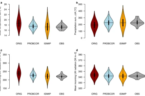
An evaluation of the distribution of variables in the resampled ensemble in Central

Eu-20

rope shows that it not only improves the simulation of seasonal mean temperatures (which it does by construction), but also yields considerable improvements to the simu-lation of rainfall and radiation components (Fig. 3). This suggests that these biases are related to specific synoptic situations in summer, justifying to apply the bias correction approach to summer months. Hence, the multivariate covariance structure between

(17)

ESDD

6, 1999–2042, 2015

S. Sippel et al.

Title Page

Tables Figures

◭ ◮

Back Close

Full Screen / Esc

Discussion

P

a

per

|

Discussion

P

a

per

|

Discussion

P

a

per

|

Discussion

P

a

per

|

temperature, precipitation and radiation as simulated by HadRM3P appears to be well represented in the model simulations posterior to the updating procedure given the reanalysis/observational data. Moreover, while this procedure also improves the sim-ulation of summer temperatures and precipitation on a monthly time scale, virtually no changes in the ensemble statistics are induced to non-summer months (Fig. S1),

5

indicating that the time scales of temporal decorrelation are short enough for a suc-cessful application of the resampling procedure (Fig. S1). However, while conventional statistical bias correction following Hempel et al. (2013) adjusts monthly means of the distributions of precipitation and radiation (by construction), changes are induced by the multiplicative adjustment to the width and shape of the distribution, including its

10

tails (Fig. 3, see also Sect. 4.2).

An evaluation of the resulting spatial patterns of the resampling bias correction shows that the representation of the simulated statistical distributions of temperature and precipitation are considerably improved in Central Europe (area mean constraint) and across the entire European model region (single grid cell constraints, Figs. S2–S3).

15

Remarkably, this holds not only for seasonal averages, but also for higher statistical moments such as the inter-decile range (Figs. S2–S3).

Furthermore, we test the representation of land–atmosphere coupling in the origi-nal and resampled model ensemble by investigating the correlation strength between summer mean temperatures (T) with latent heat (LE) fluxes following Seneviratne et al.

20

(2006). The original HadRM3P ensemble shows strong water limitation of

evapotran-spiration in summer (negative correlation between LE andT) for most temperate and

Mediterranean European regions, thus overestimating soil moisture control compared to reanalysis data and upscaled observations (Fig. S4). In the resampled ensemble, land–atmosphere coupling remains strongly soil moisture controlled in the

Mediter-25

(18)

mem-ESDD

6, 1999–2042, 2015

S. Sippel et al.

Title Page

Tables Figures

◭ ◮

Back Close

Full Screen / Esc

Discussion

P

a

per

|

Discussion

P

a

per

|

Discussion

P

a

per

|

Discussion

P

a

per

|

bers also yields an improved representation of physical processes such as land– atmosphere coupling in the resampled ensemble.

4.2 Sensitivity of climatic extremes to bias correction 4.2.1 Summertime temperature extremes

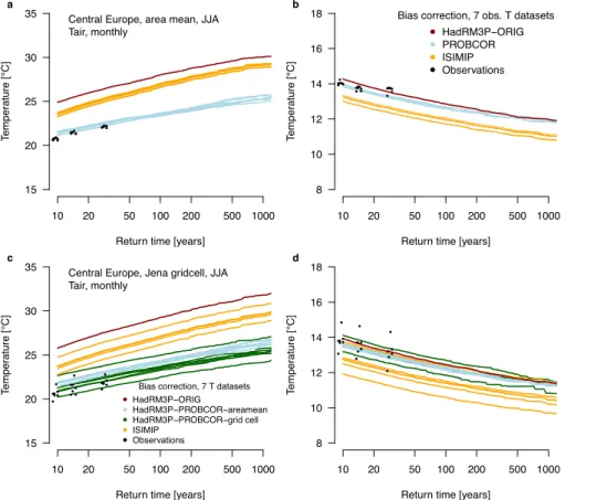
Summertime monthly extreme temperatures are shown in Fig. 4 as a spatial average

5

for the study region located over Central Europe and for an illustrative and randomly chosen grid cell (“Jena grid cell”).

The location, slope and shape of the lines in the return time plots shown in Fig. 4 reveal that the tails of simulated monthly temperature extremes are highly sensitive to the type of bias correction applied, both for a regional average and a single grid cell:

10

Uncorrected simulations overestimate both location and scale (i.e. slope of the line in the return time plot) of positive temperature anomalies in summer, while this is not the case for anomalously cold summer months (Fig. 4). An additive adjustment of monthly means (orange lines in Fig. 4, Hempel et al., 2013) preserves slope and shape of the tail, i.e. preserves the year-to-year variability of simulated monthly temperatures (and

15

biases therein) in the ensemble. Note that this procedure cannot account for the asym-metry between the upper and lower tail of simulated monthly temperatures – i.e. the offset correction leads to an overcorrection of cold months, whereas the statistics of the hot tails improve only marginally. This is confirmed by a statistical extreme value anal-ysis (Figs. S5 and S6): the temperature offset approach adjusts only the location of the

20

GEV yielding spurious artefacts in the (originally well simulated) cold tail, whilst not ac-counting fully for the upper tail due to the aforementioned asymmetries. This is a funda-mental drawback of using linear parametric transfer functions, i.e. even if the variability of the simulated distributions would have been adjusted along with the means (see e.g. Sippel and Otto, 2014), the outlined “asymmetry” issue would not necessarily improve.

25

(19)

ESDD

6, 1999–2042, 2015

S. Sippel et al.

Title Page

Tables Figures

◭ ◮

Back Close

Full Screen / Esc

Discussion

P

a

per

|

Discussion

P

a

per

|

Discussion

P

a

per

|

Discussion

P

a

per

|

as well as on a grid cell constraint yield relatively similar representations of the tails. An evaluation of the extreme value statistics shows that the probabilistic procedure indeed considerably improves the statistical characteristics of the simulated tails in the ensem-ble compared to (long-term) observations (Figs. S5 and S6). To this end, resampling the original ensemble changes location and scale of the extreme value distributions,

5

but the shape parameter of the tails remain effectively unchanged. Some caution is re-quired due to the relatively scarce availability of observed monthly mean temperatures (i.e. 1901–2014), which induces considerable uncertainties to the parameters of the fitted GEV distributions (Figs. S5 and S6). Moreover, the different time periods of ob-servations and ensemble simulations (1986–2011) impede a direct “evaluation” of the

10

bias correction. Nonetheless, this indicative comparison yields very promising results of bias-correcting without invasive changes to the simulated statistical distribution.

Lastly, our analysis shows that any bias correction based on a single grid-cell level in-duces some uncertainty due to the choice of observational dataset. This is an important issue to consider if impact model simulations on a grid cell scale are to be conducted,

15

whereas regional averages are not as strongly affected. Figure 4 shows that resam-pling the ensemble based on a spatial average constraint reduces this uncertainty as compared to adjusting monthly means or resampling on a grid cell scale.

4.2.2 Summertime rainfall extremes

We extend the analysis of the previous paragraph to investigate how resampling based

20

on a temperature constraint alters the representation of summer precipitation in a large ensemble simulation. The original HadRM3P simulated summer seasons are too dry in average over Central Europe (Fig. S2), which is largely due to a much too dry lower tail (Fig. 5), whilst simulated heavy monthly precipitation matches relatively well the available observational data (Fig. 5).

25

(20)

ESDD

6, 1999–2042, 2015

S. Sippel et al.

Title Page

Tables Figures

◭ ◮

Back Close

Full Screen / Esc

Discussion

P

a

per

|

Discussion

P

a

per

|

Discussion

P

a

per

|

Discussion

P

a

per

|

means to match observations (Hempel et al., 2013) leads to an inflation of very wet seasons that are physically implausible given the observations (Fig. 5, orange lines). Likewise, the (biased) dry tail in HadRM3P improves only to a very limited extent if the scaling approach is used. The extreme value analysis (Fig. S6) shows that the multiplicative adjustment changes both location and scale of the tail distribution – and

5

that both parameters are not necessarily improving (indeed often deteriorating, see e.g. scale parameters in Fig. S6 in the Supplement) by applying a simple statistical

bias correction. However, resampling based on atemperature constraint yields a new

ensemble, in which the simulation of both tails has improved (Figs. 5 and S6). Only minor changes have been induced to the (well-simulated) wet tail, whilst the

previ-10

ously strongly biased dry tail has considerably improved (Figs. 5 and S6), indicating that temperature-based resampling as deployed here successfully separates “plausi-ble” ensemble members from the (unrealistic) hot and dry members. The extreme value analysis shows that resampling largely alters the location of the simulated distribution of seasonal rainfall extremes, whilst the scale and shape of the tails remain largely

15

unchanged.

To conclude, it was shown that resampling based on a univariate observations-based temperature constraint improves the simulation of rainfall variability and extremes by teasing out ensemble members that are implausibly hot and dry in our case study region.

20

4.3 The impact of bias correction on simulated ecosystem water and carbon fluxes

In this subsection, we present HadRM3P-LPJmL ensembles of simulated fluxes of car-bon and water and discuss bias correction methods with a focus on the extreme tails of the simulated distributions. Further, we investigate the sensitivity of the simulated

25

carbon fluxes to an accurate representation of rainfall in the climatic input data.

(21)

ESDD

6, 1999–2042, 2015

S. Sippel et al.

Title Page

Tables Figures

◭ ◮

Back Close

Full Screen / Esc

Discussion

P

a

per

|

Discussion

P

a

per

|

Discussion

P

a

per

|

Discussion

P

a

per

|

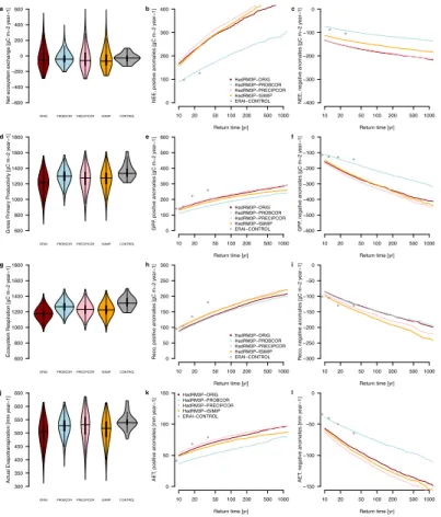
simulation. Conventional statistical bias correction that matches monthly means of the

HadRM3P ensemble exactly to those of the ERA-Interim control climate simulation

yields differences in fluxes of−6.6,−7.5 and −4.7 % for GPP, Reco and AET, respec-tively. Note that differences in the resampled HadRM3P ensemble are less pronounced (−4.2, −4.5, and−2.0 %, respectively), although no attempt has been made to adjust

5

the statistical properties of the model output. Those differences in simlated annual mean fluxes are related to higher statistical moments of the statistical distributions and shown in Fig. 6.

To this end, simulated GPP, NEE, and AET show strong asymmetry in their simulated distributions (Fig. 6): negative anomalies in GPP and AET are much more pronounced

10

than positive ones; this holds also for NEE but with an inverted sign (ecosystem carbon release corresponds to positive fluxes). However, the simulation of these extremes is highly sensitive to bias correction, where the lower tails of GPP and AET in the original and statistically bias corrected ensemble strongly overestimate reductions in carbon and water flux. In contrast, negative GPP and AET anomalies in the resampled

15

ensemble (corresponding to positive ones in NEE) exhibit a much less pronounced lower tail and asymmetry and agree well with the control simulations.

For example, a positive anomaly in NEE corresponding to a 30 year return period ex-ceeds+200 g C m−2_a−1 _{in the conventionally bias corrected simulations and the}

orig-inal ensemble, whereas such an anomaly in the resampled ensemble hardly reaches

20

+150 g C m−2_a−1 _{(Fig. 6b) roughly corresponding to an empirical 30 year return event}

in the ERA-Interim control simulations. Similar arguments can be made for negative anomalies in annual GPP and annual AET (Fig. 6). The di_fferent tails of the simulations occur because the original meteorological ensemble implies large hot and dry biases in summer, inducing negative anomalies in ecosystem–atmosphere carbon and water

25

(22)

PRE-ESDD

6, 1999–2042, 2015

S. Sippel et al.

Title Page

Tables Figures

◭ ◮

Back Close

Full Screen / Esc

Discussion

P

a

per

|

Discussion

P

a

per

|

Discussion

P

a

per

|

Discussion

P

a

per

|

CIPCOR and ISIMIP are identical to the control climate simulation, which highlights the importance to consider statistical moments beyond the mean for impact simulations.

However, note that the positive tails of GPP and AET are not as strongly affected. Furthermore, ecosystem respiratory fluxes show a relatively lower sensitivity to bias correction (i.e. to hot and dry summer conditions).

5

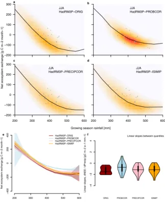
Further, we investigate whether different bias correction schemes induce different sensitivities of LPJmL simulated carbon fluxes to rainfall. Here, the relationship be-tween a growing season rainfall proxy (April–September rainfall sums) and annual NEE is characterized using piecewise linear regression (Fig. 7a–d). Figure 7e shows that LPJmL simulated annual NEE responds to rainfall in a roughly similar way across

dif-10

ferent bias correction schemes, which highlights the need of an accurate representation of precipitation in climate impact simulations in the terrestrial biosphere. However, char-acterizing the annual NEE response for each quantile of the rainfall distribution shows that the resampled rainfall distribution (PROBCOR) leads to a less negative NEE re-sponse to rainfall (larger slopes in Fig. 7f), whereas a dry summer tail (in the ORIG,

15

ISIMIP, and PRECIPCOR simulations) yields a generally stronger NEE response (more negative sloped in Fig. 7f).

In conclusion, different bias correction methods induce different statistical properties of simulated ecosystem–atmosphere fluxes of carbon and water. This affects the vari-ability and skewness of NEE, GPP and AET simulations (as shown in Fig. 6), where hot

20

and dry biases in summer imply a disproportional reduction in carbon and water fluxes in climatically “unfavourable” years. Conventional statistical bias correction cannot ac-count for this issue, whereas the novel probabilistic bias correction schemes alleviates those biases to a very large extent.

5 Discussion

25

(23)

ESDD

6, 1999–2042, 2015

S. Sippel et al.

Title Page

Tables Figures

◭ ◮

Back Close

Full Screen / Esc

Discussion

P

a

per

|

Discussion

P

a

per

|

Discussion

P

a

per

|

Discussion

P

a

per

|

regional climate model output. The methodology is conceptually similar to earlier ap-proaches designed to constrain future probabilistic climate predictions based on obser-vational constraints (Piani et al., 2005; Collins, 2007). Its application has been shown in this paper to yield considerably improved simulations of weather and climate extremes. Remarkably, the improvement holds for variables that have not been constrained upon

5

(i.e. constraining on seasonal mean temperatures improves the representation of mean and extreme precipitation), which indeed emphasizes the importance to bias correct in a physically meaningful way. Furthermore, simple but widely used statistical bias cor-rection methodologies (e.g. Hempel et al., 2013) have been evaluated with respect

to the effect on the representation of weather and climate extremes on monthly to

10

seasonal time scales. These methods cannot account for biases associated with e.g. specific synoptic situations that result in biases in higher statistical moments of the simulated distributions, which indeed emphasizes the importance to bias correct in a physically meaningful way. We demonstrated that this shortcoming of conventional methodologies can be detrimental to statistics of weather and climate extremes and

15

their variability. Although more sophisticated statistical bias-correction schemes (see Gudmundsson et al. (2012) for an overview) might have an improved skill in rectifying biases in higher statistical moments (such as e.g. asymmetries in simulated distribu-tions) have not been explicitly tested in this study, the fundamental question of how physical consistency can be preserved after bias correction (Ehret et al., 2012),

in-20

cluding multivariate dependencies between variables, remains elusive. Therefore non-linear and nonparametric bias correction techniques (Gudmundsson et al., 2012) might potentially improve statistics of extreme events if a large enough sample of observa-tions is available, but cannot retain physical consistency (Sippel and Otto, 2014) and may ultimately fall short for correcting a set of input variables.

25

(24)

ESDD

6, 1999–2042, 2015

S. Sippel et al.

Title Page

Tables Figures

◭ ◮

Back Close

Full Screen / Esc

Discussion

P

a

per

|

Discussion

P

a

per

|

Discussion

P

a

per

|

Discussion

P

a

per

|

water fluxes (Sect. 4.3). Mechanistically, the stark contrast between the bias correction schemes can be traced back to the sensitivity of the LPJmL model to dry conditions (see e.g. Rammig et al., 2015; Rolinski et al., 2015): NEE, GPP and AET in Central Europe are to a large extent driven by the availability of rainfall in the growing season, except for wet conditions, under which the relationship levels off(Fig. 7). Bias correction

5

strongly affects the variability and extremes of rainfall (as shown above), thus inducing pronounced asymmetries in simulated water and carbon fluxes (Figs. 7f and 6). There-fore, our results highlight the importance to account not only for biases in the mean but also for higher moments in the climatic input in order to generate robust insights into the past, present and future climate impacts. Our results demonstrate that physically

10

consistent bias correction schemes might be preferable for this task. Moreover, it has been shown recently that climatic drivers exert multivariate controls on ecosystem re-sponses such as phenology and vegetation greenness dynamics (Forkel et al., 2015), therefore accurate ecosystem impact simulations requires bias correction schemes that preserve the correlation structure of climatic data.

15

However, several limitations of the present methodology should be discussed: First, probabilistic resampling based on a regional observational constraint cannot account for biases on very large regional or continental scales if the biases show a spatially or temporally heterogenous structure or gradients. In the latter case, resampling-based bias correction could lead to spurious artefacts in the spatio-temporal structure of the

20

bias-corrected model domain. Secondly, a careful evaluation of the ensemble resam-pling approach has to be made – particularly with a focus on the spatial and temporal extent of the constraint and the resampled ensemble: A trade-o_ff exists between re-sampling on small domains (e.g. grid-cell based) that is sensitive to the choice of ob-servational dataset, and very large domains that might be prone to a spatio-temporal

25

(25)

sim-ESDD

6, 1999–2042, 2015

S. Sippel et al.

Title Page

Tables Figures

◭ ◮

Back Close

Full Screen / Esc

Discussion

P

a

per

|

Discussion

P

a

per

|

Discussion

P

a

per

|

Discussion

P

a

per

|

ilarly to the current practice of statistical bias correction (e.g. Hempel et al., 2013) would be straightforward, i.e. based on a calibration using present or past conditions. Lastly, the resampling approach requires relatively large ensemble sizes to be effective: in order to plausibly cover the climate space in any particular location, the simulated ensemble should cover the entire observed distribution. However, this condition does

5

not necessarily restrict resambling-based bias correction methods to large ensembles simulations: For example, under the assumption of ergodicity for a given time period, resampling shorter time periods (e.g. single years) from smaller ensembles such as CORDEX regional simulations (Giorgi et al., 2009) would provide a promising topic for further study.

10

Notwithstanding these limitations however, we show the usefulness of the novel bias correction scheme that might be a useful and physically consistent alternative to con-ventional statistical bias correction as long as global and regional dynamical climate models su_ffer from pertinent biases.

6 Conclusions

15

In this paper, we introduced a novel bias correction method that retains physical consis-tency and the multivariate correlation structure of the climate model output based on an ensemble resampling approach. We showed that such an approach strongly improves

a. statistics of weather and climate extreme events, and

b. the simulation of climate impacts such as ecosystem–atmosphere fluxes of

car-20

bon and water, including extremes and variability therein.

The methodology could be readily taken up in probabilistic event attribution studies that deploy large ensembles simulations (see Stott et al. (2013) for an overview) in order to more realistically describe the statistics of (changing) extreme events.

Furthermore, detecting and attributing the impacts of climatic variability and

ex-25

(26)

ESDD

6, 1999–2042, 2015

S. Sippel et al.

Title Page

Tables Figures

◭ ◮

Back Close

Full Screen / Esc

Discussion

P

a

per

|

Discussion

P

a

per

|

Discussion

P

a

per

|

Discussion

P

a

per

|

research area (Stone et al., 2009, 2013), including demonstrated interest by stake-holders across various sectors (Schiermeier, 2011; Stott and Walton, 2013; Sippel et al.b)Sippel, Walton). To this end, our study showed that it is crucial to account for higher statistical moments in biased climatic input data, and to correct climatic biases in a physically consistent way. Therefore, our methodology could be taken up by the

5

climate impact modelling community to reduce climate forcing biases to a very large extent without requiring any modifications to the climate model output.

The Supplement related to this article is available online at doi:10.5194/esdd-6-1999-2015-supplement.

Acknowledgements. We would like to thank our colleagues at the Oxford eResearch Centre for

10

their technical expertise, the Met Office Hadley Centre PRECIS team for their technical and sci-entific support for the development and application of weather@home and all of the volunteers who have donated their computing time to climateprediction.net. We thank Richard Jones, An-tje Weisheimer, Lukas Gudmundsson, Jose Manuel Gutierrez Llorente, Nuno Carvalhais, Mirco Migliavacca and Soenke Zaehle for comments and productive discussions regarding the bias

15

correction of regional climate model output.

We appreciate the creators and providers of observational and reanalysis datasets, includ-ing in particular the Berkeley Earth Observations (Rohde et al., 2013), University of East Anglia Climatic Research Unit (CRU, TS3.2, Phil Jones and others; Harris et al., 2014), CRUNCEP dataset (http://dods.extra.cea.fr/data/p529viov/cruncep/readme.htm), Global

Pre-20

cipitation Climatology Centre (GPCC) Full Data Reanalysis Version 6.0 at Deutscher Wet-terdienst (Schneider et al., 2011, 2014), the E-OBS dataset from the EU-FP6 project EN-SEMBLES (http://ensembles-eu.meto_ffice.com) and the data providers in the ECA&D project (http://www.ecad.eu), ERA-Interim data provided courtesy ECMWF, and the WATCH-Forcing-Data-ERA-Interim (WFDEI).

25

(27)

ESDD

6, 1999–2042, 2015

S. Sippel et al.

Title Page

Tables Figures

◭ ◮

Back Close

Full Screen / Esc

Discussion

P

a

per

|

Discussion

P

a

per

|

Discussion

P

a

per

|

Discussion

P

a

per

|

References

Allen, M.: Liability for climate change, Nature, 421, 891–892, 2003. 2001

Barriopedro, D., Fischer, E. M., Luterbacher, J., Trigo, R. M., and Garc’ia-Herrera, R.: The hot summer of 2010: redrawing the temperature record map of Europe, Science, 332, 220–224, 2011. 2001

5

Beer, C., Weber, U., Tomelleri, E., Carvalhais, N., Mahecha, M., and Reichstein, M.: Harmo-nized European long-term climate data for assessing the effect of changing temporal vari-ability on land–atmosphere CO₂fluxes, J. Climate, 27, 4815–4834, 2014. 2034

Bellprat, O., Kotlarski, S., Lüthi, D., and Schär, C.: Physical constraints for temperature biases in climate models, Geophys. Res. Lett., 40, 4042–4047, 2013. 2003

10

Bindoff, N. L., Stott, P. A., AchutaRao, M., Allen, M. R., Gillett, N., Gutzler, D., Hansingo, K., Hegerl, G., Hu, Y., Jain, S., Mokhov, I. I., Overland, J., Perlwitz, J., Sebbari, R., and Zhang, X.: Detection and attribution of climate change: from global to regional, in: Climate Change 2013, The Physical Science Basis, Contribution of Working Group I to the Fifth Assessment Report of the Intergovernmental Panel on Climate Change, Cambridge University Press, Cambridge,

15

UK, New York, NY, USA, 2013. 2001

Boberg, F. and Christensen, J. H.: Overestimation of Mediterranean summer temperature pro-jections due to model deficiencies, Nat. Clim. Change, 2, 433–436, 2012. 2006

Bondeau, A., Smith, P. C., Zaehle, S., Schaphoff, S., Lucht, W., Cramer, W., Gerten, D., Lotze-Campen, H., Müller, C., Reichstein, M., and Smith, B.: Modelling the role of agriculture for

20

the 20th century global terrestrial carbon balance, Global Change Biol., 13, 679–706, 2007. 2006, 2007

Buser, C. M., Künsch, H., Lüthi, D., Wild, M., and Schär, C.: Bayesian multi-model projection of climate: bias assumptions and interannual variability, Clim. Dynam., 33, 849–868, 2009. 2003, 2006

25

Chapin III, F. S., Woodwell, G. M., Randerson, J. T., Rastetter, E. B., Lovett, G. M., Baldoc-chi, D. D., Clark, D. A., Harmon, M. E., Schimel, D. S., Valentini, R., Wirth, C., Aber, J. D., Cole, J. J., Goulden, M. L., Harden, J. W., Heimann, M., Howarth, R. W., Matson, P. A., McGuire, A. D., Melillo, J. M., Mooney, H. A., Neff, J. C., Houghton, R. A., Pace, M. L., Ryan, M. G., Running, S. W., Sala, O. E., Schlesinger, W. H., and Schulze, E.-D.: Reconciling

30

(28)

ESDD

6, 1999–2042, 2015

S. Sippel et al.

Title Page

Tables Figures

◭ ◮

Back Close

Full Screen / Esc

Discussion

P

a

per

|

Discussion

P

a

per

|

Discussion

P

a

per

|

Discussion

P

a

per

|

Christensen, J. H., Boberg, F., Christensen, O. B., and Lucas-Picher, P.: On the need for bias correction of regional climate change projections of temperature and precipitation, Geophys. Res. Lett., 35, L20709, doi:10.1029/2008GL035694, 2008. 2003

Christensen, J. H., Kjellström, E., Giorgi, F., Lenderink, G., and Rummukainen, M.: Weight assignment in regional climate models, Clim. Res., 44, 179–194, 2010. 2013

5

Ciais, P., Reichstein, M., Viovy, N., Granier, A., Ogée, J., Allard, V., Aubinet, M., Buchmann, N., Bernhofer, C., Carrara, A., Chevallier, F., De Noblet, N., Friend, A. D., Friedlingstein, P., Grün-wald, T., Heinesch, B., Keronen, P., Knohl, A., Krinner, G., Loustau, D., Manca, G., Matteucci, G., Miglietta, F., Ourcival, J. M., Papale, D., Pilegaard, K., Rambal, S., Seufert, G., Soussana, J. F., Sanz, M. J., Schulze, E.-D., Vesala, T., and Valentini, R.: Europe-wide reduction in

pri-10

mary productivity caused by the heat and drought in 2003, Nature, 437, 529–533, 2005. 2001

Coles, S., Bawa, J., Trenner, L., and Dorazio, P.: An Introduction to Statistical Modeling of Extreme Values, vol. 208, Springer, London, 2001. 2013

Collins, M.: Ensembles and probabilities: a new era in the prediction of climate change, Philos.

15

T. Roy. Soc. A, 365, 1957–1970, 2007. 2013, 2021

Dee, D., Uppala, S., Simmons, A., Berrisford, P., Poli, P., Kobayashi, S., Andrae, U., Bal-maseda, M., Balsamo, G., Bauer, P., Bechtold, P., Beljaars, A. C. M., van de Berg, L., Bidlot, J., Bormann, N., Delsol, C., Dragani, R., Fuentes, M., Geer, A. J., Haimberger, L., Healy, S. B., Hersbach, H., Holm, E. V., Isaksen, L., Kallberg, P., Kohler, M., Matricardi, M., McNally, A.

20

P., Monge-Sanz, B. M., Morcrette, J. J., Park, B. K., Peubey, C., de Rosnay, P., Tavolato, C., Thepaut, J. N., and Vitart, F.: The ERA-Interim reanalysis: Configuration and performance of the data assimilation system, Q. J. Roy. Meteorol. Soc., 137, 553–597, 2011. 2006, 2008, 2034

Donat, M., Alexander, L., Yang, H., Durre, I., Vose, R., Dunn, R., Willett, K., Aguilar, E.,

25

Brunet, M., Caesar, J., Hewitson, B., Jack, C., Tank, A. M. G. K., Kruger, A. C., Marengo, J., Peterson, T. C., Renom, M., Rojas, C. O., Rusticucci, M., Salinger, J., Elrayah, A. S., Sekele, S. S., Srivastava, A. K., Trewin, B., Villarroel, C., Vincent, L. A., Zhai, P., Zhang, X., and Kitching, S.: Updated analyses of temperature and precipitation extreme indices since the beginning of the twentieth century: the HadEX2 dataset, J. Geophys. Res.-Atmos., 118,

30

2098–2118, 2013. 2001