www.hydrol-earth-syst-sci.net/19/4641/2015/ doi:10.5194/hess-19-4641-2015
© Author(s) 2015. CC Attribution 3.0 License.
Novel indices for the comparison of precipitation extremes
and floods: an example from the Czech territory
M. Müller1,2, M. Kašpar1, A. Valeriánová3, L. Crhová3, E. Holtanová3, and B. Gvoždíková2
1Institute of Atmospheric Physics AS CR, Prague, Czech Republic 2Faculty of Science, Charles University, Prague, Czech Republic 3Czech Hydrometeorological Institute, Prague, Czech Republic
Correspondence to:M. Müller ([email protected])
Received: 2 December 2014 – Published in Hydrol. Earth Syst. Sci. Discuss.: 9 January 2015 Revised: 3 November 2015 – Accepted: 5 November 2015 – Published: 24 November 2015
Abstract. This paper presents three indices for evaluation
of hydrometeorological extremes, considering them as areal precipitation events and trans-basin floods. In contrast to common precipitation indices, the weather extremity index (WEI) reflects not only the highest precipitation amounts at individual gauges but also the rarity of the amounts, the size of the affected area, and the duration of the event. Further-more, the aspect of precipitation seasonality was considered when defining the weather abnormality index (WAI), which enables the detection of precipitation extremes throughout the year. The precipitation indices are complemented with the flood extremity index (FEI) employing peak discharge data. A unified design of the three indices, based on return periods of station data, enables one to compare easily inter-annual and seasonal distributions of precipitation extremes and large floods.
The indices were employed in evaluation of 50 hydrom-eteorological extremes of each type (extreme precipitation events, seasonally abnormal precipitation events, and large floods) during the period 1961–2010 in the Czech Repub-lic. A preliminary study of discrepancies among historic val-ues of the indices indicated that variations in the frequency and/or magnitude of floods can generally be due not only to variations in the magnitude of precipitation events but also to variations in their seasonal distribution and other factors, primarily the antecedent saturation.
1 Introduction
Precipitation is extensively studied due to its impacts on the hydrology, geomorphology, and economy of a given region. Precipitation extremes are of special interest because impacts rapidly increase with the precipitation extremity. There are three main concepts of extremity: severity, intensity, and rar-ity (Stephenson, 2008). Evaluation of the extremrar-ity of past events enables one to determine return periods of heavy pre-cipitation and to estimate the probable maximum precipita-tion ( ˇRezáˇcová et al., 2005b). Currently, the main challenge in precipitation climatology is understanding past and pos-sible future changes in the frequency and/or magnitude of precipitation extremes (e.g., Alexander et al., 2006). These changes could alter the frequency and/or magnitude of conse-quent floods. To properly assess this linkage, we need to de-fine quantitative indices to investigate the coupling between precipitation extremes and flood events.
The concept of intensity better corresponds to physical causes; thus, it is more convenient for comparison between precipitation extremes and floods. Rodier and Roche (1984) and lately Herschy (2003) assessed the world’s maximum floods with respect to their maximum instantaneous dis-charges. To compare the extremity of floods on various rivers, they used the Francou index, which normalizes the common logarithm of maximum discharge by the common logarithm of the catchment area. Not surprisingly, maximum floods were located in the rainiest regions.
The standard approach to the evaluation of precipitation intensity is to search data series from individual gauges us-ing commonly accepted indices (Zhang et al., 2011), mainly those defined by the Expert Team on Climate Change Detec-tion and Indices (ETCCDI). According to ETCCDI, precipi-tation extremes can be defined as days with maximum 1-day (P1) or 5-day (P5) precipitation total in a period.
Neverthe-less, the duration of events can vary widely, and the precip-itation intensity usually fluctuates during the event. Begue-ria et al. (2009) partly took account of this fact; they used declustering of daily precipitation totals to distinguish indi-vidual precipitation events and characterized them not only by magnitude and duration but also by peak intensity.
Even more important is the spatial aspect of precipitation events. They always affect a certain area; thus, precipitation extremes should be considered to be “regional events” (Ren et al., 2012). The latter approach is necessary if the inten-sity of precipitation and floods is to be compared, because the size of the affected area influences the hydrological re-sponse. In our previous paper (Kašpar and Müller, 2008), we used the concept of areal precipitation intensity and evalu-ated precipitation events based on the weighted average of daily areal precipitation totals on 3 consecutive days. Never-theless, Konrad (2001) demonstrated that the extremity of an event depends on the size of the considered region. As a re-sult, the areal average disadvantages events that were violent but affected only a part of the region over which the mean is taken (e.g., an administrative unit, a catchment).
Based on the concept of intensity, extreme events occur mainly in regions that are prone to heavy rains (in the Czech Republic, such regions are along the northern state border be-cause of the orographic precipitation enhancement). In order to reflect regional climatic differences, the concept of rarity is applied; extreme precipitation and floods can thus be de-tected in the whole studied region. The concept is frequently used with regard to floods, and the intensity (magnitude of the peak flow) is usually compared with return levels. If a set of extreme floods is studied, they are defined as discharges with return periods exceeding a threshold. Nevertheless, Uh-lemann et al. (2010) noted that flood events frequently affect several independent catchments and introduced the concept of trans-basin floods. We adopted and adapted this approach to our data because we compared flood extremity with pre-cipitation, which also affects more than one catchment at a given time.
Table 1.Acronyms for proposed indices and studied
hydrometeo-rological extremes.
WEI Weather extremity index
WAI Weather abnormality index
FEI Flood extremity index
EPE Extreme precipitation event
APE (Seasonally) abnormal precipitation event
EFE Extreme flood event
To enable this comparison, we propose indices that are based on the point estimates of return periods of precipitation totals and peak discharges and on spatial averaging of the val-ues (Sects. 2.1, 2.3). The method is further enriched by the aspect of precipitation abnormality with respect to the season (Sect. 2.2). We demonstrate the method using data from the Czech Republic and present three sets of events: precipitation extremes regardless of and regarding the season and extreme floods (Sect. 3.1). These sets are further compared with re-gard to their inter-annual (Sect. 3.2) and seasonal (Sect. 3.3) distribution. The results obtained are discussed in Sect. 4.
2 Proposed methods
We proposed three extremity indices that enable one to com-pare the temporal distribution of precipitation extremes and floods. The indices are based on point return period estimates of precipitation totals and peak flows, respectively, spatial averaging of their values, and optimizing the areal extent and the duration of individual events. Table 1 summarizes acronyms for proposed indices and studied hydrometeoro-logical extremes.
2.1 Evaluation of precipitation extremity
0 20 40 60 80 100 120 140
10 100 1000 10000 100000
Eta
,
WE
I
a [km2]
t=5 (30/5-3/6) t=4 (30/5-2/6) t=3 (1-3/6) t=2 (1-2/6) t=1 (1/6)
WEI = 123 (5d)
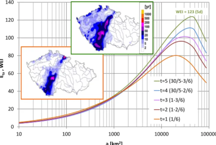
Figure 1.Determination of the WEI of the EPE in May–June 2013
by maximizingEt a. The inset maps present interpolated return
pe-riods of 1-day totals on 1 June (left) and of 5-day totals from 30 May to 3 June (right).
of the ROI method makes the estimations more robust than local analyses (Kyselý et al., 2011), we did not accept return periods longer than 1000 years. Instead, we set the return pe-riod to 1000 years.
The next step in the method is the interpolation of re-turn periods from gauges in a regular grid. Experiments have demonstrated that the results are not affected by the resolu-tion if it is constant across all studied events; we used a hor-izontal resolution of 2 km in the presented study. Because of the exponential nature of the GEV distribution from which the return periods are derived, common logarithms of the return period are interpolated instead of pure return period values. We chose linear kriging as the interpolation method. Using an inversion transformation, cell values ofNt iare
ob-tained; the value represents the return period of the precipita-tion total accumulated duringt days in a celli. The cells are
then sorted in decreasing order with respect toNt iand
con-sidered within a stepwise increasing areaaofnpixels (each
representing 4 km2for the chosen horizontal resolution). The WEI is calculated by maximizing the variable Et a.
This variable is defined as the common logarithm of the spa-tial geometric meanGt aof the return periodsNt imultiplied
by the radiusRof a circle of the same area as the one over
which the geometric mean is taken. This relationship can be expressed as
Et a=log(Gt a) R=
n
P
i=1
log(Nt i)
n
√a
√π. (1)
The optimization ofais performed using a step-by-step
en-larging of the area under consideration. The variableEt a
ini-tially increases as we accumulate cells with lengthy return periods; once the return periods are insufficiently long in the added cells, the value ofEt astarts to decrease. When
choos-0 5 10 15 20 25 30 35 40 45 50
0 20 40 60 80 100 120 140 160 180 200
4/8 5/8 6/8 7/8 8/8 9/8 10/8 11/8 12/8 13/8
Pmea
n
[mm
]
Eta
, WEI
Pmean [mm]
Eta 1d
Eta 2d
Eta 3d
Eta 4d
Eta 5d
(Eta 7d)
WEI = 104 (2d)
WEI = 174 (3d)
Figure 2.Mean daily precipitation totalsPmeanin the Czech
Re-public (right axis) and respective maximum values ofEt aon 4–13
August 2002 (color bars, left axis). Selected maximumEt avalues
for time windows with various lengths oftdays are depicted
includ-ing the hypothetical value of maximumEt afor the 7-day period of
6–12 August.
ing a time window for whichEt areaches its maximum
dur-ing the entire event, the respective maximumEt aequals the
WEI. Then, it is also possible to determine the affected area
a, the durationt, and the respective geometric mean of return
periods Gt a complying with the relationship Et a=WEI.
The method is presented in Fig. 1, which shows the EPE from May–June 2013, which was subsequently added to the study because of catastrophic flooding observed during this time (Šercl et al., 2013). Although the maximum return pe-riod at a site belonged to the 1-day total on 1 June (Horní Maršov, 130.3 mm,>1000 years), maximumEt a gradually
increased with increasingt. The WEI corresponded to the
5-day period from 30 May to 3 June 2013.
Nevertheless, the time distribution of maximumEt a
val-ues can be more complex. Figure 2 presents such a case from August 2002, when a subsequent EPE followed the previ-ous one after a break of only 3 days. In this case, two dis-tinct maxima of Et a enabled us to recognize independent
EPEs and determine the durations of both events (2 and 3 days, respectively). Adding an extra day would cause theEt a
value to decrease. Therefore, we did not consider a longer time window (7 days); still theEt awould be even higher as
the two EPEs would be aggregated. Moreover, we also de-cided to consider precipitation events of the length from 1 to 5 days only because the thresholds correspond with two main indices of precipitation extremes by ETCCDI (Zhang et al., 2011).
Figure 2 also shows that the extremity of precipitation with respect to the maximumEt acan substantially differ from the
concept ofEt ais that the considered area and the time
win-dow are event-adjusted. Although comparably heavy rains were limited to southwestern Czech Republic on both days, weaker rains occurred only on the latter day throughout the whole country. These non-extreme precipitation totals gener-ally increase the mean, whereas they are not included in the
Et a.
2.2 Precipitation abnormality with respect to the
season
Both precipitation long-term means and extremes are not equally distributed among the seasons in most places on the Earth. In the Czech Republic, higher precipitation totals gen-erally occur in summer (Tolasz et al., 2007). As a result, the WEI maxima are also concentrated in the summer.
However, even smaller precipitation totals can be consid-ered to be extreme when they occur in a season when they are rare. If precipitation extremes are defined as events sig-nificantly different from seasonally normal conditions, then they can occur throughout the year. Precipitation extremes of this type will be referred to as abnormal precipitation events (APEs). They were evaluated using the weather abnormity index (WAI), which has the same design as the WEI, al-though it is calculated based on seasonally standardized pre-cipitation totals.
The standardization of daily precipitation totals reflects their annual distribution. The mean, variance and skewness fluctuate significantly during the year (Fig. 3), and thus none of these parameters can be avoided in the process of stan-dardization. The same is true for the kurtosis, which is very closely correlated with the skewness (not depicted). Further-more, means and standard deviations are also closely cor-related. Therefore, our standardization method consists of removing fluctuations of the meanµdand the skewnessγd
from the daily totals on individual calendar daysd.
There are two types of fluctuations in the data. First,µd andγd change significantly from day to day depending on the presence or absence of heavy precipitation episodes on a given calendar day. These random fluctuations have to be smoothed using a proper time filter. Monthly means are sometimes used for these purposes, but we have excluded this method as it produces artificial edges in the data. Mov-ing averages are only slightly better from this point of view. We used the Gaussian filter because it is considered the ideal time domain filter (Blinchikoff and Zverev, 2001). We tested several data series to identify the most appropriate length of the filter and chose Gaussian smoothing with a standard devi-ationσof 30 days and a time window of 3σ. Time-smoothed
values of the mean and skewness are hereinafter referred to asµdGandγdG, respectively.
Even the values ofµdGandγdGfluctuate through the year because of seasonal changes in precipitation climatology. The actual daily totals P1 are standardized using the rela-tionship
0 1 2 3 4 5 6
0 5 10 15 20 25 30
1/1 1/4 1/7 1/10 31/12
Sk
e
wness
Mean,
st
andar
d
de
via
tion
Calendar days
mean stdev mean_sm stdev_sm skew skew_sm
Figure 3.Annual cycle of the mean, standard deviation, and
skew-ness of daily precipitation totals at Churáˇnov station. Individual points represent the values of the mean, standard deviation, and skewness calculated for each calendar day taking into account the period of 1961–2010; curves depict data smoothed using the Gaus-sian filter.
Pms=P
P1
µdG
γγ
dG
, (2)
wherePms is the seasonally standardized daily total,µdGis the time-smoothed mean, γdG is the time-smoothed skew-ness of the distribution of daily totals≥0.1 mm for a calen-dar dayd, andP =E (µdG)andγ=E (γdG). The
transfor-mation (Eq. 2) directly standardizes the mean and skewness and indirectly standardizes the standard deviation and kurto-sis of the daily data. The correction usingP andγ induces
an important feature of seasonally standardized daily totals: their mean annual sum equals the actual mean annual total. This process only redistributes precipitation amounts within the data series: seasonally standardized daily totals become higher and lower in seasons that are less and more exposed to high precipitation, respectively.
0 20 40 60 80 100 120 140
1/1 1/4 1/7 1/10 31/12
Pr
ecipit
a
tion
tot
al
[
mm
]
P1 Pm Pms
28/10/1998 31/7/1977
19/7/1981
11/8/2002 12/8/2002
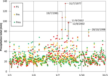
Figure 4.Daily precipitation maxima on individual calendar days
at Churáˇnov station during the 1961–2010 period: non-standardized
totals (P1), totals standardized for the mean and variance only
(Pm=P Pd/µdG)and fully standardized totals (Pms). Dates of
sig-nificant totals are indicated (day/month/yr).
2.3 Evaluation of flood extremity
To compare the precipitation and flood extremity, we also designed the flood extremity index (FEI), which is analo-gous to the WEI and enables us to recognize extreme flood events (EFEs). The FEI is based on return periods of peak discharges at individual sites. In the presented study, we used data from 198 Czech gauges beginning in 1961. However, only the approximate return period values ofN=5, 10, 20,
50, or 100 years were available. Each site represents a catch-ment with an area exceeding 100 km2. If there are one or more considered sites upstream, the catchment area does not include the respective sub-catchments.
By analogy to the WEI, we combine the extremity at each site j expressed by the return period Nj with the area of
the respective catchmentaj. The area of the basin indirectly
represents the magnitude of the river. Return periods were considered without evaluating the possible human impact on peak discharge so the value of the FEI represents the actual course of the flood instead of the theoretical one. Neverthe-less, the very high discharges that are crucial for the evalua-tion of an event are generally less affected by human activi-ties (Langhammer, 2008).
The FEI is defined as the maximum of the variable Fa,
which is given by the equation
Fa=
h
P
j=1
log(Nt i) aj
aa
√a
a
√π. (3)
The aggregated areaaaconsists ofh=1, . . .,198 considered
catchments, which are ordered according toNj in
descend-ing order. Return periods shorter than 5 years are assigned
a value ofNj=1, so that log(Nj)=0 and the respective
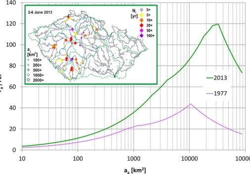
catchments do not contribute to the resultant FEI value. The method is demonstrated in Fig. 5, which compares flooding in the Czech territory due to the EPEs in August 1977 and in May–June 2013. TheFacurve representing the
2013 EFE increases more rapidly and starts to decrease later than in 1977; maxima of the curves depict values of the FEI. The reason is that return periods of peak discharges did not reach 50 years during the first event, whereas during the latter event, the total area of catchments corresponding to gauges with peak flows ofNj≥100 years exceeded 2000 km2, and
the value ofaacorresponding to the FEI was larger. Unlike in Fig. 1, the curves are not fluent because only discrete values ofNj were used (see above).
Because of similarities between Eqs. (1) and (3), the WEI and the FEI reach values of the same order. Nevertheless, val-ues of the FEI were usually slightly smaller in the presented study for several reasons, primarily because all return periods between two values (20 and 50 years, for example) were as-signed the lower value. Moreover, the maximum values were 100 and 1000 years when calculating the FEI and the WEI, respectively.
A serious problem is the separation of individual EFEs if additional peaks occur during a short period in the same catchments. We decided to separate EFEs with respect to EPEs. For example, we distinguished two EFEs in August 2002 because they were produced by two independent EPEs (Fig. 2). Naturally, the extremity of the latter EFE was af-fected not only by the latter EPE but also by the previous one in such a case; this fact can partly explain the discrepan-cies between the extremity of precipitation and of subsequent flooding.
Finally, we tried to assess how much the FEI can be in-fluenced by human regulations. Therefore, a parallel calcu-lation of the FEI was performed (hereinafter FEI_97) using only data from 97 Czech stations where no reservoir with flood protection function is present upstream. A linear de-pendence was detected between the FEI and the FEI_97 with Pearson correlation coefficient as high as 0.86. For example, four maximum EFEs were evaluated as the extremes regard-less either the FEI or the FEI_97 is used. Only four outliers were detected when the FEI_97 was substantially reduced; it happened because flooding occurred almost only in catch-ments not involved in the FEI_97 calculation. Nevertheless, since the FEI_97 represents only rather small catchments, we prefer to use the FEI, which seems to be robust enough also from the viewpoint of human regulations.
2.4 Comparison of precipitation extremes and floods
0 20 40 60 80 100 120 140
10 100 1000 10000 100000
Fa
, F
EI
aa [km2]
2013
1977
Figure 5.Evaluation of extremity of floods in May–June 2013 and in August 1977 using the FEI. The step-by-step aggregated catchments
are ordered in descending order with respect to return periods recorded there. The inset map presents return periodsNjof peak discharges
at gauges in 2013; blue and green curves correspond to the main rivers and watersheds, respectively.
Ce=100WEIFEI (4)
and
Ca=100WAIFEI. (5)
Values significantly above and below average resulting from Eqs. (4) and (5) indicate that the hydrological response to the precipitation event was most likely affected by factors other than only the extremity of precipitation. One of these fac-tors may be antecedent saturation. This parameter can be ex-pressed, e.g., using the antecedent precipitation index (Köh-ler and Linsley, 1951) spanning 30 days (API30) before the first day of the EPE/APE, which is calculated using the rela-tionship
APIn= n
X
i=1
Pikn−i+1, (6)
wherePi is the daily total during theith day of the period
under consideration spanningn=30 days, and the constant krepresents evapotranspiration; the generally accepted value
ofkis 0.93 for the Czech Republic (Brázdil et al., 2005).
One of important climatological aspects of EPEs, APEs, and EFEs is their seasonal distribution. To analyze this dis-tribution, we adopted the directional characteristics method (e.g., Black and Werritty, 1997), which was applied also to floods on selected Czech rivers by ˇCekal and Hladný (2008). Individual extreme events are depicted in a radial diagram
where directions of vectors, which originate in the diagram’s center and end in the signs representing individual events, account for calendar days. In contrast to the abovementioned papers, we modified the method so that signs representing individual events are not located on a unit circle but their dis-tance from the diagram’s center is proportional to the WEI, WAI, or FEI. The resultant diagram better represents the seasonality of extremes because strong events are assigned greater weighting.
3 Application to the Czech Republic
3.1 Precipitation extremes and floods
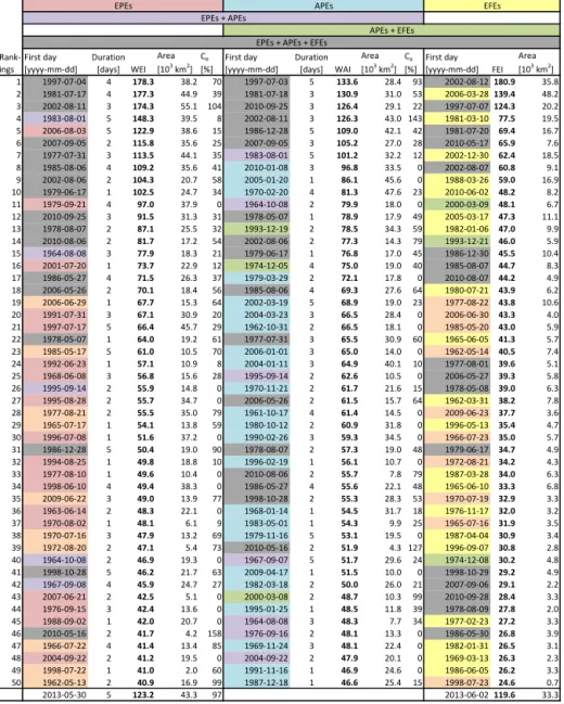
Although the WEI, the WAI, and the FEI itself are indepen-dent of thresholds, it was necessary to limit their values to constrain the sets of events that would be classified as EPEs, APEs, and EFEs. This step was performed because there are no natural limits dividing extreme from non-extreme events. In fact, the extremity of events gradually decreases with even smaller differences among the events as less-extreme events are considered. We selected the 50 events of each type so that one extreme event occurs per year on average. Sets of EPEs, APEs, and EFEs during the period of 1961–2010 in the Czech Republic are listed in Fig. 6.
pro- Rank-ings
First day [yyyy-mm-dd]
Duration [days] WEI
Area [103 km2]
Ce
[%] First day [yyyy-mm-dd]
Duration [days] WAI
Area [103 km2]
Ca
[%] First day [yyyy-mm-dd] FEI
Area [103 km2] 1 1997-07-04 4 178.3 38.2 70 1997-07-03 5 133.6 28.4 93 2002-08-12180.9 35.8 2 1981-07-17 4 177.3 44.9 39 1981-07-18 3 130.9 31.0 53 2006-03-28139.4 48.2 3 2002-08-11 3 174.3 55.1 104 2010-09-25 3 126.4 29.1 22 1997-07-07124.3 20.2 4 1983-08-01 5 148.3 39.5 8 2002-08-11 3 126.3 43.0 143 1981-03-10 77.5 19.5 5 2006-08-03 5 122.9 38.6 15 1986-12-28 5 109.0 42.1 42 1981-07-20 69.4 16.7 6 2007-09-05 2 115.8 35.6 25 2007-09-05 3 105.2 27.0 28 2010-05-17 65.9 7.6 7 1977-07-31 3 113.5 44.1 35 1983-08-01 5 101.2 32.2 12 2002-12-30 62.4 18.5 8 1985-08-06 4 109.2 35.6 41 2010-01-08 3 96.8 33.5 0 2002-08-07 60.8 9.1 9 2002-08-06 2 104.3 20.7 58 2005-01-20 1 86.1 45.6 0 1988-03-26 59.0 16.9 10 1979-06-17 1 102.5 24.7 34 1970-02-20 4 81.3 47.6 23 2010-06-02 48.2 8.2 11 1979-09-21 4 97.0 37.9 0 1964-10-08 2 79.9 18.0 0 2000-03-09 48.1 6.7 12 2010-09-25 3 91.5 31.3 31 1978-05-07 1 78.9 17.9 49 2005-03-17 47.3 11.1 13 1978-08-07 2 87.1 25.5 32 1993-12-19 2 78.5 34.3 59 1982-01-06 47.0 9.9 14 2010-08-06 2 81.7 17.2 54 2002-08-06 2 77.3 14.3 79 1993-12-21 46.0 5.9 15 1964-08-08 3 77.9 18.3 21 1979-06-17 1 76.8 17.0 45 1986-12-30 45.5 10.4 16 2001-07-20 1 73.7 22.9 12 1974-12-05 4 75.0 19.0 40 1985-08-07 44.7 8.3 17 1986-05-27 4 71.5 26.3 37 1979-03-29 2 72.1 17.8 0 2010-08-07 44.2 4.9 18 2006-05-26 2 70.1 18.4 56 1985-08-06 4 69.3 27.6 64 1980-07-21 43.9 6.2 19 2006-06-29 1 67.7 15.3 64 2002-03-19 5 68.9 19.0 23 1977-08-22 43.8 10.6 20 1991-07-31 3 67.1 30.9 20 2004-03-23 3 66.5 28.4 0 2006-06-30 43.3 4.0 21 1997-07-17 5 66.4 45.7 29 1962-10-31 2 66.5 18.1 0 1985-05-20 43.0 5.9 22 1978-05-07 1 64.0 19.2 61 1977-07-31 3 65.5 30.9 60 1965-06-05 41.3 5.7 23 1985-05-17 5 61.0 10.5 70 2006-01-01 3 65.0 14.0 0 1962-05-14 40.5 7.4 24 1992-06-23 1 57.1 10.9 8 2004-01-11 3 64.9 40.1 10 1977-08-01 39.6 5.1 25 1968-06-08 3 56.8 15.6 28 1995-09-14 2 62.6 10.5 0 2006-05-27 39.3 5.8 26 1995-09-14 2 55.9 14.8 0 1970-11-21 2 61.7 21.6 15 1978-05-08 39.0 6.3 27 1995-08-28 2 55.7 34.7 0 2006-05-26 2 61.5 15.7 64 1962-03-31 38.2 7.8 28 1977-08-21 2 55.5 35.0 79 1961-10-17 4 61.4 14.5 0 2009-06-23 37.7 3.6 29 1965-07-17 1 54.1 13.8 59 1980-10-12 2 60.9 31.8 0 1996-05-13 35.4 4.7 30 1996-07-08 1 51.6 37.2 0 1990-02-26 3 59.3 34.5 0 1966-07-23 35.0 5.7 31 1986-12-28 5 50.4 19.0 90 1978-08-07 2 57.3 19.0 48 1979-06-17 34.7 4.9 32 1994-08-25 1 49.8 18.8 10 1996-02-19 1 56.1 10.7 0 1972-08-21 34.2 4.3 33 1977-08-10 1 49.6 10.4 0 2010-08-06 2 55.7 7.8 79 1987-03-28 34.0 6.3 34 1998-06-10 4 49.4 38.3 0 1986-05-27 4 55.6 22.1 48 1965-06-10 33.3 6.8 35 2009-06-22 3 49.0 13.9 77 1998-10-28 2 55.3 28.3 53 1970-07-19 32.9 3.3 36 1963-06-14 2 48.3 22.1 0 1968-01-14 1 54.5 31.7 18 1976-11-17 32.0 3.2 37 1970-08-02 1 48.1 6.1 9 1983-05-01 1 54.3 9.9 25 1965-07-16 31.9 3.5 38 1970-07-16 3 47.9 13.2 69 1979-11-16 5 53.1 19.5 0 1987-04-04 30.9 3.4 39 1972-08-20 2 47.1 5.4 73 2010-05-16 2 51.9 4.3 127 1996-09-07 30.8 2.8 40 1964-10-08 2 46.9 19.3 0 1967-09-07 5 51.7 29.6 24 1974-12-08 30.2 4.8 41 1998-10-28 5 46.2 21.7 63 2009-04-17 1 51.5 10.0 0 1998-10-29 29.2 4.9 42 1967-09-08 4 45.9 24.7 27 1982-03-18 2 50.0 26.0 21 2007-09-06 29.1 2.2 43 2007-06-21 2 42.5 5.1 0 2000-03-08 2 48.7 10.3 99 2010-09-28 28.4 3.3 44 1976-09-15 3 42.4 13.6 0 1995-01-25 1 48.5 11.8 39 1978-08-09 27.8 2.0 45 1988-09-02 1 42.0 20.7 0 1964-08-08 3 48.3 7.7 34 1977-02-23 27.2 3.3 46 2010-05-16 2 41.7 4.2 158 1976-09-16 2 48.1 13.3 0 1986-05-30 26.8 3.9 47 1966-07-22 4 41.4 13.4 85 1969-11-24 3 48.1 22.4 0 1982-01-31 26.5 3.1 48 2004-09-22 2 41.2 19.5 0 2004-09-22 2 47.9 20.1 0 1969-03-13 26.3 2.3 49 1998-07-22 1 41.0 2.0 60 1991-11-16 1 46.9 24.6 0 1986-06-05 26.2 3.3 50 1962-05-13 2 40.9 16.9 99 1987-12-18 1 46.6 25.4 15 1998-07-23 24.6 0.7
2013-05-30 5 123.2 43.3 97 2013-06-02119.6 33.3
EPEs + APEs + EFEs
EPEs APEs EFEs
EPEs + APEs
APEs + EFEs
Figure 6. EPEs, APEs, and EFEs in the Czech Republic, 1961–2010. Colors denote the assignment of events to one or more types of
extremes; the ratios of the FEI to the WEI and to the WAI are designated theCeandCa, respectively. For comparison, an extra event from
May–June 2013 is represented by values of the WEI and the FEI.
duced by EPEs increases to 75 %. This fact suggests that the magnitude of causal precipitation is the main factor condi-tioning most of floods in the Czech Republic. Nevertheless, we also identified cases in which the hydrological response to an EPE was too small or too big. These events confirm that flooding is also significantly influenced by other factors, which are further discussed in Sect. 4.2.
3.2 Inter-annual variability of extremes
The temporal distribution of extreme events during the pe-riod of 1961–2010 is shown in Fig. 7. Regardless of the type of extremes (EPEs, APEs, and EFEs), there are certain com-mon features of their variations in time. One such feature is
the below-normal frequency and magnitude of all types of extremes during the first 16 years of this time period. The situation dramatically changed in 1977, when three EPEs oc-curred in the span of less than 1 month; two of them produced EFEs (Fig. 6). Similar conditions occurred during the follow-ing 2 years. Moreover, the second and the fourth highest val-ues of the WEI were recorded in July 1981 and August 1983, respectively. The wet years of 1985–1986 ended a decade of all types of extremes with above-normal frequency and mag-nitude.
0 0.25 0.5 0.75 1
0 25 50 75 100 125 150 175 200
1961 1971 1981 1991 2001 2011
WE
I, W
AI,
FEI
F(c) F(w)
1d 2d
3d 4d
5d 1d
2d 3d
4d 5d
EFEs EFEs (w) APEs EPEs
Figure 7. Temporal variability of extreme events, 1961–2010, in
the Czech Republic. The red, blue, dark green, and light green sym-bols denote EPEs, APEs, EFEs during colder half of the year (ND-JFMA), and EFEs during warmer half of the year (MJJASO), re-spectively. The symbol shapes denote the duration (no. of days) of EPEs and APEs. The curves express relative cumulative values (right axis) of the WEI, the WAI, and the FEI (dark green denotes all seasons, light green denotes warmer half-years only).
not occur again until 1996. The rest of the 1990s would also be considered to be below normal if July 1997 were not in-cluded. The first of two EPEs in this month exhibited maxi-mum values of both the WEI and WAI. Similar values were also observed 5 years later, in August 2002. Compared to similarly strong precipitation events in the early 1980s, these two events produced much greater flooding. The last 5 years of the study period were characterized by an abnormally high number of extremes, which were concentrated primarily in 2006 and 2010. If the 2013 flood were considered, four max-imum EFEs occurred recently approximately every 5 years.
3.3 Seasonal distribution of extremes
The seasonal distribution of EPEs was significantly unequal during the period of 1961–2010 (Fig. 8). Based on the se-lected threshold, these events occurred from May to Decem-ber. Nevertheless, only three such events occurred since Oc-tober, all rather weak. The months of greatest activity were clearly July and August, when the five highest values of WEI were noted. The level of activity during the first half of Au-gust was particularly pronounced: this time period was the seasonal peak in EPEs during the period of 1961–2010.
Naturally, APEs were distributed more equally from sea-son to seasea-son during the 1961–2010 period than were the EPEs (Fig. 8). We noted at least one event in every calen-dar month. From October to March, the distribution of APEs was very uniform in terms of both the number of events and the magnitude. The values of the WAI were less than 100 with only one exception, which occurred during the 5 days from 28 December 1986 to 1 January 1987. This event was
Figure 8.Seasonal distribution of extreme events in the Czech
Re-public, 1961–2010. EPEs were evaluated using the WEI (red), APEs using the WAI (blue), and EFEs using the FEI (green). Values of the indices are depicted by the distance of symbols from the center of the diagram. The shape of symbols depicts how many days the pre-cipitation event lasted.
so exceptional that it also qualified as an EPE (see above). In contrast, only one APE was noted in April. This event and two others in the first half of May lasted only 1 day each.
4 Discussion of results
4.1 Comparison with standard indices
In this section, the presented evaluation of precipitation and flood events is compared with standard methods mentioned in Sect. 1.
Regarding precipitation extremes, they are usually de-tected by maximum daily totals P1 at any individual rain gauge (Ustrnul et al., 2015) or by areal precipitation means
Ad during d days, for example, for d=2 days (Konrad,
2001). The first approach is commonly used in the Czech Re-public: Štekl et al. (2001) analyzed days during the period of 1876–2000 when a daily total reached at least 150 mm any-where in the Czech Republic. The Czech maximum occurred on 29 July 1897 when a P1 of 345.1 mm was measured at
the Nová Louka gauge in the Jizerské Hory Mts. Indeed, this event was the maximumP1ever recorded in central Europe
(Munzar et al., 2011).
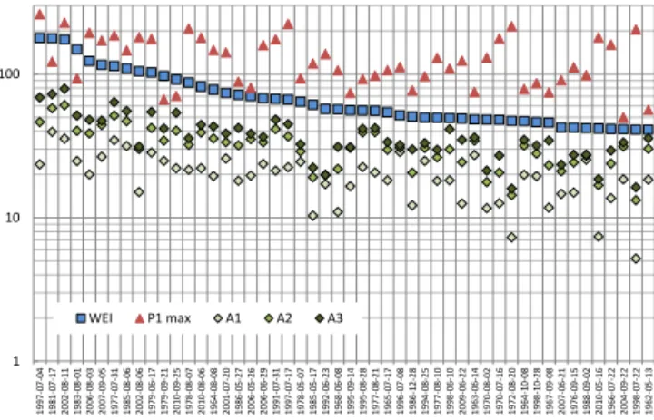
Figure 9 compares 50 maximum WEI values with maxi-mumP1and areal 1-, 2-, and 3-day means during the EPEs.
It demonstrates that areal precipitation means generally de-crease with decreasing WEI values, but it is not fully true for point daily totals. As a result, the ranking of precipitation events significantly depends on the evaluation criterion. For example, daily point maxima were above 200 mm on 20 Au-gust 1972 and 22 July 1998 but the 1-day areal means were only 5.2 and 7.3 mm, respectively. The affected area was very small in both cases (see Fig. 6). In 1972, strong precipitation affected a large area but mainly outside the Czech state bor-der (Müller et al., 2009), whereas the 1998 case was due to a strong convective storm within a limited area ( ˇRezáˇcová and Sokol, 2003). Thus, the WEI seems to be a good compromise between the two standard approaches.
In contrast, there were many significant EPEs with high areal totals but without any point daily total exceeding 150 mm. For example, the second largest EPE in July 1981 was characterized by P1 of only 122.0 mm but extra high areal totals (absolute maximum of A1) produced the third largest EFE during MJJASO (Fig. 6). A still lower daily max-imum (only 97.6 mm) was recorded during the historical case on 2 September 1890 when the 3-day areal precipitation to-tal (1–3 September) was nearly as high as in August 2002 and subsequent flooding was only slightly less catastrophic ( ˇRezáˇcová et al., 2005a). The WEI reached very high value in July 1981 because the index reflects the size of the affected area and the fact that heavy rains occurred not only in moun-tains but also in lowlands where they are rare.
Moreover, some precipitation events lasted virtually only 1 day (e.g., 23 June 1992) but others lasted 3 or even more days (e.g., 4–7 July 1997). The first case is not properly evaluated by the areal 3-day mean total and the latter by the areal 1-day mean while the WEI accommodates to the real duration of the events. All abovementioned examples demonstrate the advantage of the WEI, which combines the intensity of
pre-1 10 100 1 9 9 7 -0 7 -0 4 1 9 8 1 -0 7 -1 7 2 0 0 2 -0 8 -1 1 1 9 8 3 -0 8 -0 1 2 0 0 6 -0 8 -0 3 2 0 0 7 -0 9 -0 5 1 9 7 7 -0 7 -3 1 1 9 8 5 -0 8 -0 6 2 00 2-0 8-0 6 1 9 7 9 -0 6 -1 7 1 9 7 9 -0 9 -2 1 2 0 1 0 -0 9 -2 5 1 9 7 8 -0 8 -0 7 2 0 1 0 -0 8 -0 6 1 9 6 4 -0 8 -0 8 2 0 0 1 -0 7 -2 0 1 9 8 6 -0 5 -2 7 2 0 0 6 -0 5 -2 6 2 0 0 6 -0 6 -2 9 1 9 9 1 -0 7 -3 1 1 9 9 7 -0 7 -1 7 1 9 7 8 -0 5 -0 7 1 9 8 5 -0 5 -1 7 1 9 9 2 -0 6 -2 3 1 9 6 8 -0 6 -0 8 1 9 9 5 -0 9 -1 4 1 9 9 5 -0 8 -2 8 1 9 7 7 -0 8 -2 1 1 9 6 5 -0 7 -1 7 1 9 9 6 -0 7 -0 8 1 9 8 6 -1 2 -2 8 1 99 4-0 8-2 5 1 9 7 7 -0 8 -1 0 1 9 9 8 -0 6 -1 0 2 0 0 9 -0 6 -2 2 1 9 6 3 -0 6 -1 4 1 9 7 0 -0 8 -0 2 1 9 7 0 -0 7 -1 6 1 9 7 2 -0 8 -2 0 1 9 6 4 -1 0 -0 8 1 9 9 8 -1 0 -2 8 1 9 6 7 -0 9 -0 8 2 0 0 7 -0 6 -2 1 1 9 7 6 -0 9 -1 5 1 9 8 8 -0 9 -0 2 2 0 1 0 -0 5 -1 6 1 9 6 6 -0 7 -2 2 2 0 0 4 -0 9 -2 2 1 9 9 8 -0 7 -2 2 1 9 6 2 -0 5 -1 3
WEI P1 max A1 A2 A3
Figure 9.EPEs characterized by the WEI, maximum daily
precip-itation total [mm] at a site (P1), and areal mean precipitation total
[mm] in the Czech Republic recorded during 1 day (A1), 2 days
(A2), and 3 days (A3).
cipitation with its spatial extent and reflects also duration of precipitation events.
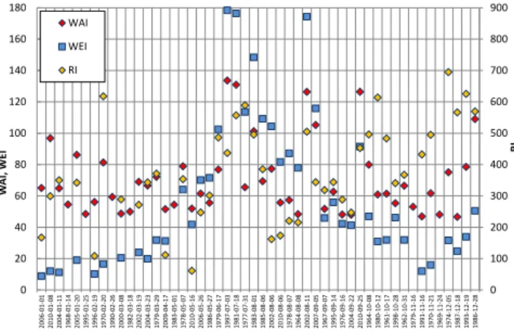
Precipitation extremes are usually evaluated regardless the season when they occurred. Recently, Ramos et al. (2014) suggested an index ranking daily precipitation extremes, which employs 1-day precipitation totals normalized by their climatology on the given calendar day. The index can be hardly compared with the WAI because Ramos et al. (2014) do not reflect duration of precipitation events. Nevertheless, we decided to accumulate daily values of their index on indi-vidual days of the APEs and compare the sums (hereinafter called RI) with the WAI values (Fig. 10).
Naturally, the WAI is more closely related to the WEI than the RI. Values of the WAI are higher than the WEI from September to the middle of May and lower in the rest of the year. Values of the RI seem to be a bit more equally dis-tributed through the calendar year but they correspond less to the precipitation extremity. It can be demonstrated by the comparison of two July events: the maximum EPE from the beginning of July 1997 is represented by only the 16th high-est RI value but significantly less extreme event from 1977 reached the 6th highest value of the RI though the turn of July and August is the top season of heavy rains in the Czech Republic. A possible reason can be the fact that daily precip-itation totals are not normally distributed but the RI standard-izes them only by the mean and the variance.
(here-0 100 200 300 400 500 600 700 800 900 0 20 40 60 80 100 120 140 160 180 20 06- 01-01 20 10- 01-08 20 04- 01-11 19 68- 01-14 20 05- 01-20 19 95- 01-25 19 96- 02-19 19 70- 02-20 19 90 -02 -26 20 00- 03-08 19 82- 03-18 20 02- 03-19 20 04- 03-23 19 79- 03-29 20 09- 04-17 19 83 -05 -01 19 78- 05-07 20 10- 05-16 20 06- 05-26 19 86- 05-27 19 79- 06-17 19 97- 07-03 19 81- 07-18 19 77- 07-31 19 83- 08-01 19 85- 08-06 20 02- 08-06 20 10- 08-06 19 78- 08-07 19 64- 08-08 20 02- 08-11 20 07- 09-05 19 67- 09-07 19 95- 09-14 19 76- 09-16 20 04- 09-22 20 10- 09-25 19 64- 10-08 19 80 -10 -12 19 61- 10-17 19 98- 10-28 19 62- 10-31 19 79- 11-16 19 91- 11-16 19 70- 11-21 19 69 -11 -24 19 74- 12-05 19 87- 12-18 19 93- 12-19 19 86- 12-28 RI W A I, WEI WAI WEI RI
Figure 10. APEs characterized by the WAI, the WEI, and values
of the index RI according to Ramos et al. (2014). The 50 APEs are ordered with respect to the calendar day in the increasing order.
inafter FEI_8). Only 31 of EFEs reached the FEI_8 values above zero (Fig. 11). Even such a rough comparison of the indices shows that the FEI is a compromise between the FI representing the most affected catchment and the UI, which emphasizes the size of the affected area even more than the FEI. The difference between the FI and the UI was mainly evident in July 1997 when the floods were extreme in the eastern part of the Czech Republic but no flood occurred in the western part.
4.2 Relationship between precipitation extremes and
floods
Though many precipitation extremes correspond with EFEs, there are still discrepancies between the WEI and the FEI and even greater discrepancies between the WAI and the FEI val-ues. For example, the fourth largest EPE did not produce an EFE in August 1983; in fact, this EPE resulted in very lim-ited flooding (Ce=8 %; see Fig. 6). Several factors affected
the hydrological response of this event. These include un-usually low antecedent saturation (mean API30only 9.3 mm) and a moderately even distribution of rainfall over 5 days, whose maximum occurred on the second day of the event. Regulation processes by the dams could also play a role; nevertheless, Brázdil et al. (2005) confirm that no even un-affected peak flow with the return period of 2 or more years occurred at Vltava River in Prague even though the catch-ment belonged to the most affected by heavy rains.
All these factors will be studied in the future together with spatial patterns of precipitation to elucidate the discrepancies between individual precipitation and flood events. One of the factors to be considered should be the season when an EPE occurred, as discussed in Sect. 3.3. The important role of this factor is confirmed by Fig. 12. It is clear that the hydrological effect of an EPE is typically strong in May, more ambiguous in summer, and considerably weaker in September. The very last event from the turn of May and June 2013 also supports
0 1 2 3 4 10 100 1000 2 0 0 2 -0 8 -1 2 2 0 1 3 -0 6 -0 2 2 0 0 6 -0 3 -2 8 1 9 9 7 -0 7 -0 7 1 9 8 1 -0 7 -2 0 1 9 8 8 -0 3 -2 6 2 0 1 0 -0 5 -1 7 2 0 1 0 -0 6 -0 2 1 9 8 1 -0 3 -1 0 1 9 8 2 -0 1 -0 6 1 9 7 7 -0 2 -2 3 2 0 0 2 -0 8 -0 7 1 9 7 0 -0 7 -1 9 1 9 8 5 -0 8 -0 7 2 0 0 2 -1 2 -3 0 1 9 8 6 -1 2 -3 0 1 9 7 4 -1 2 -0 8 1 9 8 5 -0 5 -2 0 1 9 8 7 -0 3 -2 8 1 9 9 3 -1 2 -2 1 1 9 6 2 -0 3 -3 1 1 9 6 6 -0 7 -2 3 1 9 6 5 -0 6 -1 0 1 9 8 6 -0 6 -0 5 2 0 0 6 -0 5 -2 7 1 9 7 8 -0 5 -0 8 1 9 8 6 -0 5 -3 0 1 9 7 7 -0 8 -0 1 1 9 7 2 -0 8 -2 1 1 9 8 0 -0 7 -2 1 2 0 0 9 -0 6 -2 3 FI , UI FE I_8
FEI_8 FI UI
Figure 11.EFEs characterized by the FEI, the index by Uhlemann
et al. (2010) (UI), and by the maximum Francou index (FI) calcu-lated within eight selected large Czech catchments.
Figure 12.Relationship between rankings of 50 maximum EPEs
(left)/APEs (right) and rankings of subsequent floods in various months (distinguished by colors). Precipitation events, whose hy-drological response was too small (no peak flow with return period at least 5 years), are depicted at the top of the diagram.
this conclusion (Ce=97 %; see Fig. 6). If an EPE occurs
in the last month of the year, it can also produce rather big flooding, although such events are very rare.
The hydrological effect of APEs (Fig. 12) is substantially reduced in the winter, early spring (most likely due to pre-cipitation in the form of snow), and autumn. In contrast, if precipitation events are sufficiently high to qualify as APEs in the late spring and summer, they are usually flood pro-ducing; surprisingly, this was also the case with all APEs in December. A subsequent detailed study of intra-annual vari-ations in precipitation patterns is necessary to explain these findings.
this has occurred six times since 1997 (Fig. 7). Several fac-tors most likely explain the difference: (i) if two or more EPEs appeared during one year in the first period, they were separated by a much longer interval than in the latter period (the shortest interval between two EPEs was 8 days in 1977 but only 3 days in 2002); (ii) in cases of EPEs following one after another, the magnitude decreased in the first period (WEI decreasing from 113.5 to 49.6 in July/August 1977) but increased in the second period (WEI increasing from 104.3 to 174.3 in August 2002); (iii) just before the main EPEs, the mean antecedent saturation was much lower on 17 July 1981 (24.6 mm) and on 1 August 1983 (9.3 mm) than on 4 July 1997 (34.5 mm) and on 11 August 2002 (50.1 mm because of the above-mentioned preceding EPE); and (iv) the EPEs in 1981 and 1983 lasted 1 day longer than those in 1997 and 2002. It demonstrates that changes in a flood regime can also occur without significant changes in only the magnitude of precipitation events.
5 Conclusions
The paper presents three indices for evaluation of hydrom-eteorological extremes. In contrast to common indices, the presented indices reflect not only maxima of precipitation amounts and peak discharges at individual gauges but also the rarity of values, the size of the affected area, and the dura-tion of precipitadura-tion. Besides that, the aspect of precipitadura-tion seasonality was considered, which enables the detection of precipitation extremes throughout the year. A unified design of the presented indices enables one to easily compare inter-annual and seasonal distributions of precipitation extremes and large floods.
The application of the indices to the Czech territory demonstrates that this approach enables one to compare the extremity of precipitation and consequent floods rather than when precipitation events are evaluated only by the maxi-mum precipitation total at one station. Extreme floods cor-respond to precipitation extremes; nevertheless, not only the magnitude of precipitation extremes influences the hydrolog-ical response but also the season, the antecedent saturation and other factors. The study confirms that variations in the frequency and/or magnitude of floods can be due to not only variations in the magnitude of precipitation events but also variations in these factors.
Additional detailed studies are necessary for elucidating the way in which seasonality influences the hydrological ef-fect of precipitation extremes. This efef-fect could be due to seasonal differences in evapotranspiration or to possible sea-sonal variations in the attributes of the precipitation itself. The events can differ, e.g., in the spatial distribution of pre-cipitation within the affected area or in the temporal con-centration of precipitation during the event (intensity can in-crease, remain the same or decrease). In addition, various cir-culation conditions could explain the differences among the
extremes (Kašpar and Müller, 2010). In a next step, we plan to explore the dependences on the circulation extremity in-dex (Kašpar and Müller, 2014), which completes the set of tools for studying the pathway of causation from circulation to precipitation and runoff.
Acknowledgements. The research presented in this study is
supported by the Czech Science Foundation under the GACR P209/11/1990 project. Precipitation and runoff data were provided by the Czech Hydrometeorological Institute. We would also like to thank J. Kyselý and L. Gaál from the Institute of Atmospheric Physics in Prague for implementing the ROI method.
Edited by: U. Ehret
References
Alexander, L. V., Zhang, X., Peterson, T. C., Caesar, J., Gleason, B., Klein Tank, A. M. G., Haylock, M., Collins, D., Trewin, B., Rahimzadeh, F., Tagipour, A., Rupa Kumar, K., Revadekar, J., Griffiths, G., Vincent, L., Stephenson, D. B., Burn, J., Aguilar, E., Brunet, M., Taylor, M., New, M., Zhai, P., Rusticucci, M., and Vazquez-Aguirre, J. L.: Global observed changes in daily climate extremes of temperature and precipitation, J. Geophys. Res., 111, D05109, doi:10.1029/2005JD006290, 2006.
Barredo, J. I.: Major flood disasters in Europe: 1950–2005, Nat. Hazards, 42, 125–148, 2007.
Begueria, S., Vicente-Serrano, S. M., Lopez-Moreno, J. I., and Garcia-Ruiz, J. M.: Annual and seasonal mapping of peak in-tensity, magnitude and duration of extreme precipitation events across a climatic gradient, northeast Spain, Int. J. Climatol., 29, 1759–1779, 2009.
Black, A. R. and Werritty, A.: Seasonality of flooding: a case study of North Britain, J. Hydrol., 195, 1–25, 1997.
Blinchikoff, H. J. and Zverev, A. I.: Filtering in the time and fre-quency domain, Scitech Publishing, Raleigh, USA, 2001. Brázdil, R., Dobrovolný, P., Elleder, L., Kakos, V., Kotyza, O.,
Kvˇetoˇn, V., Macková, J., Müller, M., Štekl, J., Tolasz, R., and Valášek, H.: Historical and recent floods in the Czech Republic, in: History of weather and climate in the Czech lands, vol. 7, Masaryk University, Brno, Czech Republic, 370 pp., 2005. Burn, D. H.: Evaluation of regional flood frequency analysis with
a region of influence approach, Water Resour. Res., 26, 2257– 2265, 1990.
ˇCekal, R. and Hladný, J.: Analysis of flood occurrence seasonality on the Czech Republic territory with directional characteristics method, AUC Geographica, 43, 3–14, 2008.
Herschy, R. W. (Ed.): World catalogue of maximum observed floods, IAHS Press, Wallingford, IAHS-AISH Publ. 284,
285 pp.+supplement, 2003.
Hosking, J. R. M. and Wallis, J. R.: Regional Frequency Analy-sis: An Approach Based on L-Moments, Cambridge University Press, New York, 1997.
Kašpar, M. and Müller, M.: Variants of synoptic patterns inducing heavy rains in the Czech Republic, Phys. Chem. Earth, 35, 477– 483, 2010.
Kašpar, M. and Müller, M.: Combinations of large-scale circulation anomalies conducive to precipitation extremes in the Czech Re-public, Atmos. Res., 138, 205–212, 2014.
Köhler, M. A. and Linsley, R. K.: Predicting the runoff from storm rainfall, US Weather Bureau Research Paper no. 34., Washing-ton, 9 pp., 1951.
Konrad, C. E.: The most extreme precipitation events over the East-ern United States from 1950 to 1996: Considerations of scale, J. Hydrometeorol., 2, 309–325, 2001.
Kyselý, J. and Picek, J.: Regional growth curves and improved de-sign value estimates of extreme precipitation events in the Czech Republic, Clim. Res., 33, 243–255, 2007.
Kyselý, J., Gaál, L., and Picek, J.: Comparison of regional and at-site approaches to modelling probabilities of heavy precipitation, Int. J. Climatol., 31, 1457–1472, 2011.
Langhammer, J.: Modelling the impact of anthropogenic modifi-cations to river channels on the course of extreme floods. Case study: August 2002 flood, Blanice River basin, Czechia, Ge-ografie, 113, 237–252, 2008.
Müller, M. and Kašpar, M.: Event-adjusted evaluation of weather and climate extremes, Nat. Hazards Earth Syst. Sci., 14, 473– 483, doi:10.5194/nhess-14-473-2014, 2014.
Müller, M., Kašpar, M., and Matschullat, J.: Heavy rains and extreme rainfall-runoff events in Central Europe from 1951 to 2002, Nat. Hazards Earth Syst. Sci., 9, 441–450, doi:10.5194/nhess-9-441-2009, 2009.
Munzar, J., Ondráˇcek, S., and Auer, I.: Central European one-day precipitation records, Moravian Geographical Reports, 19, 32– 40, 2011.
Ramos, A. M., Trigo, R. M., and Liberato, M. L. R.: A ranking of high-resolution daily precipitation extreme events for the Iberian Peninsula, Atmos. Sci. Let., 15, 328–334, 2014.
Ren, F. M., Cui, D. L., Gong, Z. Q., Wang, Y. J., Zou, X. K., Li, Y. P., Wang, S. G., and Wang, X. L.: An objective identification tech-nique for regional extreme events, J. Climate, 25, 7015–7027, 2012.
ˇRezáˇcová, D. and Sokol, Z.: A diagnostic study of a summer con-vective precipitation event in the Czech Republic using a nonhy-drostatic NWP model, Atmos. Res., 67–68, 559–572, 2003 ˇRezáˇcová, D., Kašpar, M., Müller, M., Sokol, Z., Kakos, V.,
Hanslian, H., and Pešice, P.: A comparison of flood precipita-tion in August 2002 with historical extreme precipitaprecipita-tion events from the Czech territory, Atmos. Res., 77, 354–366, 2005a. ˇRezáˇcová, D., Pešice, P., and Sokol, Z.: An estimation of the
proba-ble maximum precipitation for river basins in the Czech Repub-lic, Atmos. Res., 77, 407–421, 2005b.
Rodier, J. A. and Roche, M. (Eds.): World catalogue of maximum observed floods, IAHS Press, Wallingford, IAHS Publ. 143, 1984.
Šercl, P., Tyl, R., and Pecha, M.: The course and the extremity of the June 2013 floods, Meteorologické zprávy, 66, 197–202, 2013. Štekl, J., Brázdil, R., Kakos, V., Jež, J., Tolasz, R., and Sokol, Z.:
Extreme daily precipitation totals during 1879–2000 in the Czech territory a their synoptic causes, Národní klimatický program
ˇCeské republiky 31, Prague, Czech Republic, 140 pp., 2001. Stephenson, D. B.: Definition, diagnosis, and origin of extreme
weather and climate events, in: Climate Extremes and Society, edited by: Diaz, H. F. and Murnane, R. J., Cambridge University Press, New York, 11–23, doi:10.1017/CBO9780511535840.004, 2008.
Tolasz, R., Míková, T., Valeriánová, A., and Voženílek, V. (Eds.): Climate atlas of Czechia, Czech Hydrometeorological Institute, Prague, Czech Republic, 256 pp., 2007.
Uhlemann, S., Thieken, A. H., and Merz, B.: A consistent set of trans-basin floods in Germany between 1952–2002, Hy-drol. Earth Syst. Sci., 14, 1277–1295, doi:10.5194/hess-14-1277-2010, 2010.
Ustrnul, Z., Wypych, A., Henek, E., Maciejewski, M., and Boch-enek, B.: Climatologically based warning system against meteo-rological hazards and weather extremes: the example for Poland, Nat. Hazards, 77, 1711–1729, 2015.