www.nonlin-processes-geophys.net/14/641/2007/ © Author(s) 2007. This work is licensed
under a Creative Commons License.
Nonlinear Processes
in Geophysics
Venus atmosphere profile from a maximum entropy principle
L. N. Epele1, H. Fanchiotti1, C. A. Garc´ıa Canal1, A. F. Pacheco2, and J. Sa ˜nudo3
1Laboratorio de F´ısica Te´orica, Departamento de F´ısica, IFLP, Facultad de Ciencias Exactas, Universidad Nacional de La Plata C.C. 67, 1900 La Plata, Argentina
2Facultad de Ciencias and BIFI, Universidad de Zaragoza, 50009 Zaragoza, Spain 3Departamento de F´ısica, Universidad de Extremadura, Badajoz, Spain
Received: 25 April 2007 – Accepted: 6 July 2007 – Published: 18 October 2007
Abstract. The variational method with constraints recently developed by Verkley and Gerkema to describe maximum-entropy atmospheric profiles is generalized to ideal gases but with temperature-dependent specific heats. In so doing, an extended and non standard potential temperature is intro-duced that is well suited for tackling the problem under con-sideration. This new formalism is successfully applied to the atmosphere of Venus. Three well defined regions emerge in this atmosphere up to a height of 100 km from the surface: the lowest one up to about 35 km is adiabatic, a transition layer located at the height of the cloud deck and finally a third region which is practically isothermal.
1 Introduction
Since the late 1950s, there have been hundreds of space ex-ploration missions that have provided data on the composi-tion, structure and circulation of planetary atmospheres. In particular, the vertical pressure-temperature profile of the at-mosphere of Venus was accurately observed in the Pioneer-Venus II mission in 1978 (Seiff et al., 1980). In Landis et al. (2002), an averaged data of temperature, pressure and density of the Venus atmosphere as a function of altitude above the surface is given. In this paper we will use this information.
On Venus, the incoming solar energy, of the order of 2600 W/m2, is almost twice as great as on Earth. Venus pos-sess an atmosphere, which is about a hundred times as mas-sive as that of the Earth and its surface temperature reaches 730 K. Carbon dioxide is the major component (96.5 per cent), and 3.5 per cent of N2 is the next most abundant species.
In a recent paper by Verkley and Gerkema (2004), hence-forth denoted by VG, have proposed a first-principles varia-Correspondence to: L. N. Epele
tional method to generate ap−T profile for an atmospheric column. This profile is the result of maximizing the entropy of the column,S, maintaining fixed its mass,M, enthalpy,H, and the integral of the potential temperature,L. This method is flexible enough to describe from an isothermal profile to an adiabatic one depending on the value of a unique param-eter. VG applied these ideas to the Earth’s troposphere and accurately reproduced the U.S. Standard Atmosphere.
In their analysis, VG considered that the atmospheric gas is ideal, i.e. a gas that verifies the corresponding equation of state, and besides, the specific heats,CV ,p, are constant. When this second assumption is also fulfilled it is said that the gas is perfect. These two hypotheses are quite reason-able when dealing with the atmosphere of the Earth. For rep-resentative temperatures and pressures of the low Venus at-mosphere, however, the temperature dependence of theCV ,p
has to inescapably be taken into account. As our goal in this paper is the application of the VG ideas to the Venus atmosphere, we have had to extend their original variational method to take into account this dependence of the specific heats on temperature. Consequently we will first extend the VG method to ideal imperfect gases. As is well known, the temperature dependence of theCV ,pcomes from the
excita-tion of some internal vibraexcita-tional levels of the molecule when the temperature is high enough.
Throughout the paper we will consider that CO2 is the main chemical component of the Venus atmosphere. The chemical impurities coming from the N2 produce negligi-ble corrections in our analysis. Besides, we will not con-sider any correction coming from the interaction between the molecules, that is, we will stick to the scenario of an ideal gas but with the afore-mentioned temperature dependence of the
CV ,p. Corrections of real gas in the Venus atmosphere have
equation of state of ideal gases is good to describe the gas of Venus can be done using the data of Landis et al. (2002). There one can check, at each height, that using pressure and temperature as input, the value of density obtained from the equation of the ideal gases is, in all cases, equal to the exper-imental value with a discrepancy lower than 2 per cent.
The index of the paper is as follows. In Sect. 2, we will recall the meaning of the potential temperature,θ, for ideal perfect gases and its relation to the entropy. In Sect. 3, we will review the VG method and comment on the main re-sults when it is applied to the Earth’s troposphere. In Sect. 4, we will put in evidence the necessity of considering an ex-plicit dependence of theCV ,pwith temperature for the CO2 molecule, to properly describe the Venus atmosphere. In Sect. 5, we will calculate the equation of the potential tem-perature, i.e. the form of an adiabatic, when dealing with ideal-imperfect gases. In Sect. 6, we will extend the VG method to ideal-imperfect gases. In Sect. 7, this new method will be applied to the Venus atmosphere and the results will be commented on. Finally, in Sect. 8 we present our conclu-sions.
2 The potential temperature and the entropy for ideal perfect gases
The first principle of Thermodynamics says that
δU=δQ−p δV . (1)
Throughout this paper,δindicates all the variations of ther-modynamical quantities, whereasd will be used to refer to variations of quantities at different altitudes.
For ideal gases, the equation of state, for 1 mol, is
p V =R∗T (2)
(whereR∗=8.3143 J mol−1K−1is the universal gas constant) and the specific internal energy (internal energy per unit mass, noted with lower case letter) reads
u=CVT +constant. (3)
In an adiabatic process,δQ=0, using the first two equations and remembering thatCp=CV+R∗, we find
Cp δT
T =R
∗δp
p. (4)
Thus, two points(p, T )and(pr, Tr)belonging to the same
adiabatic trajectory fulfil
Cp
Z T
Tr
δT′ T′ =R
∗Z p
pr
δp′
p′. (5)
In this case, the reference temperature Tr becomes the so
called potential temperatureθcorresponding to the reference
pressurepr. Note that in the previous equations,Cphas been
considered as a temperature independent constant because in this section we are dealing with an ideal-perfect gas. This last equation constitutes one of the forms of expressing Pois-son equation for an adiabatic process. Explicitly it reads as
T p−κ=Trp−rκ ; κ =R∗/Cp. (6) As it is standard, choosing the reference pressure
pr=1000 mb, the potential temperatureθreads
θ=T
1000 mb
p
κ
. (7)
The potential temperature of a gas is therefore the temper-ature that it would take if we compress or expand it adia-batically to a reference pressure of 1000 mb (Tsonis, 2002). Obviously, the choicepr=1000 mb is only a question of
con-venience when we are dealing with the low atmosphere of the Earth. In other words, the value of the reference pressure
pr is arbitrary.
The differential expression for the specific entropy of ideal gases is
δs=Cp δT
T −R
∗δp
p. (8)
Because of the definition ofθin Eq. (7),
δlnθ=δlnT−κ δlnpand consequently
δs=Cpδlnθ, (9)
and because we are considering thatCpis constant
s=Cp lnθ+constant. (10)
Due to this direct relation, the potential temperatureθis usu-ally considered as the entropy of the gas in the physics of the atmosphere. It is apparent that in a process of constantθ, the entropy is also constant.
3 The Verkley-Gerkema method
specified, the total mass of air is also fixed. We denote by
S=Cp g
Z p1
p2
lnθ dp,
M= 1 g
Z p1
p2
dp= 1
g(p1−p2),
H =Cp g
Z p1
p2 T dp,
L=Cp g
Z p1
p2
θ dp, (11)
the total entropy, mass, enthalpy, and vertical integral of the potential temperature (Bohren and Albrecht, 1998) of the air column, respectively. The requirement ofLfixed is appropri-ate in the case of convective mixing. An analysis on this is-sue and its bibliographic antecedents are presented in Verkley and Gerkema (2004).
As said above, VG imposed the maximization ofS, with
M,H, andLfixed, namely
δS+λ δH +µ δL=0, (12)
λand µbeing Lagrange multipliers. This means that one should maximizes the entropy with respect to the temperature profile of the atmosphere with the constraints imposed. The profile variation is consequently performed along the column through the variation of the temperature keeping the pressure fixed at every altitude.
From the maximization with constraints, VG deduced 1
T +λ+µ
p
0 p
κ
=0. (13)
Introducing
α= µ λ,
and denoting the temperature atp0byT0, the resultingp−T profile is
T =T0
1+α
1+α (p0/p)κ
. (14)
This result is actually powerful; note that it is able to de-scribe a wide range of profiles, from an isothermal profile, in theα→0 limit, to an adiabatic profile in the limit ofα→∞. In this last case,p0andT0clearly becomepr andθ
respec-tively. In the application of this result to a specific air layer,
αis fixed by requiring that the ratioH /L, that derives from the profile, is equal to its real value in the air layer. Then,T0 is fixed by requiring thatH (orL) is equal to its real value as well. Using this method VG obtained a profile for the tro-posphere that fitted remarkably well the U.S. Standard At-mosphere data. The same method has been applied to the Earth’s mesosphere (Pacheco and Sa˜nudo, 2005).
2.5 3 3.5 4 4.5 5 5.5 6 6.5 7
0 200 400 600 800 1000
Cp
T(K)
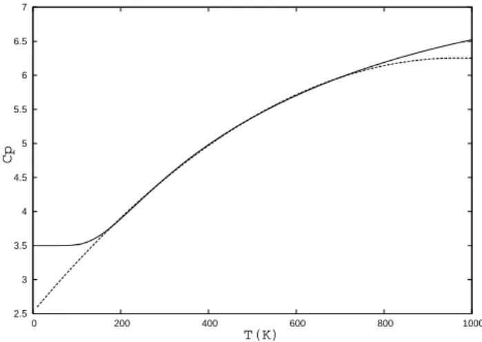
Fig. 1. Specific heat at constant pressure (Cp) in units ofR∗as a
function of temperature (T), of theCO2molecule (continuous line)
and its polynomial fit (dashed line). For details see Sect. 4.
4 Specific heat of CO2
The molecule of CO2is linear and consists of a carbon atom that is doubly bonded to two oxygen atoms. Its molecular mass and corresponding specific gas constant are
MCO2=44.01g mol
−1; R=M CO2×R
∗=188.92 J kg−1K−1. The various contributions to the specific heat, at constant pressure, of a gas constituted by molecules of this type are expressed in the form:
Cp=
7 2R+
X
Tν
R
Tν
2T
2
sinh−2
Tν
2T
. (15)
The first term in this sum corresponds to translation and to rotational modes while the second term is due to vibrational modes. The sum in the second term extends to the various characteristic temperatures,Tν, of the vibrational modes. For
CO2, these values are (Callen, 1980)
Tν(K)=960,960,2000,3380. (16) For practical uses, it is convenient to express Eq. (15) by a simple algebraic approximation. Thus, it is standard to ex-press the specific heat by a series of powers inT, with coef-ficients empirically adjusted. Three terms, namely
Cp=A+B T +C T2, (17)
10-3 10-2 10-1 100 101 102 103 104
200 300 400 500 600 700 800
T(K)
z=0 km
z=100 km
p(kPa)
z=34 km
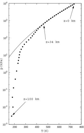
Fig. 2. Pressure-temperature profile of the atmosphere of Venus.
The data (black dots) have been taken from Table 1, and the fitting line is an adiabatic as given by Eq. (19).
Eq. (16). The dotted line is the polynomial approximation (17), the coefficients being
A=2.5223, B=0.77101 10−2, C= −0.3981 10−5.
The units ofA,B andCareR∗,R∗/K andR∗/K2 respec-tively. From Fig. 1 it is apparent, first, thatCphas a
signifi-cant change in the range of temperatures of the Venus atmo-sphere, from 735 K atz=0 to 175 K atz=100 km. Even if we restrict our analysis to the lowest layer, i.e., fromz=0 to
z=40 km, the interval of temperature is between 735 K and 385 K. In Fig. 1 one first observes that the change inCp in
this interval of temperature is of the order of 50%, and sec-ondly, that this polynomial fit is excellent. Thus, we will use Eq. (17) as input to generalize the VG method and apply it to the atmosphere of Venus.
5 Potential temperature for a temperature-dependent specific heat
The generalization of the VG method can start from Eq. (4) because it is applicable to any ideal gas. In this section how-ever, Eq. (5) for the adiabatic transformations, adopts the form
Z T
θ
Cp(T′) δT′
T′ ≡
Z T
θ
(A+B T′+C T′2)δT ′
T′ =R ∗
Z p
pr
δp′ p′.
(18)
pr being the pressure level of reference andθ the potential
temperature characteristic of this adiabatic trajectory. We find
p pr
=
T
θ
A/R∗
exp
B (T−θ )
R∗
exp
"
C (T2−θ2)
2R∗
#
.
(19) In Fig. 2, we have adjusted the data of the low atmosphere of Venus by means of this formula for an adiabatic. There is a generalized consensus supporting this behavior as can be read in ref. Seiff et al. (1980). It shows an excellent agree-ment along the lowest 30 km and a clear departure for upper heights.
In the present case, the physical meaning of the potential temperature is the same as that of Eq. (7), i.e. the temperature that the gas would take if we compressed or expanded it adia-batically to a pressurepr. The price to pay now is that given
the coordinates(p, T ), the value ofθ has to be computed numerically by iterations. Of course, in the caseB=C=0, Eq. (7) and Eq. (19) are the same equation.
The differential expression for the specific entropy of ideal gases was written in Eq. (8) and now reads
δs=Cp(T )δT T −R
∗δp
p . (20)
For practical purposes, let us define a new magnitudeτ, with physical dimensions of temperature, in the following way:
Cp(T ) δT
T =C 0 p
δτ
τ , (21)
with
Cp0=Cp(T0) ; τ (T0)=T0. (22) In fact, this new variableτ,that reduces to the standard tem-perature as soon asCp is constant, allows one to treat this
After specifyingCp(T )in a form like Eq. (17), and by the
integration of Eq. (21) we obtain
Cp0
Z τ
T0 δτ
τ =
Z T
T0
A+B T +C T2 δT
T (23)
=A[ ln
T
T0
+B
A (T −T0)
+ C
2A
T2−T02],
and the result is ln
τ
T0
=A
C0 p
ln
T
T0 exp
B
A (T−T0)+ C
2A
T2−T02
.
(24) This is the relation betweenτ andT. This formula fulfils the two agreed upon conditions:τ (T0)=T0andτ (T )=T for B=C=0
Using Eq. (21) in Eq. (20)
δs=Cp0 δτ τ −
R∗ C0 p
δp p
!
, (25)
and in a similar way to what was done to arrive to Eq. (10), we obtain
s=Cp0 lnτ˜+constant, (26)
with
˜ τ =τ
p
pr
−κ0
, (27)
and
κ0= R
∗
C0 p
. (28)
It is now clear from this result that in an isentropic process,τ˜
is also conserved. The use of Eq. (26) will permit us to extend the VG method quite easily, at least from a conceptual point of view.
6 Generalization of the VG method
The formal analogy between these new magnitudes and those appearing in Sect. 2,τ˜↔θ,κ0↔κ, permits us to extend the VG method reviewed in Sect. 3 in a quite natural way. The entropy, the enthalpy and the L function of an atmospheric column per unit section are:
S=C
0 p g
Z p1
p2
lnτ dp,˜ (29)
H= 1 g
Z p1
p2
h dp= 1 g
Z p1
p2
Cp(T ) T dp, (30)
10-3 10-2 10-1 100 101 102 103 104
200 300 400 500 600 700 800
T(K)
z=0 km
z=100 km
p(kPa)
z=85 km
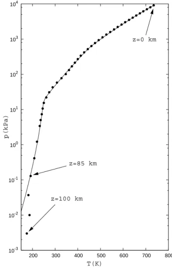
Fig. 3. Pressure-temperature profile of the atmosphere of Venus.
The data (black dots) come from Table 1 and the theoretical re-sults (continuous line) have been obtained using the extended VG method.
L= C
0 p g
Z p1
p2 ˜
τ dp. (31)
The condition of maximumS, with H andLconstants, is expressed as the extreme of the functional9under the vari-ation of the profileT (p), in the following way
δ9=
Z p1
p2 Cp0
g
Z p1
p2 δ
lnτ˜+µτ˜
dp+λ1 g
Z p1
p2
δ[h]dp=0.
(32) To go into the details of this variational problem, remember that
Then, the conditionδ9=0 (pfixed) implies that
1
˜ τ +µ
δτ˜
δT + λ C0
p δh
δT =0, (34)
and taking into account that
T Cp0 δlnτ˜
δT =
δh
δT, (35)
one gets
1
T +µ ˜ τ T
+λ=0. (36)
Finally, the result of the extreme can be written as
T =T0
1+α
1+ατ /T˜ , (37)
with
α= µ
λ ; T0=
1
λ, (38)
being formally identical to the VG result. Nevertheless, it does not provide an explicit expression ofT as a function of
p. This is due to the fact thatτ˜ depends onτ and through it onT, so thatτ /T˜ is now a function ofp andT. Conse-quently, the Eq. (37) has to be treated numerically. In fact, by using the method of Lagrange multipliers, the experimental data fix the constraintsH andL. Then, the parametersT0 andαare determined in order to satisfyHandL.
7 Results of the extended VG method
The performance of the extended VG method, summarized in Eq. (37), when applied to the atmosphere of Venus is shown in Fig. 3. Note that the logarithmic scale used for pressure is more sensitive and hence puts more clearly in evidence the virtues or flaws of the fit. The characteristics of the Venus atmosphere allow us to well distinguish three regions in al-titude. In each one of these regions we have applied the ex-tended VG method by maximizing the entropy with bothH
andLconstraints.
In the lowest one, fromz=0 toz≃34 km, we found that the value ofαis 44 and the value ofT0=735 K. This high value of the unique parameter of the model indicates the clear prepon-derant role ofLwith respect toH, as the dominant constraint in the maximization ofS. From this fact we conclude that in this layer the profile is adiabatic. This clearly agrees with the result shown in Fig. 2, obtained by means of Eq. (19).
In the layer from z≃60 km to z≃100 km, the value ob-tained forαis 0.18 andT0=245 K. This indicates that hereH is the dominant constraint, and in consequence the profile of this layer is basically isothermal.
The method assignsα=3 withT0=444 K to the intermedi-ate layer, a transition region, fromz≃34 km toz≃60 km.
8 Discussion and conclusions
Our purpose in this paper was to extend the first-principles VG method to atmospheric layers where the thermal devia-tion is so high that it is not reasonably possible to consider a constant unique value for the specific heat in all the points of the layer. To implement this extension, we have had to define a new extended potential temperature,τ˜. A potential temperature is, by definition, a generalized temperature that characterizes adiabatic processes, or in other words, that is conserved in processes where the entropy is constant. The relation between the newτ˜ and entropy maintains the same standard form as that existing for ideal-perfect gases.
From the surface of Venus up to about 100 km, we have distinguished 3 layers. The extended VG method, for each layer, after fixingT0to the corresponding initial temperature of the layer, deals with a unique parameterαto adjust the constraints. From the surface up to 35 km, the method as-signs a high value ofα. This implies that thep−T profile here is adiabatic. There is no surprise in this result; an adia-batic lapse-rate was detected in the low atmosphere of Venus during the first observations of the Russian Venera probes. This was verified later in other spatial missions (Seiff et al., 1980). In the layer from 35 to 65 km in heightαhas an in-termediate value that indicates a transition. Finally, from 65 to about 100 km, this method produces a lowα, which is in-terpreted as an isothermal layer. This is the first time that the VG method identifies an adiabatic layer where it should; this concordance shows clearly the success of the method itself and of the extension presented in this paper.
Acknowledgements. L. N. Epele, H. Fanchiotti and C. A. Garc´ıa Canal acknowledge CONICET and ANPCyT of Argentina for financial support. A. F. Pacheco and J. Sa˜nudo thank the Spanish DGICYT for financial support (Project FIS 2005-06237).
Edited by: T. Chang
Reviewed by: two anonymous referees
References
Bohren, C. F. and Albrecht, B. A.: Atmospheric Thermodynamics, Oxford Univ. Press, 1998.
Callen, H. B.: Thermodynamics, John-Wiley and Sons, p. 323–327, 1980.
Landis, G., Colozza, A., and LaMarre, C.: Atmospheric flight on Venus, NASA-2002-0919, 2002.
Pacheco, A. F. and Sa˜nudo, J.: A maximum entropy
pro-file for the mesosphere, Nuovo Cimento, C28, 29–32,
doi:10.1393/ncc/i2005-10021-9, 2005.
Seiff, A., Kirk, D. B., Young, E., et al.: Measurements of Thermal Structure and Thermal Contrasts in the Atmosphere of Venus and Related Dynamical Observations: Results from the Four Pionner Venus Probes, J. Geophys. Res., 85, 7903–7933, 1980.
Tsonis, A. A.: An Introduction to Atmospheric Thermodynamics, Cambridge Univ. Press, 2002.