Using Real-World Car Traffic Dataset in Vehicular Ad Hoc Network Performance Evaluation

(1)

Using Real-World Car Traffic Dataset in Vehicular

Ad Hoc Network Performance Evaluation

Lucas Rivoirard

Univ Lille Nord de France, IFSTTAR, COSYS, LEOST F-59650 Villeneuve d’Ascq, France

Marion Berbineau

Univ Lille Nord de France, IFSTTAR, COSYS

F-59650 Villeneuve d’Ascq, France

Martine Wahl

Univ Lille Nord de France, IFSTTAR, COSYS, LEOST F-59650 Villeneuve d’Ascq, France

Dominique Gruyer

IFSTTAR, COSYS, LIVIC F-78000 Versailles, France

Patrick Sondi

Univ. Littoral Cˆote d’Opale, LISIC - EA 4491 F-62228 Calais, France

Abstract—Vehicular ad hoc networking is an emerging paradigm which is gaining much interest with the development of new topics such as the connected vehicle, the autonomous vehicle, and also new high-speed mobile communication technologies such as 802.11p and LTE-D. This paper presents a brief review of different mobility models used for evaluating performance of routing protocols and applications designed for vehicular ad hoc networks. Particularly, it describes how accurate mobility traces can be built from a real-world car traffic dataset that embeds the main characteristics affecting vehicle-to-vehicle communications. An effective use of the proposed mobility models is illustrated in various road traffic conditions involving communicating vehicles equipped with 802.11p. This study shows that such dataset actually contains additional information that cannot completely be obtained with other analytical or simulated mobility models, while impacting the results of performance evaluation in vehicular ad hoc networks.

Keywords—MOCoPo dataset; mobility models; vehicular ad hoc networks; simulation; performance evaluation

I. INTRODUCTION

VANET (Vehicular Ad Hoc Network) is a promising ap-plication of MANET (Mobile Ad Hoc Networks) where nodes consist of vehicles which organize themselves in order to communicate efficiently. Using ad hoc communications allow fast and direct vehicle-to-vehicle (V2V) exchanges, besides the telecommunication services that can be offered by an infrastructure, when it exists, through vehicle-to-infrastructure communications (V2I). For instance, vehicles can exchange contextual or traffic management information. Safety and se-curity applications can also rely on V2V communications in order to avoid a collision or send post-crash warnings.

With the wide deployment of 3G and 4G infrastructures, many new mobile services are proposed to drivers through their smartphones or built-in car devices. Both the network service providers and the designers of these applications can make use of the information collected over thousands of users in order to evaluate and to improve the performance. Such opportunity is not yet accessible to vehicular ad hoc networks due to nonexistence of large-scale experimentation. Also, V2V applications will not be widely adopted unless serious studies

and evaluations prove their efficiency in realistic car traffic contexts. Consequently, building accurate testing environments for VANET performance evaluation is a crucial issue for the future of V2V communications. The performance of VANETs can be evaluated by means of real-world testings on the ground or through modelling and simulation. For the aforementioned reasons, the first solution may be costly and will not carry out the whole field situations: it is difficult to equip a significant number of vehicles and to experiment the performance of network communication in every different traffic conditions. The second solution, namely modelling, is easier to realize by means of computers and may include many complex models. However, the accuracy depends notably on the availability of realistic mobility models.

The authors of [1] and [2] show that, depending on the mobility model, the results of performance evaluation are different for the same routing protocol. An example is developed in [1] based on the DSR protocol. Generally in the literature, the modelling of vehicle mobility are made thanks to random patterns, microscopic traffic simulators, or real traces of vehicles. In this paper, the authors discuss the benefit of using real traces of vehicles extracted from car traffic dataset in simulation-based evaluation of vehicular ad hoc network performance. This study uses the real traces processed by [3] based on road videos filmed by helicopter within the context of the French research project named MOCoPo (Measuring and Modelling Congestion and Pollution).

The paper is organized as follows. First, some work related to mobility models in vehicular ad hoc network are presented. The MOCoPo dataset traces are described, and then discussed in comparison with other mobility models. A simulation sys-tem is configured in order to realize performance evaluation of a VANET using the proposed dataset. Finally, the simulation results are discussed, before the conclusion.

II. RELATEDWORK

(2)

evolution, notably the historical Random Waypoint, the Man-hattan model, the microscopic traffic simulators, and finally the real traces from car traffic dataset.

A. Random Waypoint model

The first mobility model used in VANET studies was the Random Waypoint model (RW). In this model, each node randomly chooses an origin and a destination in the simulation representation of the space, and also a speed value between zero and a given maximum limit. The speed remains fixed along the journey. Once the destination is reached, a timer is triggered, and the node selects a new destination and a new speed value.

This model, very simple to set up, is still used in many studies such as [8]–[11]. It is often used for VANET because it allows to define high speed nodes. In fact in most European countries, under normal conditions, a vehicle in a VANET can travel up to 130 km/h on the highway. Therefore, the relative speed between two vehicles can vary from 0 to 260 km/h.

However, the path followed by the nodes in RW model is always a straight line. Moreover, it does not take into account the restricted vehicle motion degrees imposed by the road layout. Last, the significant dispersion of the speed values over the time and space is also another important feature of mobility that cannot be taken into account with this model. Indeed, during its journey, vehicle speed on highway can be either 130 km/h in a fluid traffic or 5 km/h in case of congestion [12]–[14].

B. Manhattan model

The Manhattan model improves the Random Waypoint model by introducing a representation of the vehicle motion degrees. The nodes move on a road represented by a grid that limits the vehicle movement. Origins and destinations of the vehicle trajectories are randomly chosen. The trajectories are calculated either by algorithms such as the Dijkstra shortest path or by using a probability to select a direction when vehicles arrived at a cross-road. The Manhattan model is used for instance in [15] or [16].

However, in real life, road users must respect the traffic rules and sign regulations; vehicles are constantly reacting according to each other. This cannot be observed in the Manhattan model where vehicles can move across each other.

C. Microscopic traffic simulator

Various studies, related to traffic theories [12]–[14], [17], [18], strive to model driver behaviour. The models are realized through microscopic simulators which implement one of the following models : stochastic models, traffic flow models, car following models, queue models, or behaviour models. They simulate every car in detail, with breaks, accelerations and lane changing. Such simulators bring a road representation that the random mobility model does not, and they implement the significant dispersion of speed values over time and space. They easily allow researchers to schedule a mobility scenario such as a congested highway. Among them, SUMO [19] and VanetMobiSim [20] are the most referenced in the literature (for instance [21], [22]). They take into account multi-lane

roads, vehicles changing lane, speed limits, and intersection priorities (stop signs and traffic lights) [7].

Nevertheless, the choice of the origin and destination for a vehicle is randomly selected whatever the road reality. An-other drawback is that microscopic simulators use probability profiles like acceleration or deceleration profiles which add a difference between the model and the reality. This is especially true for extreme driving behaviours which are not considered.

D. Real traces of vehicles

Mobility traces of vehicles through GPS data can be easily found nowadays. As an example, the Community Resource for Archiving Wireless Data At Dartmouth (CRAWDAD, [23]) provides trajectory datasets for VANET studies. GPS traces are obtained with map-matching algorithms. They come from specific vehicle fleets, such as bus or taxi fleets, which sometimes travel with dedicated work constraints. They do not come from common car users which are the first user class of road.

Real traces based on GPS can be used to study the connection time between vehicles. In this way, [24] uses GPS traces from taxis and shows that the high mobility of VANETs induces time-limited connections between vehicles. Indeed, two vehicles, travelling from opposite directions on the highway at 130 km/h and having a maximum communication range of 500-meter long, will only communicate for up to 15 s [25]. In fact, a difficulty of using GPS real traces is that, currently, either vehicles are not close together (dis-persed within a wide area) or they include very few vehicles. Consequently, such traces do not allow an accurate study of V2V ad hoc communications with various vehicle density. However, the traces provided by CRAWDAD could be relevant to study the procotocols and applications relying on vehicle-to-infrastructure communications.

It is possible to obtain real traces of vehicle trajectories with aerial road traffic recordings. Studies had been achieved in the past by mounting a camera on a fixed position or on-board aerial platform [26]. [3] notes that two main groups of datasets were constructed since the beginning of this century: series of datasets resulting from the experiments conducted in the Netherlands by the TU Delft [27] and the datasets of the NGSim project, conducted with the funding and supervision of FHWA [28]. Only the NGSim datasets are made publicly available on the web. But there is noise in the longitudinal and lateral positional information of vehicles, and data need to be filtered in order to determine their positions, velocities, and accelerations [29].

III. A CARTRAFFICDATASET FORVANETEVALUATION

A. Presentation of the MOCoPo data

(3)

data were collected. The site of the project [30] provides maps and access to the data.

Fig. 1. The 500-meter-long RN87 section filmed in Grenoble southern suburb. The insertion lane is in green, the right lane in red, and the fast lane in blue.

Collected data are from a 500-meter-long express road with a speed limit of 70 km/h. For this area, data collection periods were chosen to cover the congestion occurring in morning rush hours.

In order to be transformed into trajectories, the MOCoPo videos were processed. Firstly, as the helicopter was not perfectly fixed, the MOCoPo research teams corrected the curvature of the image and stabilized the image. They also reframed the images to focus on a region of interest containing only the road. Secondly, a reference image was used to extract moving objects from all images of the video on the region of interest. This image was a photography of the infrastructure without any vehicle. They connected the different objects in order to build the trajectory of each vehicle. Thirdly, [3] implemented a new filtering approach based on polynomial fitting and the polar coordinates. The method was developed in two versions: wise constant accelerations or piece-wise linear accelerations. [3] shows that their process provides values of acceleration fully compatible with the physical limits of vehicles found in the literature. Thus, there is no need to add extra constraints to the data such as a limitation for acceleration or deceleration.

As a result, [3] supplies a set of trajectory data from video recording of 16th September 2011 (between 7:58 and 8:58 am). This set is composed of a sample of 619 vehicles distributed in a 60-minute time window. Each trajectory consists of a sequence of location data provided every 0.1 s.

B. MOCoPo trajectory interest for VANETs

Getting real-world traces usable for VANETs studies is not obvious. GPS-trace databases concern vehicles geographically dispersed or few vehicles; NGSim datasets need to be pro-cessed in order to obtain the final usable trajectories.

The MOCoPo database consists of vehicles close to each other recorded during rush hours. Its data contain the in-formation on the driver behaviours (speed, acceleration, lane changing...). Moreover, the data show periods of congestion where vehicles stop and restart after a few moments (so-called stop and go wave) and where vehicle speeds are highly variable. It is therefore interesting to find time periods in the database where vehicles have high speed or respectively low speed.

C. Mobility profiles in MOCoPo data

The authors split the trajectory database of MOCoPo into groups corresponding to different congestion scenarios characterised by the speed of the vehicles. The result is shown

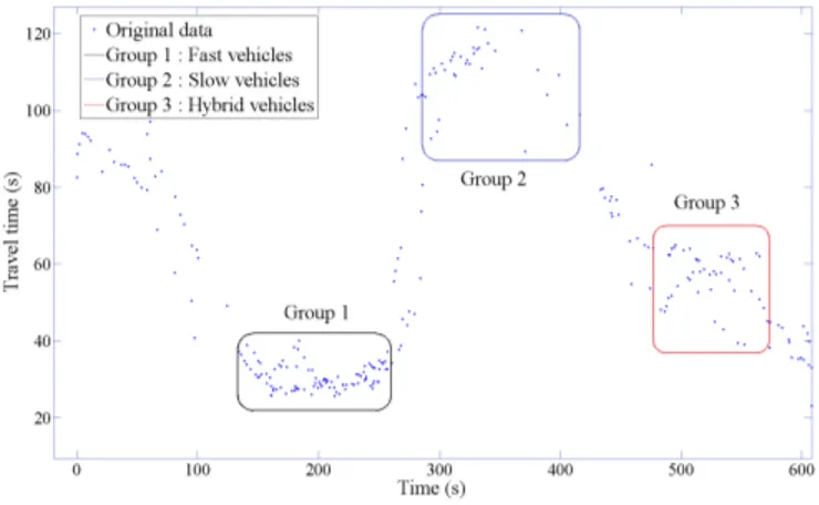
Fig. 2. Travel time of vehicles versus time. Travel times range from 30 to 120 s. Three groups are defined with fast, slow and hybrid vehicle speed.

in figure 2. A significant variation in travel time is observed over time. Some vehicles pass through the area in less than 30 s, i.e with an average speed of 60 km/h, others in more than 120 s, i.e.with an average speed below 15 km/h.

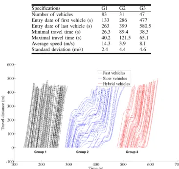
In light of these results, it is relevant to define three groups of vehicles with different mobility features presented in table I. Figure 3 shows the travel distance versus the time for each three mobility groups. The slope of the curve representing each vehicle corresponds to their instantaneous speed. As it can be seen in the figure, the vehicles of group 1 maintain a high speed while the vehicles of group 2 suffer a period of stop and go wave (the slopes of the travel distance curve is horizontal, which means a zero speed). Vehicles of group 3 that are located on the right lane experiment a stop and go wave while those located on the left lane have higher speed. Figure 4 represents the speed distribution experienced by the vehicles in each group.

The three groups are built as follows.

Group 1: 83 vehicles have a short travel time ranging from 26.3 s to 40.2 s. Their date of entry into the area is between 133 s and 263 s. The average speed of this group is 51.3 km/h with a standard deviation of 8.5 km/h. This group is not constrained by stop and wave events. The traffic is dense, but it remains fluid.

Group 2: 31 vehicles have a longer travel time ranging from 89.4 s to 121.5 s. Their date of entry into the area is between 286 s and 399 s. The average speed is 14.28 km/h with a standard deviation of 16 km/h. All vehicles have both stop and wave effects. The traffic is congested.

(4)

TABLE I. CHARACTERISTICS OF THETHREEMOBILITYFEATURE GROUPS

Specifications G1 G2 G3

Number of vehicles 83 31 47 Entry date of first vehicle (s) 133 286 477 Entry date of last vehicle (s) 263 399 580.5 Minimal travel time (s) 26.3 89.4 38.3 Maximal travel time (s) 40.2 121.5 65.1 Average speed (m/s) 14.3 3.9 8.1 Standard deviation (m/s) 2.4 4.4 4.6

Fig. 3. Travel Distance versus time for each vehicle group. Vehicle travel times of Group 1 are below 40 s; the ones of Group 2 are greater than 90 s; Group 3 is an hybrid group with slow and speed vehicles. Stop and go wave occurs in Group 2 and 3 and spreads out from one vehicle to another.

Fig. 4. Speed distribution of vehicles in each group. Distributions correspond to the experienced speed by the group vehicles at each time step (0.1 seconds)

IV. BUILDINGMOBILITYMODELS USINGMOCOPO DATA

In this paper, MOCoPo datasets are taken as a reference. Different mobility models were built by degrading the knowl-edge of the road traffic from the MOCoPo data (figure 5). The resulting models and trajectories are explained in this section.

A. MOCoPo data

The MOCoPo data consist of the positions of the vehicles provided every 0.1 second (see section III-B).

B. GPS-based model - Fixed speed

The GPS-based model, called fixed speed, is based on the knowledge of vehicle positions in the MOCoPo data, but by

Fig. 5. Different mobility models according to the knowledge of the road traffic. (left) Real data extracted from MOCoPo data, (center) Fixed speed model with a position extracted everyδsecond from MOCoPo data, (right) SUMO simulation calibrated with travel times of vehicle as if coming from the knowledge of the departure and arrival time measured with electromagnetic loop detectors and merged with an identification system.

keeping a weaker refresh rate than 0.1 second. These data are built as if they were provided by vehicle GPS systems. The positions that each vehicle has every δ seconds are extracted from the MOCoPo data. Nodes are then forced to have these intermediate collected positions. Since the construction of this model assumes only the position of the vehicles at δ -second interval, fixed speeds are taken between two positions. Therefore, the node speed is given by the ratio between the travel distance and the δ-second interval. The chosenδ are : 0.5, 1, 3, 5 and 10. Each δ-second fixed speed trajectory is therefore designed as a set of segments meeting the original MOCoPo trajectory curve every five positions forδ= 0.5, ten positions for δ= 1, thirty positions for δ= 3, fifty positions for δ = 5, and hundred positions for δ = 10. The highest refresh rate has been set atδ= 10seconds since some vehicles have a travel time inferior to 30 seconds.

C. Detector-based model - SUMO simulation

The detector-based model only keeps the knowledge of the departure and arrival times of the vehicles extracted from the MOCoPo data. The data used are then similar to the outputs of a system composed of two electromagnetic loop detectors and a vehicle identification system (such as an automatic number plate recognition, a camera, or a bluetooth system). The trajectories of vehicles are still to be built from these departure and arrival times. The SUMO microscopic traffic simulator software has been chosen to simulate the behaviour of the vehicles and create the trajectories.

A 500-meter-long two-lane road is represented under SUMO with a RN87-like curvature. The parameters of vehicle length is set to 5 meters and the speed limit is set to 70 km/h which corresponds to the legal speed limit on this road.

The default car following models included in SUMO simulator is a modification of Krauß model [31]. The model is simple : each vehicle drives up to its “desired speed”, while maintaining a perfect distance safety with the leader vehicle (i.e. the vehicle in front of it).

To calibrate the model according to the MOCoPo traffic groups, a set of parameters have to be defined for each one.

(5)

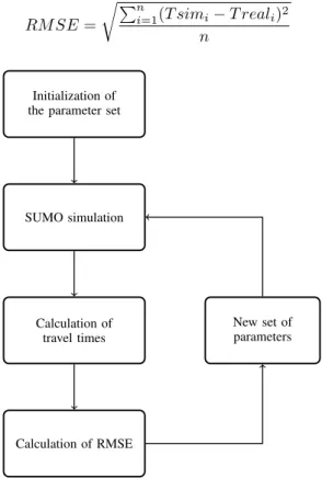
At the initialisation, a first random set of parameters is chosen and the simulation is launched using the real departure dates of vehicles in the MOCoPo data. The SUMO computed arrival dates of vehicles (called T simi for vehicle i) are then compared with the MOCoPo arrival dates of vehicles (called

T reali). Another random set of parameters is drawn for a new simulation run. This method is carried out 500 times for each group of vehicles. Figure 6 sketches the method. The formula used to calculate the gap between the simulation and MOCoPo travel time is :

RM SE= r Pn

i=1(T simi−T reali)2

n

Initialization of the parameter set

SUMO simulation

Calculation of travel times

New set of parameters

Calculation of RMSE

Fig. 6. Method for calibrating MOCoPo data according to travel times

The different parameters to calibrate the car following model are :

• Accel: the acceleration ability of vehicles[m/s2_] • Decel: the deceleration ability of vehicles[m/s2_] • Sigma: the driver imperfection (between 0 and 1)

• Tau: the driver’s desired minimum time headway[s]

• MinGap: the offset to the leading vehicle when stand-ing in a jam [m].

Moreover, to achieve realistic car following behaviour, it is necessary to use speed distributions for the desired speed. Otherwise, if all vehicles have the same desired speed, they will not be able to catch up with their leader vehicle causing unrealistic situation. Therefore, two other parameters have to be calibrated to use speed distributions in SUMO: speedFactor and speedDev. For instance, using speedF actor = 1 and

speedDev= 0.1will result in a speed distribution where 95% of the vehicles drive at a speed ranging from 80% to 120% of the legal speed limit. The results of the calibration for each

group of mobility are presented in table II. The parameters inherent to car following model are relatively close to each other for the three mobility groups. However, the speedFactor parameter is specific to a mobility group.

TABLE II. MODELMOBILITYPARAMETERS WITHIN THESUMO FRAMEWORK

Parameters Interval Group 1 Group 2 Group 3 Accel[m/s2_] _[1:3] _2.28 _2.19 _1.2

Decel[m/s2_] _[1:3] _1.98 _1.99 _2.62

SpeedFactor [0:1] 0.87 0.256 0.61 SpeedDev [0.05:0.15] 0.058 0.065 0.054

Sigma [0:1] 0.22 0.14 0.8

Tau[s] [1:3] 1.8 1.47 1.87

MinGap[m] [5:30] 7.7 7.27 7.5

RMSE[s] - 3.8 8.23 8.72

D. Resulting trajectories

Figure 7 shows positions (graph a) and speeds (graph b) of node 40, taken as an example among the vehicles of group 1. Each curve represents the position (respectively the speed) of node 40 for each one of the mobility models presented. According to the positions, it can be observed that both the 0.5-second and 1-second fixed speed trajectories follow the MOCoPo curve, while the 3-second, 5-second and 10-second ones make the vehicle move away from the lane (near the arrival date). The trajectory simulated by SUMO leads to lane changing: node 40 starts on the left lane, then changes at coordinate X=330 m. The speed values presented in the curves (b) have been computed from the successive positions from the curves (a). The speed curves are piece-wise constant as a function of the sample time related to the positions.

0 50 100 150 200 250 300 350 400 450 −50

−40 −30 −20 −10

X (m)

Y (m)

(a)

Original data Fixed speed 0.5s Fixed speed 1s Fixed speed 3s Fixed speed 5s Fixed speed 10s SUMO 1

320 340 360 380 400 420 −46

−45 −44 −43 −42 −41

X (m)

Y (m)

205 210 215 220 225 230

13.5 14 14.5 15 15.5 16

Time (s)

Speed (m/s)

(b)

Fig. 7. (a) Position and (b) speed of node 40 group 1, over time for the different models of mobility

Figure 8 shows positions (graph a) and speeds (graph b) of node 10, taken as an example for the group 2, for the different mobility models.

Figure 9 shows positions (graph a) and speeds (graph b) of node 3, taken as an example for the group 3, for the different mobility models.

E. Comparison of the resulting trajectories

(6)

0 50 100 150 200 250 300 350 400 450 500 −40

−30 −20 −10

X (m)

Y (m)

(a)

320 340 360 380 400 420 −47

−46 −45 −44 −43 −42

X (m)

Y (m)

320 330 340 350 360 370 380 390 400 410 420 0

5 10 15

Time (s)

Speed (m/s)

(b)

50 100 150 200 250 300 350 400 450 500 −50

−40 −30 −20 −10

X (m)

Y (m)

(a)

320 340 360 380 400 420 −50

−49 −48 −47 −46

X (m)

Y (m)

490 495 500 505 510 515 520 525 530 535 7

8 9 10 11 12

Time (s)

Speed (m/s)

(b)

the speed profile obtained through SUMO simulation tends to be very smooth when compared to the original MOCoPo data. When considering the different approximations of this latter, namely the Fixed speed 0.5, 1, 3, 5 and 10, the curves show that they tend to get closer to SUMO curves as they are less precise in comparison with the original MOCoPo. This means that the simulated trajectory obtained through SUMO using the parameters that reproduce a specific traffic condition may result in a faithful trajectory in terms of positions while not offering any guarantee on the speed profile of the vehicles. Consequently, though simulated trajectories from SUMO could be useful for global simulation requiring realistic vehicle trajectories on the roads, the specific studies that investigate the performance in realistic traffic conditions, especially when the speed profile is important, should better rely on real-world traces such as car traffic dataset. Even when considering only few points of the original trajectory, in order to reduce the amount of data necessary to reproduce the trajectory in the simulation, one can observe that the resulting approximative curves (Fixed speed 0.5, 1, 3, 5 and 10) remain closer to the original traces when compared to SUMO trajectory. This is particularly clear when considering group 2 and group 3 which are the most concerned with speed variations due to congestion in their traffic.

Figure 10 shows the average speed of the vehicles for the

three mobility groups. As for the individual vehicles presented in figures 7, 8, 9, the average values on every vehicles in each group confirm that the speed profile obtained with SUMO is too smooth in comparison with the real traces, especially in group 2 and group 3.

140 160 180 200 220 240 260 280 0

10 20

Speed (m/s)

Time (s)

Group 1

300 350 400 450 500 550

0 10 20 30

Speed (m/s)

Time (s)

Group 2

480 500 520 540 560 580 600 620 10

20 30

Speed (m/s)

Time (s)

Group 3

Number of vehicles at time t Average speed Average speed + σ Average speed − σ SUMO Speed of sample vehicle

Fig. 10. Average speed of the vehicles in the network over time for group 1, 2 and 3 in the case of the MOCoPo (blue curves) and SUMO (red curves) models. The speed of MOCoPo vehicles number 40, 10 and 3 respectively taken as an example in group 1, 2 and 3 (green curves). Number of vehicles present in the network over time (black curves)

V. SIMULATIONDESCRIPTION ANDRESULTS

The purpose is to evaluate the impact of the differences in the speed profiles of the mobility models (the position traces are almost the same for all) on network performance through simulation results. The results obtained with original MOCoPo dataset traces are compared with those obtained using two other mobility models (fixed speed and SUMO) regarding the three groups of mobility (group 1, group 2, and group 3).

These simulations rely on the ability of Riverbed OPNET Modeler software to assign a trajectory to each node of a communication network by means of external TRJ files in the OPNET format. The following paragraphs present the simulation system configuration and the application. Then, the results are discussed.

A. Simulation system configuration

The simulated system is an ad hoc network formed with IEEE 802.11p nodes that use the proactive OLSR protocol as the routing protocol (Optimized Link State Routing Protocol [32]). IEEE 802.11p is an amendment of the IEEE 802.11 standard of 2012. Created to answer the challenges imposed by ad hoc vehicular networks [14], it applies in the frequency band of 5.9 GHz for wireless access in a vehicular environ-ment (WAVE - Wireless Access in Vehicular Environenviron-ment). IEEE 802.11p considers dedicated short range communication (DSCR). The implementation of IEEE 802.11p used is the one proposed with the OPNET modeler suite, and the chosen node configuration is summarized in table III.

(7)

TABLE III. NODECONFIGURATION

Attribute Value

Physical Characteristics 5.0 GHz Data Rate 13 Mb/s Transmit power 0.001 W Receiver sensitivity -95 dBm Transmission range 225 m Packet length 75 bytes Frequency of sending 40 Hz Transport protocol UDP Response packets 0 byte

TABLE IV. ROUTINGPROTOCOLCONFIGURATION

Routing protocols Value Hello interval 2 s

TC interval 2 s

Neighbour hold time 6 s Topology hold time 15 s Duplicate message hold time 30 s

each known destination. Moreover, OLSR tries to reduce the impact of flooding due to broadcast traffic by selecting a subset of special nodes called the multipoint relays (MPR) which are the only allowed to retransmit broadcast traffic in the entire ad hoc network. This latter reason makes it a good choice as the routing protocol for the evaluations performed in this paper since the dataset contains dense VANETs [33] in addition to the fact that a built-in implementation of OLSR is proposed in the OPNET modeler suite.

B. Application

A data traffic model for VANET studies is defined in [34] . The IEEE settings correspond to a 300-byte packet length sent with a 10-Hertz update rate. The authors are especially interested in future real time VANET application such as for autonomous cars. In such safety applications, on-board functions (sensor functions, geo-localization, extended perception, etc.) will have to share variables periodically (speed, acceleration, positioning information, etc.) for their inner process.

The deployed application in this paper consists in a trans-mission of a message from a source vehicle to all other vehicles in the network. This application may represent, for example, a safety alert in case of accident. However, to operate really like a real-time application, a higher exchange frequency than IEEE setting is needed. Keeping the same total amount of exchanged data, so the same throughput than IEEE setting, a node will send 75-byte packets every 25 ms. The sender node is selected for each mobility group, respectively the node 40, 10 and 3 for the group 1, 2 and 3. The trajectories of theses particular vehicles are shown in figure 7, 8, 9.

C. Performance metrics

The three following performance metrics are considered:

• The “load” metric represents the total number of bits forwarded from the wireless layer to higher layers. This metric measures the traffic received in all the network at a given time.

• The “throughput” metric represents the total number of bits submitted to wireless layer by all higher layers. Its upper value is restricted by the bandwidth, so it

may give an idea of the local bandwidth obtained by each node with each mobility profile.

• The “end-to-end delay” metric concerns the time taken by a packet to reach the wireless layer of the receivers. It is measured as the difference between the arrival time of a packet at its destination and the creation time of this packet. This metric will help to evaluate the network performance in relation to the application requirements.

D. Scenarios and results

Each scenario is run several times with different seed values for the random generator in order to avoid that the related sequence favors one of the scenarios.

Figures 11 to 13 present the average results for each performance metric.

205 210 215 220 225 230 235 0

5 10 15x 10

5

Time (s)

Load (bit/s)

Group 1

MOCoPo Fixed speed δ=1s Fixed speed δ=10s SUMO

320 340 360 380 400 420 440 0

5 10

x 105

Time (s)

Load (bit/s)

Group 2

490 500 510 520 530 540

0 5 10

x 105

Time (s)

Load (bit/s)

Group 3

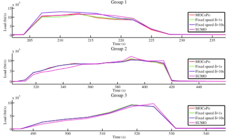
Fig. 11. Load for each mobility group with different mobility models

140 160 180 200 220 240 260 280 300 320 0

5 10 15x 10

5

Time (s)

Throughput (bit/s)

Group 1

300 320 340 360 380 400 420 440 460 480 500 0

5 10 15x 10

5

Time (s)

Throughput (bit/s)

Group 2

480 500 520 540 560 580 600 620 640 660 0

5 10

x 105

Time (s)

Throughput (bit/s)

Group 3

Fig. 12. Throughput for each mobility group with different mobility models

(8)

205 210 215 220 225 230 235 240 0

0.2 0.4 0.6

Time (s)

Delay (s)

Group 1

380 390 400 410 420 430

0 0.2 0.4 0.6

Time (s)

Delay (s)

Group 2

505 510 515 520 525 530 535

0 0.05 0.1 0.15 0.2

Time (s)

Delay (s)

Group 3

Fig. 13. Delay for each mobility group with different mobility models

TABLE V. MEAN OFGAP BETWEENMOCOPO ANDOTHERMOBILITY MODELSRESULTS

Mobility Group 1 Group2 Group 3

models L T D L T D L T D

FSδ= 0.5 8.3 3.3 11.7 4.6 16.0 4.2 1.8 9.8 0.2 FSδ= 1 8.9 4.5 14.7 5 17.5 5.2 0.8 16 0.1 FSδ= 3 9.2 4.2 13.7 9.4 23.3 6.7 2.3 21.2 0.1 FSδ= 5 14.6 7.1 15.3 8.3 22.6 13 2.4 41.3 0.7 FSδ= 10 20.6 12.8 20.8 5.4 46.3 16.5 5.6 81.2 1.9 SUMO 12.5 5.6 28.4 27.1 117.3 30.7 17.2 92.6 9.2

FS : fixed speed, L : load (kbit/s), T : throughput (kit/s), D : delay (s)

VI. CONCLUSION

The development of big data announces the availability of many datasets including vehicle trajectories in smart city. Targeting a future generalization of such data in the evaluation of vehicular networks, this paper demonstrates the use of the MoCoPo dataset which includes the real-world traces of the cars in a road section.

Though they were early acquired for studies in the domain of road traffic theory, one of the goals of this paper was to show that the MOCoPo data particularly fit to the evaluation of vehicular ad hoc networks in comparison with other mobility models such as those coming traffic simulators. After they have been split into three groups corresponding to different mobility profiles namely fluid (group 1) hybrid (group 2) and congested (group 3) traffics, the MOCoPo dataset traces have been used to simulate the scenarios of a group of communicating vehicles. Other mobility models have been used for the same scenarios in order to compare the behaviour of the system in both cases. The results demonstrate the importance of the granularity of the traces which affects the topology of the road traffic and therefore the communications.

Moreover, the real speed variations embedded in the Mo-CoPo trajectories cannot be reproduced using traffic simulator through basic parameters. The analyzed figures show that even if the position traces, average speed and acceleration threshold are the same, the instantaneous speed of the vehicles in real-world traces are never reproduced by traffic simulators which tend to smooth the speed profile according to the average speed. Therefore, the difference in the speed profiles has an impact on the results obtained through simulation for several performance metrics such as the load, the throughput and significantly the delay.

This work suggests that it is crucial to get real-world trajectory data with refined granularity in order to obtain, through simulation, a performance of vehicule-to-vehicule communication that reflects better the reality in comparison with other mobility models.

ACKNOWLEDGMENT

The authors gratefully thank Dr. Christine BUISSON, researcher in traffic theory at IFSTTAR, for her crucial role in the acquisition of the MOCoPo dataset and for allowing to use it. They acknowledge the support of the CPER ELSAT 2020, the Hauts-de-France region, and the European Community.

REFERENCES

[1] T. Camp, J. Boleng, and V. Davies, “A survey of mobility models for ad hoc network research,” Wireless Communications and Mobile Computing, vol. 2, no. 5, pp. 483–502, 2002.

[2] A. Mahajan, Urban mobility models for vehicular ad hoc networks. phdthesis, Florida State University, 2006. http://diginole.lib.fsu.edu/ islandora/object/fsu%3A181041.

[3] C. Buisson, D. Villegas, and L. Rivoirard, “Using Polar Coordinates to Filter Trajectories Data without Adding Extra Physical Constraints,” in Transportation Research Board 95th Annual Meeting, vol. 16, Transportation Research Board, 2016.

[4] P. Manzoni, M. Fiore, S. Uppoor, F. J. M. Dom´ınguez, C. T. Calafate, and J. C. C. Escriba, “Mobility Models for Vehicular Communications,” in Vehicular ad hoc Networks, pp. 309–333, Springer International Publishing, 2015.

[5] J. Harri, F. Filali, and C. Bonnet, “Mobility models for vehicular ad hoc networks: a survey and taxonomy,”IEEE Communications Surveys Tutorials, vol. 11, no. 4, pp. 19–41, 2009.

[6] C. Sommer and F. Dressler, “Progressing toward realistic mobility models in VANET simulations,” IEEE Communications Magazine, vol. 46, pp. 132–137, Nov. 2008.

[7] H. Hartenstein and K. Laberteaux,VANET: vehicular applications and inter-networking technologies, vol. 1. Wiley Online Library, 2010. [8] N. Garg and P. Rani, “An improved AODV routing protocol for

VANET (Vehicular Ad-hoc Network),”International Journal of Science, Engineering and Technology Research (IJSETR), vol. 4, no. 16, p. 1024, 2015.

[9] A. Roy, B. Paul, and S. K. Paul, “VANET topology based routing protocols & performance of AODV, DSR routing protocols in random waypoint scenarios,” pp. 50–53, 2015.

[10] S. Mohapatra and P. Kanungo, “Performance analysis of AODV, DSR, OLSR and DSDV Routing Protocols using NS2 Simulator,”Procedia Engineering, vol. 30, pp. 69 – 76, 2012.

[11] D. Tian, Y. Wang, G. Lu, and G. Yu, “A vanets routing algorithm based on euclidean distance clustering,”2nd International Conference on Future Computer and Communication (ICFCC), vol. 1, pp. V1–183, 2010.

[12] F. D. d. Cunha, A. Boukerche, L. Villas, A. C. Viana, and A. A. F. Loureiro, “Data Communication in VANETs: A Survey, Challenges and Applications,” report RR-8498, INRIA Saclay ; INRIA, Mar. 2014. [13] J. Jakubiak and Y. Koucheryavy, “State of the Art and Research

Challenges for VANETs,” in the 5th Conference IEEE Consumer Communications and Networking (CCNC ’08), pp. 912–916, Jan. 2008. [14] S. Al-Sultan, M. M. Al-Doori, A. H. Al-Bayatti, and H. Zedan, “A comprehensive survey on vehicular Ad Hoc network,” Journal of Network and Computer Applications, vol. 37, pp. 380–392, 2014. [15] G. He, “Destination-sequenced distance vector (DSDV) protocol,”

tech-nical report, 2002. Networking Laboratory, Helsinki University of Technology.

(9)

[17] S. Xi and X.-M. Li, “Study of the Feasibility of VANET and its Routing Protocols,” in 4th International Conference on Wireless Communica-tions, Networking and Mobile Computing, 2008. WiCOM ’08, pp. 1–4, Oct. 2008.

[18] I. B. Jemaa, Multicast Communications for Cooperative Vehicular Systems. phdthesis, Mines ParisTech, 2014. https://hal.inria.fr/ tel-01101679/document.

[19] SUMO, “Simulation of Urban MObility.” http://sumo.dlr.de/wiki/Main Page. [Online; accessed on November 28, 2016].

[20] VanetMobiSim, “Vanet Mobility Simulation Environment.” http://vanet. eurecom.fr/. [Online; accessed on November 28, 2016].

[21] R. S. Shukla, N. Tyagi, A. Gupta, and K. K. Dubey, “A new position based routing algorithm for vehicular ad hoc networks,” Telecommuni-cation Systems, Dec. 2015.

[22] K. C. Lee, P.-C. Cheng, and M. Gerla, “GeoCross: A geographic routing protocol in the presence of loops in urban scenarios,” Journal on Ad Hoc Networks, vol. 8, pp. 474–488, July 2010.

[23] CRAWDAD, “A Community Resource for Archiving Wireless Data At Dartmouth.” http://www.crawdad.org/. [Online; accessed on November 28, 2016].

[24] Y. Li, D. Jin, Z. Wang, L. Zeng, and S. Chen, “Exponential and Power Law Distribution of Contact Duration in Urban Vehicular Ad Hoc Networks,”IEEE Signal Processing Letters, vol. 20, pp. 110–113, Jan. 2013.

[25] S. Demmel, A. Lambert, D. Gruyer, A. Rakotonirainy, and E. Monacelli, “Empirical IEEE 802.11 p performance evaluation on test tracks,” Intelligent Vehicles Symposium (IV), ’12 IEEE, pp. 837–842, 2012. [26] M. Rafati Fard, A. Shariat Mohaymany, and M. Shahri, “A new

methodology for vehicle trajectory reconstruction based on wavelet analysis,” Transportation Research Part C: Emerging Technologies, vol. 74, pp. 150–167, Jan. 2017.

[27] S. P. V. Z. Hoogendoorn, H. J. , M. Schreuder, B. Gorte, and G. Vosselman, “Microscopic traffic data collection by remote sens-ing,”Transportation Research Record: Journal of the Transportation Research Board, no. 1855, 2003.

[28] FHWA, “Traffic Analysis Tools: Next Generation Simulation (NGSIM).” http://ops.fhwa.dot.gov/trafficanalysistools/ngsim.htm. [Online; accessed on November 28, 2016].

[29] C. Thiemann, M. Treiber, and A. Kesting, “Estimating acceleration and lane-changing dynamics from next generation simulation trajectory data,”Transportation Research Record: Journal of the Transportation Research Board, no. 2088, 2008.

[30] MOCoPo, “Measuring and modelling traffic congestion andpollution.” http://mocopo.ifsttar.fr/. [Online; accessed on November 28, 2016]. [31] S. Krau,Microscopic modeling of traffic flow: Investigation of collision

free vehicle dynamics. PhD thesis, Institute of Transport Research, DLR-Forschungsbericht., 1998.

[32] T. Clausen, P. Jacquet, C. Adjih, A. Laouiti, P. Minet, P. Muhlethaler, A. Qayyum, and L. Viennot, “Optimized link state routing protocol (OLSR),”IETF, RFC 3626, 2003.

[33] P. Sondi, M. Wahl, L. Rivoirard, and O. Cohin, “Performance eval-uation of 802.11p-based Ad Hoc Vehicle-to-Vehicle Communications for Usual Applications under Realistic Urban Mobility,”International Journal of Advanced Computer Science and Applications (IJACSA), vol. 7, May 2016.