A wavelet-based freeway incident detection algorithm with adapting threshold parameters

(1)

A wavelet-based freeway incident detection algorithm with adapting

threshold parameters

Young-Seon Jeong

a

_{, Manoel Castro-Neto}

b

_{, Myong K. Jeong}

a,c,_*

_{, Lee D. Han}

d a

Department of Industrial and Systems Engineering, Rutgers University, Piscataway, NJ 08854, USA b

Department of Transportation Engineering, Federal University of Ceara, Fortaleza, CE, 60455-760, Brazil c

Department of Industrial and Systems Engineering, Korea Advanced Institute of Technology, Daejon 305-701, Korea d

Department of Civil and Environmental Engineering, University of Tennessee, Perkins Hall 223, Knoxville, TN 37996, USA

a r t i c l e

i n f o

Article history:

Received 11 August 2008

Received in revised form 23 October 2009 Accepted 30 October 2009

Keywords: Freeway operations Incident detection algorithms Multi-resolution analysis Wavelets

Varying threshold value

a b s t r a c t

This paper presents a wavelet-based novel freeway automated incident detection algo-rithm with varying threshold parameters considering the level of traffic flow. In this approach, new test statistics for incident detection are extracted from occupancy and speed data using discrete wavelet transform, which decomposes traffic measurements into different resolution-time components. Unlike conventional incident detection algorithms, which apply fixed threshold values and often result in undesirably high false alarm rates, our proposed algorithm varies its threshold values adaptively based on the level of traffic volume. We have derived the mathematical relationship between the false alarm probabil-ity and the threshold value of our proposed decision function. For a given target false alarm rate, the threshold values can be changed adaptively depending on the traffic levels of nor-mal traffic conditions. Also, we propose the new feature selection technique to measure the quality of different features that may be used to discriminate between normal and incident traffic conditions. Using both simulated data set and real-life incident data set, the perfor-mance of our proposed algorithm was compared with existing popular approaches such as California algorithm, Minnesota algorithm, conventional neural networks algorithm, and a wavelet-based neural-net algorithm. Experimental results show that the proposed wave-let-based algorithm consistently outperformed others with a higher detection rate, lower false alarm rate, and shorter mean time to detection. It is conclusive that the proposed algorithm is a superior alternative to existing algorithms.

1. Introduction

The functionality of automatically detecting incidents on freeways is a primary objective of advanced traffic management systems (ATMS), an integral component of the Nation’s Intelligent Transportation Systems (ITS). Because traffic incidents, e.g. vehicular crashes, on freeways often result in serious injuries, if not fatalities, as well as extensive traffic congestion and protracted delay, accurate and prompt incident detection is crucial to the timely response to such emergencies in order to save lives, prevent secondary incidents, and restore normal operations in a timely fashion.

Since the1970s, a number of automated incident detection (AID) algorithms based on data from inductive loop detectors

have been developed. In the early years, California and Minnesota algorithms (Payne and Tignor,1978; Stephanedes and

Chas-siakos, 1993) were regarded as the most notable and are still used for benchmarking newer algorithms. Other models based on

traffic flow theory (Kuhne, 1989), knowledge-based expert system (Han and May, 1990), catastrophe theory (Persuad and Hall,

*Corresponding author. Tel.: +1 732 445 4858; fax: +1 732 445 5472. E-mail address:mjeong@rci.rutgers.edu(M.K. Jeong).

Contents lists available atScienceDirect

Transportation Research Part C

(2)

1989) and time-series techniques (Ahmed and Cook, 1982) were also proposed in the 1980s. Over the past decade, several

ad-vanced techniques for AID have been tested; these include artificial neural networks (Chen and Ritchie, 1995; Dia and Rose,

1997; Cheu et al., 2004; Abdulhai and Ritchie, 1999; Jin et al., 2002), partial least squares regression (Wang et al., 2008), fuzzy

logic (Lee et al., 1998; Hawas, 2007), Bayesian approaches (Thomas, 1998; Zhang and Taylor, 2006), and combinations (fusion)

of algorithms (Ishak and Al-Deek, 1998; Mak and Fan, 2006a). However, somewhat disappointingly, as pointed out byWilliams

and Guin (2007), these newer algorithms’ higher than desirable false alarm rate (FAR) and their need for complex and painstak-ing calibrations, among other factors, have kept them from a wide deployment at ITS traffic management and control centers.

In the early 2000s, wavelet theory was applied to traffic incident detection (Ghosh-Dastidar and Adeli,2003; Teng and Qi,

2003) because of its superior ability of ‘‘denoising” and extracting new features through the transformation of ‘‘raw” traffic

measurements.Adeli and Samant (2000)andGhosh-Dastidar and Adeli (2003)proposed the novel wavelet-based neural

net-works, which applied a wavelet transform for effective preprocessing of traffic measurements.

Teng and Qi (2003)utilized wavelet coefficients (finer and coarse level coefficients) directly in detecting changes in traffic measurements. For the purpose of determining decision-making rules for incident detection, the finest level coefficients were employed to detect significant and abrupt changes in traffic measurement while the coarser level coefficients were de-vised to detect global incident trend, where the upstream traffic measurements of occupancy tend to increase as the down-stream ones decrease in the wake of an incident. However, this algorithm fixes its threshold values for decision-making regardless of traffic flow rate levels. By adaptively changing these thresholds depending on traffic, a more consistent algo-rithm performance is produced.

The motivation of this paper is to propose a wavelet-based freeway incident detection algorithm that combines the multi-resolution property of wavelet transform with varying threshold values. We also present a new feature selection technique to select the features that gives us good discrimination capability between normal and incident traffic conditions. In addi-tion, the proposed algorithm adaptively changes its threshold values according to traffic flow rate. Even though the selection

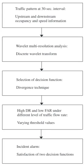
Traffic pattern at 30-sec. interval:

Upstream and downstream

occupancy and speed information

Wavelet multi-resolution analysis:

Discrete wavelet transform

Selection of decision function:

Divergence technique

High DR and low FAR under

different level of traffic flow rate:

Varying threshold values

Incident alarm:

Satisfaction of two decision functions

(3)

of optimal threshold values for incident detection algorithms is an important issue for real-world implementation purposes, there has been little systematic and methodological research in this area. From this perspective, it is advantageous to vary the threshold values based on traffic flow rate. We also derive the mathematical relationship between the false alarm prob-ability and the threshold value of our proposed decision function. As a result, our proposed algorithm, which does vary the threshold values based on traffic condition, yields higher detection rate (DR), lower false alarm rate (FAR) and faster mean

time to detection (MTTD) than other algorithms.Fig. 1illustrates the flowchart of the proposed algorithm for freeway

inci-dent detection. More details on performance comparisons are presented in Section3.

This paper is organized into six sections. A brief review of wavelet and multi-resolution wavelet techniques is given in

Section2. The proposed methodology is presented in Section3, which is followed by the comparison of the employed

algo-rithms in Section4. In Section5, case studies using real-world freeway data are presented. Finally, Section6concludes with a

brief summary as well as suggestions of future research directions.

2. Multi-resolution wavelet technique

2.1. Review of wavelet transform

Wavelet transform, which contains time-scale information, has been recognized as a powerful signal analysis tool (

Vida-kovic, 1999; Jeong et al., 2006a). Wavelets are a family of functions derived from two basis functions,/(t) and

w

(t), known as

the ‘‘father” wavelet and the ‘‘mother” wavelet. Iff(t)

e

L2(R), whereL2(R) is the space of square integrable real functions

de-fined on the real lineR,f(t) is described as the following:

f_ðt_{Þ ¼}X

2L 1

k¼0

cL;k/L;kðtÞ þ

X

J

j¼L

X

2L 1

k¼0

dj;kwj;kðtÞ ð1Þ

where theCL,kanddj,kare the coefficients for the basis function/L,k(t) and

w

j,k(t), respectively.

It is reasonable to assume that traffic measurements collected over time in normal operation, i.e. non-incident, conditions can be expressed as:

y_ðtiÞ ¼fðtiÞ þ

e

ðtiÞ; i¼1;2;. . .;n ð2Þ

wheref(ti) is a true traffic measurement ande(ti) are noises following independent and identically distributed (i.i.d.) normal

distributionN(0,

r

2_{). When a discrete wavelet transform (DWT)}_W_{is used for a}_y_{, it is expressed by}_d₌_Wy_{, where}_d_{is the}

wavelet coefficients andWis the wavelet transform matrix.

The interpretation of relationship between time domain and wavelet domain is important for the detection of the change

point in the wavelet domain. Theorem 1 (Jeong et al., 2006b) below provides a clear understanding of the relationship

be-tween time domain and wavelet domain.

Theorem 1. When there is a mean change of traffic measurements such as flow, speed, or occupancy in

q

iunits of

r

for the time

ti’s in the interval A = (ts, te) with t16ts< ti< te6tn, i.e.,

FnewðtiÞ ¼

F0ðtiÞ þ

q

i

r

; ti2A

F0ðtiÞ; elsewhere

ð3_Þ

wavelet coefficients have the following corresponding shift:

hi;new¼hi;0þdi

r

; i¼1;2;. . .;n ð4Þ

wherehis a wavelet coefficient anddi¼Pj2A

q

hhijand hij’s are the elements of the DWT matrixW(seeJeong et al. (2006b)for the

proof of Theorem 1).

The importance of Theorem 1 is that it warrants that the locations of changes in the time domain can be detected by ana-lyzing the wavelet domain.

2.2. Wavelet multi-resolution analysis on freeway incident detection

The general traffic phenomenon after the occurrence of an incident is the slowing down of vehicular speed and the in-crease in highway occupancy upstream of the incident site. On the other hand, downstream speed will be comparatively

fas-ter and the occupancy lower. Recent incident detection studies (Adeli and Samant, 2000; Samant and Adeli, 2000; Teng and

Qi, 2003) found that wavelet can accurately identify a sharp change in traffic measurements that are obscured by noise. For

example,Adeli and Samant (2000)proposed a wavelet technique to filter out noises and utilized its multi-resolution

prop-erty for incident detection. They selected several wavelet coefficients in different resolution levels by using the filtering method prior to entering the values into neural network models.

(4)

OUD

h i

16¼ fy

ou

t7;y

ou t6;. . .;y

ou

t ;y

od

t7;y

od t6;. . .;y

od

t g

SUD

h i

16¼ fy

su

t7;y

su t6;. . .;y

su

t;y

sd

t7;y

sd t6;. . .;y

sd

t g

whereyou

t ; yodt ; ysut andysdt are upstream and downstream occupancy and speed data at timet. If two-level Haar wavelet

(Teng and Qi, 2003) is adopted, its DWT can be expressed as:

DTWhOUDi¼ co

2;1;c

o

2;2;c

o

2;3;c

o

2;4;d

o

2;1;d

o

2;2;d

o

2;3;d

o

2;4;d

o

1;1;d

o

1;2;d

o

1;3;d

o

1;4;d

o

1;5;d

o

1;6;d

o

1;7;d

o

1;8

h i

16

DTWhSUDi¼ cs

2;1;c

s

2;2;c

s

2;3;c

s

2;4;d

s

2;1;d

s

2;2;d

s

2;3;d

s

2;4;d

s

1;1;d

s

1;2;d

s

1;3;d

s

1;4;d

s

1;5;d

s

1;6;d

s

1;7;d

s

1;8

h i

16

wherecm,nanddm,nare thenth coarser and finer coefficients in scalem, respectively. The equations for these wavelet

coef-ficients are tabulated inTable 1.

Based on the 16 wavelet coefficients, we can develop a new AID algorithm. In Section3, we will discuss how this new

wavelet-based AID algorithm is developed and evaluate the performance using simulated and real-world incident data.

3. Wavelet-based AID algorithm

This section proposes a new AID algorithm, which integrates wavelet multi-resolution analysis with varying threshold values. The significant characteristics of the proposed approach will also be presented.

3.1. Extraction of test statistic for incident detection

Traffic measurements have a tendency to change after the occurrence of an incident. For example, occupancy increases upstream and decreases downstream while the opposite happens to speed. These differences between up- and downstream traffic measurements have been the basis of most freeway AID algorithms such as the California and the Minnesota ones. The California algorithm only utilizes current time occupancy information, which may produce high FAR because of dynamic traffic fluctuations. On the other hand, the Minnesota algorithm employs cumulative sum of differences between up and downstream occupancies in order to alleviate the high FAR setback commonly yielded by the California algorithm.

In the previous section, 16 wavelet coefficients, which contain multi-resolution information, are presented. Finer coeffi-cients present the difference between current and previous measurements, which is similar to the decision functions of Cal-ifornia algorithm, while coarse coefficients illustrate the cumulative sum of traffic measurement for several time windows, which denotes the core component of the decision functions of Minnesota algorithm.

Based onTable 1, we can define the coarser coefficients as follows (in case of occupancy measurement):

Table 1

The equations of each wavelet coefficient.

Occupancy measurement Speed measurement

co

2;1¼ðy ou

t7þyout6Þþðyout5þyout4Þ

ﬃﬃ

4

p cs

2;1¼ðy su

t7þysut6Þþðysut5þysut4Þ

ﬃﬃ

4

p

co

2;2¼ðy ou

t3þyout2Þþðyout1þyoutÞ

ﬃﬃ

4

p cs

2;2¼ðy su

t3þysut2Þþðysut1þysutÞ

ﬃﬃ

4

p

co

2;3¼

ðyod

t7þyodt6Þþðyodt5þyodt4Þ

ﬃﬃ

4

p cs

2;3¼

ðysd

t7þysdt6Þþðysdt5þysdt4Þ

ﬃﬃ

4

p

co

2;4¼ð

yod

t3þyodt2Þþðyodt1þyodtÞ

ﬃﬃ

4

p cs

2;4¼ð

ysd

t3þysdt2Þþðysdt1þysdtÞ

ﬃﬃ

4

p

do2;1¼ð

you

t7þyout6Þþðy

ou

t5þyout4Þ

ﬃﬃ

4

p ds2;1¼ð

ysu

t7þysut6Þþðy

su

t5þysut4Þ

ﬃﬃ

4

p

do2;2¼ð

you

t3þyout2Þþðyout1þyoutÞ

ﬃﬃ

4

p ds2;2¼ð

ysu

t3þysut2Þþðysut1þysutÞ

ﬃﬃ

4

p

do2;3¼ðy od

t7þyodt6Þþðyodt5þyodt4Þ

ﬃﬃ

4

p ds2;3¼ðy

sd

t7þysdt6Þþðysdt5þysdt4Þ

ﬃﬃ

4

p

do

2;4¼ðy od

t3þyodt2Þþðyodt1þyodtÞ

ﬃﬃ

4

p ds

2;4¼ðy sd

t3þysdt2Þþðysdt1þysdtÞ

ﬃﬃ

4

p

do

1;1¼ðy ou

t7yout6Þ

ﬃﬃ

2

p ds

1;1¼ðy su

t7ysut6Þ

ﬃﬃ

2

p

do

1;2¼ðy ou

t5yout4Þ

ﬃﬃ

2

p ds

1;2¼ðy su

t5ysut4Þ

ﬃﬃ

2

p

do

1;3¼ðy ou

t3yout2Þ

ﬃﬃ

2

p ds

1;3¼ðy su

t3ysut2Þ

ﬃﬃ

2

p

do

1;4¼ðy ou

t1youtÞ

ﬃﬃ

2

p ds

1;4¼ðy su

t1ysutÞ

ﬃﬃ

2

p

do1;5¼ðy od

t7yodt6Þ

ﬃﬃ

2

p ds1;5¼ðy

sd

t7ysdt6Þ

ﬃﬃ

2

p

do1;6¼ð

yod

t5yodt4Þ

ﬃﬃ

2

p ds1;6¼ð

ysd

t5ysdt4Þ

ﬃﬃ

2

p

do1;7¼ðy od

t3yodt2Þ

ﬃﬃ

2

p ds1;7¼ðy

sd

t3ysdt2Þ

ﬃﬃ

2

p

do

1;8¼ðy od

t1yodtÞ

ﬃﬃ

2

p ds

1;8¼ðy sd

t1ysdtÞ

ﬃﬃ

2

(5)

co

2;1¼

you

t7þyout6

þ you

t5þyout4

ffiffiffi

4

p ¼ 1ffiffiffi

4

p X

4

j¼1 you

t4jþ1

co

2;2¼

you

t3þyout2

þ you

t1þyout

ffiffiffi

4

p ¼ 1ffiffiffi

4

p X

3

j¼0

you tj

co

2;3¼

yod

t7þyodt6

þ yod

t5þyodt4

ffiffiffi

4

p ¼ 1ffiffiffi

4

p X

4

j¼1

yod

t4jþ1

co

2;4¼

yod

t3þyodt2

þ yod

t1þyodt

ffiffiffi

4

p ¼ 1ffiffiffi

4

p X

3

j¼0

yod tj

Namely,co

2;2co2;4¼p1ﬃﬃ₄ P3

j¼0 youtjyodtj

n o

andco

2;1co2;3¼p1ﬃﬃ₄ P4

j¼1 yout4jþ1yodt4jþ1

n o

.

Therefore, we can obtain several test statistics that are similar to the decision functions of Minnesota algorithm in the wavelet domain as follows:

For occupancy measurements,

WMocc

1 ¼

co

2;2co2;4 max_fco

2;1;co2;3g

¼

1

ﬃﬃ

4 p P3

i¼0 youtiy

od ti

max 1

ﬃﬃ

4 p P4

i¼1yout4iþ1; 1

ﬃﬃ

4 p P4

i¼1yodt4iþ1

n o ð5Þ

WMocc2 ¼ co

2;2co2;4

co

2;1co2;3

max_fco

2;1;co2;3g

¼ 1

ﬃﬃ

4

p P3

i¼0 youtiyodti

P4

i¼1 yout4iþ1yodt4iþ1

max 1

ﬃﬃ

4 p P4

i¼1yout4iþ1;p1ﬃﬃ₄

P4

i¼1yodt4iþ1

n o ð6Þ

For speed measurements,

WMspe

1 ¼

cs

2;2cs2;4 maxfcs

2;1;cs2;3g

¼

1

ﬃﬃ

4 p P3

i¼0ðy

su tiysdtiÞ

max 1

ﬃﬃ

4 p P4

i¼1ysut4iþ1; 1

ﬃﬃ

4 p P4

i¼1ysdt4iþ1

n o ð7Þ

WMspe

2 ¼

ðcs

2;2cs2;4Þ ðc

s

2;1cs2;3Þ

maxfcs

2;1;cs2;3g

¼ 1

ﬃﬃ

4

p P3

i¼0ðy

su

tiy

sd

tiÞ

P4

i¼1ðy

su

t4iþ1ysdt4iþ1Þ

max 1

ﬃﬃ

4 p P4

i¼1ysut4iþ1; 1

ﬃﬃ

4 p P4

i¼1ysdt4iþ1

n o ð8Þ

It is worth noting that the relationship between Minnesota algorithm and wavelet-based test statistic can be extracted by

comparing Eqs.(5) and (6). The Minnesota algorithm (Stephanedes and Chassiakos, 1993) may be expressed as

M1_¼ 1

n

Pn1

i¼0youti

Pn1

i¼0yodti

max 1

m

Pm

i¼1youtniþ1; 1

m

Pm

i¼1yodtniþ1

ð9Þ

M2_¼ 1

n

Pn1

i¼0youti

Pn1

i¼0yodti

1

m

Pm

i¼1youtniþ1

Pm

i¼1yodtniþ1

max 1

m

Pm

i¼1youtniþ1; 1

m

Pm

i¼1yodtniþ1

ð10Þ

When n is equivalent to m and both are 4, Eqs. (5) and (6) are the same as the Minnesota algorithm, representing

WMocc1 ¼M1 andWM

occ

2 ¼M2. Thus, the Minnesota algorithm is a special case of our proposed algorithm. By applying the

wavelet multi-resolution analysis to traffic information, meaningful test statistic can be extracted for incident detection. The next task is to select the best test statistic and develop a systematic method of varying threshold values depending on the level of traffic volume.

3.2. Selection of best test statistic for incident detection

In the previous section, several test statistics (Eqs.(5)–(8)and finer coefficients) were extracted for incident detection by

using wavelet multi-resolution analysis. Given these test statistics, the major task is to select the one that is most capable of clearly discriminating between normal and incident-disturbed traffic conditions. Divergence, which can be used as a class

separability measure with respect to the adopted feature, is popular among other feature selection techniques (Guyon

and Elisseeff,2003; Theodoridis and Koutroumbas, 2006). Assuming that the density functions of feature vectorxifor

inci-dent data andxjfor incident-free data are GaussiansN(

l

i,Ri) andN(

l

j,Rj), respectively, we can compute the divergenceJij(x)

as:

JijðxÞ ¼ 1 2trace R

1

I RjþR1j Ri2I

n o

þ1₂ðliljÞ T

ðR1_i _þR1_j _Þlilj

ð11_Þ

where

l

i,Ri,

l

jandRjare means and covariances ofxiandxj, andIis identity matrix.

(6)

JijðxÞ ¼ 1 2

r

2

j

r

2

i

þ

r

2

i

r

2

j

2

!

þ1₂ðliljÞ

2 1

r

2

i

þ

_r

12

j

!

ð12Þ

where

l

i,

l

jand

r

2i,

r

2j are the means and variances ofxiandxj, respectively.

In order to determine the best test statistic using divergence technique, seven simulation scenarios covering different

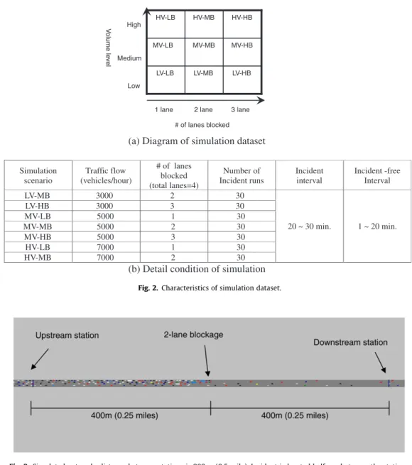
lev-els of traffic demand and incident severity conditions were implemented using VISSIM micro-simulation software (PTV

Vi-sion, 2007). The scenarios were divided according to traffic demand (low, medium, and high volume, labeled as LV, MV, and HV respectively) and incident severity (low, medium, and high blockage, labeled as LB, MB, and HB). The characteristics of

the simulation scenarios are summarized inFig. 2. As shown inFig. 2, the blockage level is determined by the number of

lanes blocked; that is, LB, MB, and HB relates to one, two, or three lanes blocked, respectively. The blockage was performed by making vehicles stop for 10 min at traffic a signal located halfway between the detector stations, which were 0.5 miles (800 m) apart from each other. The simulated roadway facility consisted of a four-lane freeway. The traffic-demand levels LV,

MV, and HV correspond to flow rates of 3000, 5000, and 7000 veh/h/4lanes.Fig. 3shows a snapshot of a simulation-run

un-der scenario HV–MB. Among the nine possible scenarios tabulated, two were excluded from the analysis: LV–LB and HV–HB. The LV–LB, or low-demand and low-blockage condition is excluded because it has minimum adverse effect on the traffic and is very challenging to detect. On the other end of the spectrum, the HV–HB, or high-demand and high-blockage condition is also excluded because while it does have significant impact on traffic, it is very easy, if not trivial, to detect with a wide range of methods.

(a) Diagram of simulation dataset

Simulation scenario

Traffic flow (vehicles/hour)

# of lanes blocked (total lanes=4)

Number of Incident runs

Incident interval

Incident -free Interval

LV-MB 3000 2 30

LV-HB 3000 3 30

MV-LB 5000 1 30

MV-MB 5000 2 30

MV-HB 5000 3 30

HV-LB 7000 1 30

HV-MB 7000 2 30

20 ~ 30 min. 1 ~ 20 min.

(b) Detail condition of simulation

LV-HB LV-MB

LV-LB

MV-HB MV-MB

MV-LB

HV-HB HV-MB

HV-LB

# of lanes blocked

V

o

lume le

ve

l

1 lane 2 lane 3 lane Low

Medium High

Fig. 2.Characteristics of simulation dataset.

(7)

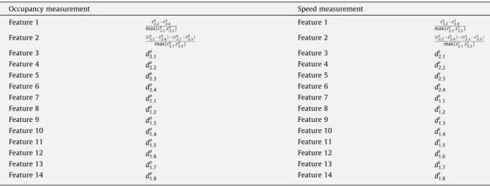
Table 2shows the several test statistics of occupancy and speed measurements that include the test statistics of California and Minnesota algorithms. We chose occupancy and speed for the proposed algorithm because algorithms based on them

were found to be more efficient than those based only on one traffic parameter (Mak and Fan, 2005). It has been reported

that speed and occupancy data tend to reflect incident-induced lane-blockage in a timelier manner than flow data (Mak and

Fan, 2005).

Based on the divergence results summarized inTable 3, Feature 1 yields the highest divergence values and, hence, is the

best test statistic for both occupancy and speed measurements (seeFig. 4). Feature 1 provides an indication of the traffic

conditions in the freeway segment that lies between the two detectors because Feature 1 represents the cumulative spatial difference between upstream and downstream traffic measurements (occupancy and speed). Therefore, higher Feature 1 can be attributed to congestion created between the two detectors as a result of an incident or a bottleneck. Note that the effect of incidents on traffic is more temporary and sharper frequency on traffic measurements than that of bottleneck. For the cases of LV–MB and MV–LB, it is less clear which among the 16 is the best feature because they are not noticeably discrim-inating between normal and incident-disturbed traffic cases. However, Feature 1 presents the best performance, in general, among all candidate features.

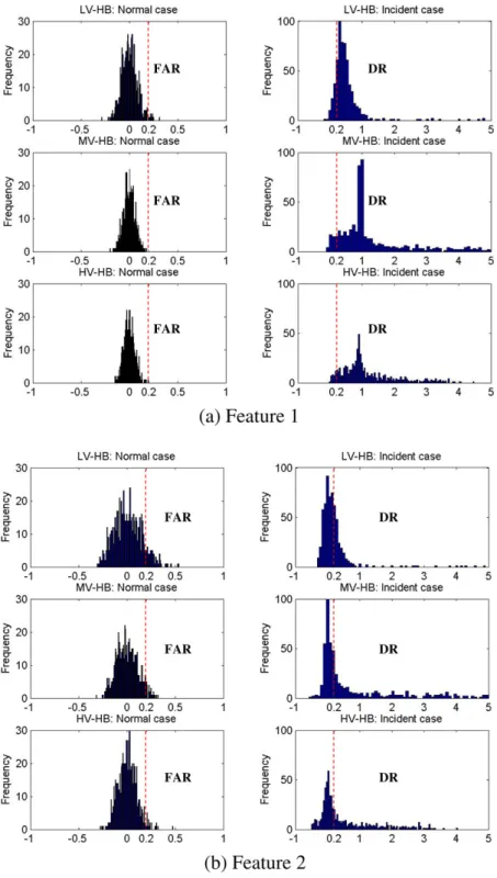
Fig. 4consists of a battery of histograms based on various scenarios for the comparison of the two best and the worst

occupancy-based features: Features 1, 2 and 6.Fig. 4empirically shows that good features should have lower FAR under

nor-mal traffic conditions while larger DR under incident casesregardless of the level of traffic flow. The histograms on the left-side

relate to the incident-free condition whereas the ones on the right-side represent incident cases. When the observed test

Table 2

Several test statistics for incident detection.

Occupancy measurement Speed measurement

Feature 1 co

2;2co2;4 maxfco

2;1;co 2;2g

Feature 1 cs

2;2cs2;4 maxfcs

2;1;cs 2;2g

Feature 2 ðco

2;2co2;4Þðco2;1co2;3Þ maxfco

2;1;co 2;2g

Feature 2 ðcs

2;2cs2;4Þðcs2;1cs2;3Þ maxfcs

2;1;cs 2;2g

Feature 3 do

2;1 Feature 3 ds2;1

Feature 4 do2;2 Feature 4 d

s

2;2

Feature 5 do

2;3 Feature 5 ds2;3

Feature 6 do

2;4 Feature 6 ds2;4

s

1;1

Feature 8 do1;2 Feature 8 ds1;2

Feature 9 do

1;3 Feature 9 ds1;3

s

1;4

Feature 11 do1;5 Feature 11 ds1;5

Feature 12 do

1;6 Feature 12 ds1;6

s

1;7

s

1;8

Table 3

Divergence of candidate features.

F1 F2 F3 F4 F5 F6 F7 F8 F9 F10 F11 F12 F13 F14

(a)Occupancy measurement

LV–MB 0.1 0.0 0.0 0.0 0.0 0.0 0.0 0.0 0.0 0.0 0.0 0.1 0.2 0.3

LV–HB 58.8 10.6 0.1 19.6 0.0 0.2 0.0 0.1 2.1 5.2 0.1 0.3 0.7 1.5

MV–LB 0.1 0.0 0.0 0.0 0.0 0.0 0.0 0.0 0.0 0.0 0.0 0.0 0.1 0.1

MV–MB 134.4 24.3 5.5 19.2 0.1 0.3 0.2 1.5 3.5 5.5 0.2 0.3 0.5 0.7

MV–HB 786.5 150.9 69.0 67.1 0.1 0.2 14.6 15.4 16.0 15.9 0.2 0.3 0.5 0.7

HV–LB 36.2 6.3 1.8 3.2 0.1 0.2 0.3 0.6 0.9 1.2 0.1 0.2 0.5 0.5

HV–MB 350.7 57.5 29.6 33.5 0.1 0.2 7.8 8.4 9.7 10.8 0.2 0.4 0.9 1.1

Average 195.3 35.7 15.1 20.4 0.1 0.2 3.3 3.7 4.6 5.5 0.1 0.2 0.5 0.7

(b)Speed measurement

LV–MB 13.8 0.1 0.1 0.0 8.8 11.6 0.1 0.0 0.1 0.1 7.4 9.7 11.1 9.7

LV–HB 436.1 57.2 4.6 12.5 6.7 7.2 0.6 1.3 2.2 2.1 6.4 7.7 8.4 6.6

MV–LB 5.2 0.0 0.0 0.0 0.0 0.0 0.0 0.0 0.0 0.0 0.0 0.0 0.0 0.0

MV–MB 1269.1 183.5 21.3 38.7 0.3 0.2 2.6 4.0 6.5 8.5 0.2 0.2 0.3 0.3

MV–HB 6504.1 567.7 105.5 98.9 4.4 5.1 16.4 16.0 16.1 16.4 4.5 5.3 5.9 6.3

HV–LB 735.5 119.7 22.7 35.2 0.0 0.1 4.4 7.1 9.4 11.8 0.0 0.0 0.0 0.1

HV–MB 6191.3 544.1 115.6 118.4 0.1 0.2 31.8 34.2 36.5 38.1 0.1 0.1 0.1 0.1

(8)

statistic value is greater than the threshold value (dotted vertical line), an ‘‘incident alarm” is sounded. The ideal feature/ threshold combination would place all incident-free observations to the left of the threshold line and all incident cases to

the right of it, thus yielding a 100% DR and 0% FAR. As shown inFig. 4, when the threshold value is set to 0.2, Feature 1

(Fig. 4a) detects almost all incident cases while keeping its FAR low in comparison to those of Feature 2 (Fig. 4b). Therefore, Feature 1 attains higher DR and low FAR compared to those of Feature 2. On the other hand, as suggested by the divergence

results, Feature 6 (Fig. 4c) shows little discrimination between normal and incident cases. Results from speed measurements

present a similar phenomenon. In addition, depending on the level of traffic flow in normal traffic conditions, variance

(9)

changes slightly even if the mean is almost zero for all cases. As such fixed, or pre-determined, threshold values tend to yield

higher FAR values. More details onvaryingthreshold values are presented in Section3.3.

Based on these results, Feature 1 will be used as the decision functions, for both occupancy and speed measurements, as

shown in Eqs.(5) and (7).

3.3. Varying threshold values

In Section3.2, two test statistics based on divergence criterion were selected for incident detection. It has been observed

repeatedly that shortly after the occurrence of an incident, occupancy tends to increase upstream and decrease downstream while the opposite happens to speed. Therefore, two decision functions for incident detection are proposed as the following:

WMocc1 ¼

1

ﬃﬃ

4 p P3

i¼0ðyoutiyodtiÞ

max 1

ﬃﬃ

4 p P4

i¼1yout4iþ1; 1

ﬃﬃ

4 p P4

i¼1yodt4iþ1

n o>docc ð13Þ

WMspc1 ¼

1

ﬃﬃ

4 p P3

i¼0ðysutiysdtiÞ

max 1

ﬃﬃ

4 p P4

i¼1ysut4iþ1;p1ﬃﬃ₄

P4

i¼1ysdt4iþ1

n o<dspe ð14Þ

In other words, an incident alarm is sounded only when the conditions in both Eqs.(13) and (14)are met. The most

impor-tant issue is how to select optimal threshold valuesdoccanddspe. Even though there was a research (ITS DECISIONS, 2001) to

try to find out an optimal threshold values, little published study has reported a theoretical approach to the optimal selection of such parameters. In order to derive the mathematical relationship between the false alarm probability and the threshold values of proposed decision functions, firstly, we can mathematically express false alarm rate as follows:

a

t¼PðWMocc1 >docc;WMspe₁ <dspejnormal trafficÞ ð15Þ

whereWMocc1 andWM

spe

1 are normal distributionsNð

l

0;occ;

r

20;occÞandNð

l

0;spe;

r

20;speÞ, respectively, and

a

tis the target or

desir-able false alarm rate. Under incident-free traffic conditions, usually

l

0,occ= 0 and

l

0,spe= 0. Assuming thatWMocc1 andWM

spe

1

are independent, we obtain:

a

t¼P WMocc1 >doccjnormal traffic

P WMspe

1 <dspejnormal traffic

¼ 1

U

docc

l

0;occ

r0

;occ

U

dspe

l

0;spe

r0

;spe

ð16Þ

(10)

whereUdenotes the cumulative distribution function of a standard normal distribution. By assuming that each term

con-tributes equally to

a

tin Eq.(16), we can obtain the following approximated equations:

ffiffiffiffiffi

a

t

p

1

U

doccl0;occ

r0;occ

ffiffiffiffiffi

a

t

p

_U

dspel0;spe

r0;spe

ð17Þ

Because

l

0;occ¼0 and

l

0;spe¼0 under incident-free traffic conditions, the relationship between the false alarm probability

and the threshold values can be found using the following equations:

docc¼

U

1_ð1p_affiffiffiffi_t_Þ

r0

;occ dspe¼

U

p1ffiffiffiffiat

r0

;spe

ð18_Þ

(11)

whereU1_{represents the inverse of the cumulative distribution function of a standard normal distribution. As we can see in}

Eq.(18), for a given target false alarm rate (

a

t), the threshold values will be changed adaptively depending on the traffic

lev-els of normal traffic, i.e., the standard deviations_ð

r

0;occ;

r

0;speÞofWMocc1 andWM

spe

1 under normal traffic conditions.

With all the building blocks in place,Fig. 5illustrates the core procedure of the proposed incident algorithm.

4. Case study with simulated data

To evaluate the proposed wavelet-based AID algorithm, its performance is compared with that of California, Minnesota,

and several neural network models. In this section, seven simulated incident scenarios, as presented previously in Section3.1

andFig. 2, are used for that purpose. Further comparisons using real-world incident cases are presented in Section5. To obtain the optimal values of the varying threshold parameters, which change with the level of traffic volume, both the

means and the variances of the test statisticsWMocc1 andWM

spe

1 under normal traffic must be known beforehand. This is

accomplished by computingWMocc

1 andWM

spe

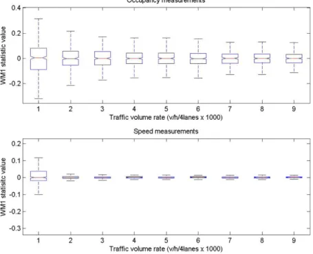
1 for different levels of normal traffic conditions.Fig. 6shows the box plots

of test statistics for different traffic levels from very light traffic, about 250 veh/h/lane, to the left, to near-capacity traffic,

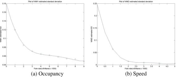
over 2000 veh/h/lane to the right. It is interesting to note inFigs. 6 and 7, that whereas the means of test statistics are

(12)

tically zero across all traffic levels, their standard deviation decreases as the traffic volume increases. This is evidence that

any type of comparative AID algorithm that is based on threshold parameters such asWMocc

1 andWM

spe

1 needs to vary the

parameters based on the traffic level in order to minimize false alarms and maximize detection rates.

Based on the experimental results, we can approximate the standard deviation curve over traffic flow rate with fourth-degree polynomial functions as the following:

^

r0

;occ¼0:0001x4vol0:0022x

3

volþ0:0195x

2

vol0:0777xvolþ0:1798 ð19Þ

^

r

spe¼

0:0018x4_vol0:0251x3_volþ0:1282x2_vol0:2859xvolþ0:245 forxvol5

0:005 forxvol>5

(

ð20Þ

where

r

^occand

r

^speare the estimated standard deviations ofWMocc1 andWM

spe

1 in normal traffic, andxvolis the four-lane

traf-fic flow rate per hour divided by 1000.Fig. 8shows the estimated curve of standard deviation over different traffic flow rates.

InFig. 8, the small circle represents the actual standard deviation value at specific traffic volume rate. The estimated curve can fit the standard deviation very well.

In order to evaluate the incident detection performance of the proposed algorithm, a total of 210 simulation ‘‘runs” or cases, 30 for each of the 7 scenarios, were generated with different random-seeds. In each scenario, the runs were performed

using themulti-runfeature of VISSIM, with the first run having seed equals to 1, and the last run having

random-seed equal to 30. The length period of each run was 60 min, with the incident (blockage) from starting att= 20 min and

end-ing att= 30 min. The 30 cases of each scenario were then randomly divided into two groups – 15 for training and the other

15 for testing purposes. As a result, a total of 105 (157) incident cases were available for training and the same amount

was available for testing. As for the incident-free cases, a run of 4 h was performed for each traffic demand level.

As commonly adopted in AID studies, the measures of effectiveness (MOE) used were the detection rate (DR), false alarm rate (FAR), and mean time to detection (MTTD). DR is calculated as the ratio of the number of detected incidents to the total number of incidents in the data set. FAR is defined as the ratio of the number of false alarms to the total number of appli-cations of the algorithm, generally every 30 s, under incident-free conditions. MTTD is simply the average time from the occurrence of an actual incident till the correct detection of the incident for all detected incidents. Obviously, it is desirable for AID algorithms to yield high DR (near 100%), low FAR (near 0%), and short MTTD (as short as possible).

In an effort to evaluate the proposed wavelet-based AID algorithm, four algorithms were selected for comparison. These

include: California algorithm, Minnesota algorithm, wavelet-based radial basis function (WRBF) neural networks (Karim and

Adeli, 2002), wavelet-based multi-layer feed-forward neural networks (WMLF1 and WMLF2), and multi-layer feed-forward neural networks (MLF1 and MLF2). California algorithm and Minnesota algorithm are well-established and widely-tested.

WMLF1, which relies on occupancy data alone, and WMLF2, which employees both occupancy and speed data, use wave-let coefficients as neurons in the input layers of the neural network. This algorithm is based on the wavewave-let-filtering scheme

proposed byGhosh-Dastidar and Adeli (2003). The architecture of WMLF algorithms consists of 6 neurons in the input layer

for WMLF1 and 12 neurons for WMLF2, a single hidden layer with 10 neurons, and one output neuron. Tangent sigmoid function and linear transfer function are used for activation function in the hidden and output layers. WRBF, which employs occupancy, speed, and flow data, also use wavelet coefficients as neurons in the input layers of RBF neural network.

The architecture of MLF algorithms is identical to WMFL algorithms, except for the input neurons. MLF1 uses occupancy

data only as eight input neurons (upstream and downstream occupancy: (t3), (t2), (t1) and (t)), while MLF2

com-bines both occupancy and speed data as 16 input neurons (upstream and downstream occupancy and speed: (t3),

(t2), (t1) and (t)). In other words, MLF employs raw traffic data as input neurons instead of wavelet coefficients.

(13)

Table 4

Performance comparison (simulation dataset).

dCal1 dCal2 d3Cal California algorithm dMinn1 dMinn2 Minnesota algorithm

DR (%) FAR (%) MTTD (s) DR (%) FAR (%) MTTD (s)

(a)Training dataset

1 0.45 0.07 70 1 307 0.15 0.17 85 1 209

1 0.39 0.05 75 3 247 0.04 0.21 90 3 191

1 0.35 0.05 81 5 228 0.09 0.01 98 5 121

1 0.31 0.09 88 7 216 0.08 0.01 100 7 114

a

Th. WRBF Th. WMFL1 Th. WMFL2

DR (%) FAR (%) MTTD (s) DR (%) FAR (%) MTTD (s) DR (%) FAR (%) MTTD (s)

0.9 90 1 160 0.9 85 1 201 0.9 95 1 165

0.8 98 2 150 0.8 98 2 160 0.8 98 2 152

0.7 99 3 144 0.7 99 3 144 0.7 100 3 144

0.6 100 4 136 0.6 100 4 131 0.6 100 4 137

Th. MFL1 Th. MFL2 at Proposed algorithm

DR (%) FAR (%) MTTD (s) DR (%) FAR (%) MTTD (s) DR (%) FAR (%) MTTD (s)

0.9 88 1 170 0.9 96 1 246 0.01 99 0.7 169

0.8 97 2 162 0.8 99 2 207 0.03 100 0.8 160

0.7 99 3 148 0.5 100 4 191 0.05 100 0.8 156

0.6 100 4 147 0.4 100 6 175 0.07 100 0.8 147

Algorithm Threshold value DR (%) FAR (%) MTTD (s)

(b)Testing dataset

Proposed algorithm docc¼Uð11pffiffiffi_a

tÞr0;occ

rspeUp1ffiffiffiffiatr0;spe

99 1 150

California algorithm dCal

1 ¼1;dCal2 ¼0:45;dCal3 ¼0;07 73 2 270

Minnesota algorithm dMinn1 ¼0:15;dMinn2 ¼0:17 80 1 223

WRBF Th. = 0.9 93 1 155

WMFL1 Th. = 0.9 92 1 161

WMFL2 Th. = 0.9 95 1 158

MFL1 Th. = 0.9 88 1 170

MFL2 Th. = 0.9 92 1 242

a

Th.: Threshold value.

Table 5

Detailed performance of the proposed algorithm.

at LV

docc dspe MB HB

0.01 U1

ð1pffiffiffi_a

tÞr0;occ U

1

ffiffiffiffi

at

p r0;spe 93 2 234 100 2 164

0.03 100 2 246 100 2 164

0.05 100 2 234 100 2 154

0.07 100 2 220 100 2 154

at MV

docc dspe LB MB HB

DR (%) FAR (%) MTTD (s) DR (%) FAR (%) MTTD (s) DR (%) FAR (%) MTTD (s) 0.01 U1

ð1pffiffiffi_a

tÞr0;occ U

1

ffiffiffiffi

at

p r0;spe 100 0 268 100 0 128 100 0 108

0.03 100 0 236 100 0 128 100 1 108

0.05 100 1 226 100 0 128 100 1 108

0.07 100 1 190 100 0 120 100 1 108

at HV Average

docc dspe LB MB

DR (%) FAR (%) MTTD (s) DR (%) FAR (%) MTTD (s) DR (%) FAR (%) MTTD (s) 0.01 U1

ð1pffiffiffi_a

tÞr0;occ U1ffiffiffiffi_a

t

p r0;spe 100 0 108 100 0 176 99 0.7 169

0.03 100 0 158 100 0 84 100 0.8 160

0.05 100 0 156 100 0 84 100 0.8 156

(14)

Table 4presents the results of performance comparison of different incident detection algorithms for training and testing

data sets. InTable 4,dCal₁ ,dCal₂ , anddCal₃ represent the threshold values in California algorithm anddMinn₁ ;dMinn₂ present the

threshold values in Minnesota algorithm. In addition, varying threshold values in the proposed algorithm were described bydoccanddspe.Table 4shows the best performance each algorithm can achieve for a given level of FAR. For the purpose

of fair comparisons, we fixed the threshold values to those that yielded the best performance for the training dataset and

these threshold values were used to obtain the performance for testing data set. InTable 4, we emphasize the comparison

parts with bold fonts.

In this experiment, threshold values were selected to achieve a FAR of 1% for training performance. As shown inTable 4b,

the proposed AID algorithm clearly outperformed others with a 99% DR, 1% FAR, and 150 s. MTTD for the testing data set. Within the WMLF family, WRBF showed good performance compared to other neutral networks, especially faster MTTD than other algorithms. In addition, WMLF2 yielded a higher DR than WMLF1, arguably because WMLF2 employed more traffic information than WMLF1 did.

To further explore the effectiveness of the proposed algorithm, its performance under each simulated scenario is

tabu-lated inTable 5. It is evident, and not surprisingly, that higher traffic volume results in high DRs and low FARs irrespective

of the number of lanes blocked because any incident that occurs during high traffic volume causes obvious incident pattern in the denoised traffic data. In this Table, we highlight the best average performance with 1% FAR.

Overall, the proposed wavelet-based AID algorithm consistently yielded the best DR, lowest FAR, and shortest MTTD. In addition, of the four remaining algorithms, the WRBF algorithms yielded higher DR and fast MTTB than those from other neutral network algorithms. This is indicative of the effectiveness of wavelet-based algorithms in filtering out traffic data noises for incident detection purposes. At this point, the proposed algorithm seems very promising and is ready to be tested with real-world incident cases.

5. Case study with real-world data: development of a new incident database

5.1. Real-world dataset description

One of the major challenges of AID research has been the scarcity of incident field data. Therefore, even some very recent

studies have been based solely on simulations (Crabtree and Stamatiadis, 2007; Cheu et al., 2002). The main reason for this is

the difficulty in obtaining accurate incident information that is precise and complete enough for AID research purposes; ba-sic information such as incident start time and location are often not precisely, and occasionally erroneously, reported on incident record systems such as those maintained by freeway patrols and incident management programs. The inaccuracy and imprecision of such reports is often inherent to the data collection process; for instance, the recorded start time of an incident usually comes from the perception of those involved in the incident, or merely from a rough estimate or guess from the officer filing the crash report. Even in the fortuitous case of someone actually observing a crash scene as it unfolded be-fore him, the time he read from his watch and later reported very likely may not be in sync with the real-time traffic data being collected at a traffic management center (TMC) elsewhere. This difference between the unsynchronized watch of a for-tuitous witness and the computer clock at TMC, may it be a couple of minutes or even more, would embed an undesirable time shift in the incident data.

This problem has kept researchers from computing, and, hence, optimizing the MTTD of their respective AID algorithms

correctly (Teng et al., 1999). Besides, it is known that a portion of incidents is never reported, according toRoess et al. (2004).

It is estimated that approximately only 50% of all traffic incidents are recorded on any type of incident log. This casts a sha-dow on some so-called normal traffic data as they might not be really incident-free and are, therefore, unsuitable for algo-rithm training purposes.

In light of these data quality challenges and the importance of evaluating and validating AID algorithms, some efforts have been made towards the creation of incident data sets that are accurate enough for research purposes. These include

Browne et al. (2005), Mak and Fan (2006b), andRoy and Abdulhai (2003). For instance, a relatively well-known database containing information of traffic and incident on a section of interstate I-880 was developed to investigate the effectiveness

of the Freeway Patrol Service (FPS) program in California (Petty et al., 1996; Skabardonis et al., 1997). A similar incident data

collection work was performed on freeway I-10 in Los Angeles area (Skabardonis et al., 1999). Since its creation, the I-880

incident database has been used in several studies including those ofJin et al. (2002), Yuan and Cheu (2003), andSrinivasan

et al. (2005).

As a part of the effort presented in this paper, we decided to create and use a new incident dataset, instead of using any

existing incident database, for two main reasons. First, the Freeway Performance Measurement System (PeMS) (http://

www.pems.eecs.berkeley.edu) has made their 30-s loop detector data available to the public. The richness of spatio– temporal traffic information provided by PeMS, along with the incident record of the California Highway Patrol, also available though PeMS, has made it possible to construct a database that contains accurate incident information for the pur-poses of this study. Second, the new incident dataset resultant from our research adds to the resource of the field of AID study.

For this study, the northbound facility of Interstate 880, or I-880N, was selected as the ‘‘test bed” because this section of freeway was studied before and was deemed to have one of the highest crash frequencies in the San Francisco Bay Area,

(15)

dataset on the same interstate could foster comparative studies related to safety, e.g. incident frequency, by comparing safety information from the database developed in the past and the one developed herein. For this research, 30-s and 5-min lane-by-lane loop detector data were collected for all of the 79 vehicle detector stations (VDS) along I-880N from Sep/01/2006 to Nov/15/2006.

The researchers studied the California Highway Patrol (CHP) incident log and scrutinized the corresponding PeMS traffic data for the VDS pair just upstream and downstream of each incident site. The start time of an incident was defined to be one

interval before the traffic disturbance started, an approach similar to those implemented byMak and Fan (2006a). This was

done by a thorough visual inspection of the 30-s time series of flow and occupancy data for both up and downstream VDS sites.

5.2. Evaluation results

A total of 40 real-world incident data sets were collected along I-880N for the training and testing of the AID algorithms.

In order to provide an idea of the severity of the collected incidents,Fig. 9shows the histogram of the number o lanes

blocked according to the CHP reports. It is important to note that number of lanes blocked equal to zero means that the

0 1 2 3 4

0 2 4 6 8 10 12 14

Number of lanes blocked

N

u

m

b

er

of

i

n

ci

dent

s

Lane Blockage - CHP reports

Fig. 9.Histogram of reported number of lanes blocked by the incident. I-880 is for the most part a 4-lane freeway.

0 5 10 15 20 25 30 35 40

0 20 40 60 80 100 120 140 160 180 200

Incident #

D

u

ra

ti

o

n

(mi

n

u

te

s

)

Incident Duration - CHP reports

(16)

Table 6

Training and testing performance of real-life dataset.

(a) Training dataset subset dCal1 dCal2 d3Cal California algorithm dMinn1 dMinn2 Minnesota algorithm *

1 1 0.83 0.05 50 0 166 0.33 0.85 77 0 98

1 0.65 0.05 87 1 130 0.38 0.59 90 1 92

1 0.59 0.05 93 2 120 0.25 0.49 97 2 88

2 1 0.61 0.31 63 0 153 0.22 0.82 73 0 95

1 0.43 0.21 90 1 123 0.22 0.57 90 1 93

1 0.43 0.15 97 2 120 0.22 0.34 97 2 90

3 1 0.83 0.05 53 0 113 0.33 0.85 67 0 86

1 0.63 0.17 87 1 125 0.31 0.56 87 1 92

1 0.55 0.15 93 2 119 0.41 0.40 97 2 94

4 1 0.83 0.05 60 0 188 0.33 0.85 73 0 102

1 0.69 0.21 83 1 154 0.22 0.56 90 1 102

1 0.59 0.11 93 2 119 0.22 0.41 97 2 95

Subset Th. MFL1 Th. MFL2

1 0.09 63 1 241 0.09 50 1 196

0.08 90 2 236 0.08 80 2 207

0.07 97 3 203 0.07 97 3 196

2 0.09 57 1 213 0.09 73 1 268

0.08 93 2 208 0.08 93 2 240

0.07 97 3 181 0.07 97 3 174

3 0.09 57 1 254 0.09 70 1 224

0.08 67 2 204 0.08 83 2 212

0.07 93 3 184 0.07 93 3 194

4 0.09 87 1 236 0.09 73 1 268

0.08 93 2 210 0.08 90 2 222

0.07 97 3 182 0.07 93 3 156

Subset Th. WMFL1 Th. WMFL2

1 0.09 63 1 297 0.09 67 1 261

0.08 93 2 161 0.08 93 2 111

0.07 97 3 143 0.07 97 3 106

2 0.09 90 1 178 0.09 77 1 150

0.08 93 2 145 0.08 93 2 113

0.07 97 3 137 0.07 97 3 96

3 0.09 67 1 188 0.09 70 1 211

0.08 87 2 173 0.08 93 2 174

0.07 93 3 155 0.07 97 3 125

4 0.09 77 1 193 0.09 83 1 188

0.08 90 2 157 0.08 93 2 152

0.07 97 3 138 0.07 97 3 137

Subset Th. WRBF at docc dspe Proposed algorithm

1 0.09 70 1 137 0.01 U1

1pffiffiffi_a

tr0;occ U

1 1pffiffiffi_a

tr0;spe

97 1 73

0.08 93 2 98 0.03 97 2 66

2 0.09 87 1 91 0.01 97 0 88

0.08 93 2 87 0.03 100 1 80

3 0.09 70 1 110 0.01 93 1 77

0.08 93 2 107 0.03 97 2 65

4 0.09 87 1 109 0.01 97 1 88

0.08 93 2 98 0.03 97 2 76

(b) Testing dataset subset dCal1 dCal2 dCal3 California algorithm

DR (%) FAR (%) MTTD (s)

1 1 0.65 0.05 90 1 165

2 1 0.43 0.21 90 8 113

3 1 0.63 0.17 90 0 193

4 1 0.69 0.21 50 0 132

(17)

report only mentions that the vehicles involved were on the right shoulder or on the center divider. Therefore, the incident

might have blocked the traffic before the arrival of the CHP officers.Fig. 10provides a plot of the reported duration of the

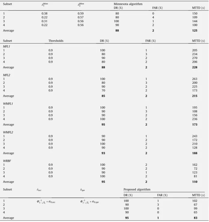
incidents. The missing points on that plot mean that no information regarding the incident duration was reported. Because of the limited number of incident cases, a fourfold cross-validation (CV) procedure was implemented for the comparison of testing performance of different algorithms. In other words, a total of 40 incident cases were divided into four subsets where each subset consists of 10 incident cases. For each experiment, three of the subsets were used for training and the remaining one was used for testing. All incident cases in the dataset were eventually used for both training and testing purposes.

Table 6tabulates the training and testing performance of five AID algorithms for average and for each fold of the fourfold CV. For easy comparisons, we highlight the average performances of each algorithm with bold fonts. Once again, it is evident that the proposed algorithm, showing high DR, low FAR, and fast MTTD, outperformed all the others. For instance, the

pro-Subset dMinn1 dMinn2 Minnesota algorithm

1 0.38 0.59 80 0 150

2 0.22 0.57 80 4 109

3 0.31 0.56 100 1 144

4 0.22 0.56 90 2 100

Average 88 2 125

Subset Thresholds DR (%) FAR (%) MTTD (s)

MFL1

1 0.9 100 1 205

2 0.9 80 3 234

3 0.9 90 2 270

4 0.9 80 2 206

Average 88 2 228

MFL2

1 0.9 100 1 263

2 0.9 80 3 200

3 0.9 90 2 225

4 0.9 70 2 173

Average 85 2 215

WMFL1

1 0.9 100 1 195

2 0.9 90 3 108

3 0.9 90 2 156

4 0.9 100 2 236

Average 95 2 173

WMFL2

1 0.9 90 1 243

2 0.9 90 2 172

3 0.9 100 2 210

4 0.9 90 2 128

Average 93 2 188

WRBF

1 0.9 100 2 162

2 0.9 90 2 72

3 0.9 90 1 123

4 0.9 100 2 81

Average 95 2 110

Subset docc dspe Proposed algorithm

1 U1

1pffiffiffi_a

tr0;occ U11pffiffiffi_a

tr0;spe 100 1 102

2 90 3 67

3 100 0 99

4 90 0 65

Average 95 1 83

(18)

posed algorithm presents on an average 95% DR, 1% FAR, and 83 s. MTTD, which is the best performance among the five AID algorithms. Particularly noteworthy is in the MTTD department where the proposed algorithm is the fastest to correctly de-tect the incidents. Similar to the results when simulated incident scenarios were used, WREF algorithm yielded higher DR and faster MTTD than other neural networks family. Also, WMFL algorithms showed good performance in comparison to those of MFL algorithms.

Overall, the proposed algorithm yielded high DR, low FAR, and fast MTTD in comparison with other well established or neural-net based algorithms for both simulated and real-world scenarios. It is clear that the proposed algorithm is a superior alternative for freeway incident detection applications.

6. Conclusions

This paper proposed a novel wavelet-based freeway automated incident detection algorithm, which utilizes both occu-pancy and speed data. In addition, this research recognized the importance of developed varying threshold values as a func-tion of traffic flow rate. The algorithm was implemented and tested with simulated and real-world incident data sets, which were newly created via VISSIM simulation and data collection on I-880N.

Results of the comparative evaluation effort indicates that overall, wavelet-based algorithm with adaptive thresholding parameters yielded better performance, in most of cases, with higher DR, lower FAR, and faster MTTD. Particularly, since the threshold values can be adaptively changed depending on the traffic levels, the proposed algorithm could achieve high DR while keeping its FAR low. As further study, we will integrate spatio–temporal data to further enhance the proposed algo-rithm. Also, an extension of this research may employ varying weights for each observation of traffic data so that more recent observations would feature more prominently in the incident detection algorithm.

Acknowledgment

This work was partially supported by the National Science Foundation (NSF) Grant Number CMMI-0644830 as well as by the Federal Highway Administration’s Dwight D. Eisenhower Graduate Transportation Fellowship.

References

Abdulhai, B., Ritchie, S., 1999. Enhancing the universatility and transferability of freeway incident detection using a Bayesian-based neural network. Transportation Research Part C 7, 261–280.

Adeli, H., Samant, A., 2000. An adaptive conjugate gradient neural network-wavelet model for traffic incident detection. Computer-Aided Civil and Infrastructure Engineering 15, 251–260.

Ahmed, N., Cook, P., 1982. Application of time-series analysis techniques to freeway incident detection. Transportation Research Record 841, 19–21. Browne, R., Foo, S., Huynh, S., Abdulhai, B., Hall, F., 2005. Comparison and analysis tool for automatic incident detection. Transportation Research Record

1925, 58–65.

Chen, R.L., Ritchie, S.G., 1995. Automated detection of lane-blocking freeway incidents using artificial neural networks. Transportation Research Part C 3 (6), 371–388.

Cheu, R.L., Qi, H., Lee, D.-H., 2002. Mobile sensor and sample-based algorithm for freeway incident detection. Transportation Research Record 1811, 12–20. Cheu, R.L., Srinivasan, D., Loo, W.H., 2004. Training neural networks to detect freeway incidents by using particle swarm optimization. Transportation

Research Record 1867, 11–18.

Crabtree, J., Stamatiadis, N., 2007. Dedicated short-range communications technology for freeway incident detection. Transportation Research Record 2000, 59–69.

Dia, H., Rose, G., 1997. Development and evaluation of neural network freeway incident detection models using field data. Transportation Research Part C 5 (5), 313–331.

Ghosh-Dastidar, S., Adeli, H., 2003. Wavelet-clustering-neural network model for freeway incident detection. Computer-Aided Civil and Infrastructure Engineering 18, 325–338.

Guyon, I., Elisseeff, A., 2003. An introduction to variable and feature selection. Journal of Machine Learning Research 3, 1157–1182.

Han, L.D., May, A.D., 1990. Artificial intelligence approaches for urban network incident detection and control. In: Traffic Control Methods, Proceedings of the Engineering Foundation Conference, New York, NY, pp. 159–176.

Hawas, Y.E., 2007. A fuzzy-based system for incident detection in urban street networks. Transportation Research Part C 15, 69–95.

Ishak, S.S., Al-Deek, H.M., 1998. Fuzzy ART neural network model for automated detection of freeway incidents. Transportation Research Record 1634, 56– 63.

ITS DECISIONS, 2001. <http://www.calccit.org/itsdecision>.

Jeong, M.K., Lu, J.C., Huo, X., Vidakovic, B., Chen, D., 2006a. Wavelet-based data reduction techniques for process fault detection. Technometrics 48 (1), 26– 40.

Jeong, M.K., Lu, J.C., Wang, N., 2006b. Wavelet-based SPC procedure for complicated functional data. International Journal of Production Research 44 (4), 729–744.

Jin, X., Cheu, R.L., Srinivasan, D., 2002. Development and adaptation of constructive probabilistic neural network in freeway incident detection. Transportation Research Part C 10, 121–147.

Karim, A., Adeli, H., 2002. Incident detection algorithm using wavelet energy representation of traffic patterns. Journal of Transportation Engineering 128 (3), 232–242.

Kuhne, R.D., 1989. Freeway control and incident detection using a stochastic continuum theory of traffic flow. In: Proc. 1st Int. Conf. on Appl. of Adv. Tech. in Transp. Eng., ASCE, New York, NY, pp. 287–292.

Lee, S., Krammes, R.A., Yen, J., 1998. Fuzzy-logic-based incident detection for signalized diamond interchanges. Transportation Research Part C 6, 359–377. Mak, C., Fan, H.S.L., 2005. Enhancement of automatic incident detection algorithms for Singapore’s central expressway. Transportation Research Record

1923, 144–152.

(19)

Mak, C.L., Fan, H.S.L., 2006b. Heavy flow-based incident detection algorithm using information from two adjacent detector stations. Journal of Intelligent Transportation Systems 10 (1), 23–31.

Payne, H.J., Tignor, S.C., 1978. Freeway incident-detection algorithms based on decision trees with states. Transportation Research Board 495, 1–11. Persuad, B., Hall, F.L., 1989. Catastrophe theory and patterns in 30-second freeway traffic data – implication for incident detection. Transportation Research

Part A 23, 103–113.

Petty, K.F., Noemi, H., Sanwal, K., Rydzewski, D., Skabardonis, A., Varaiya, P., Al-Deek, H., 1996. The freeway service patrol evaluation project: database support programs, and accessibility. Transportation Research Part C 4 (2), 71–85.

PTV Vision, 2007. VISSIM Micro-simulation Software. The PTV America Inc.

Roess, R.P., Prassas, E.S., McShane, W.R., 2004. Traffic Engineering, third ed. Prentice Hall, New Jersey.

Roy, P., Abdulhai, B., 2003. GAID: genetic adaptive incident detection on freeways. Transportation Research Record 1856, 96–105.

Samant, A., Adeli, H., 2000. Feature extraction for traffic incident detection using wavelet transform and linear discriminant analysis. Computer-Aided Civil and Infrastructure Engineering 15, 241–250.

Skabardonis, A., Petty, K., Bertini, R., Varaiya, P., Noemi, H., Rydzewski, D., 1997. I-880 field experiment: analysis of incident data. Transportation Research Record 1603, 72–79.

Skabardonis, A., Petty, K., Bertini, R., Varaiya, P., 1999. I-10 field experiment: incident patterns. Transportation Research Record 1683, 22–30. Srinivasan, D., Jin, X., Cheu, R.L., 2005. Adaptive neural network models for automatic incident detection on freeways. Neurocomputing 64, 473–496. Stephanedes, Y.J., Chassiakos, A.P., 1993. Application of filtering techniques for incident detection. Journal of Transportation Engineering 119 (1), 13–26. Teng, H., Qi, Y., 2003. Application of wavelet technique to freeway incident detection. Transportation Research Part C 11, 289–308.

Teng, H., Martinelli, D.R., Taggart, B.T., 1999. Incorporating neural network traffic prediction into freeway incident detection. Transportation Research Record 1679, 101–111.

Theodoridis, S., Koutroumbas, K., 2006. Pattern Recognition. Academic Press.

Thomas, N.E., 1998. Multi-state and multi-sensor incident detection systems for arterial streets. Transportation Research Part C 6, 337–357. Vidakovic, B., 1999. Statistical Modeling by Wavelets. Wiley, Hoboken, NJ.

Wang, W., Chen, S., Qu, G., 2008. Incident detection algorithm based on partial least squares regression. Transportation Research Part C 16, 54–70. Williams, B., Guin, A., 2007. Traffic management center use of incident detection algorithms: findings of a nationwide survey. IEEE Transactions on

Intelligent Transportation Systems 8 (2), 351–358.